On the separation of motions in systems with a large fast excitation of general form
A. Fidlin
LuK GS GmbH, Bühl, Germany
(Received 27 November 1997; revised and accepted 31 July 1998)
Abstract – In this study dynamic systems are considered, in which motion can be described through a system of second-order ordinary differential equations with the right sides depending both on the slow timetand on the fast timeτ=ωt(ω≫1 is a big dimensionsless parameter). It is assumed that the right sides are large (they have the magnitude orderω) and depend both on generalised coordinates and on the generalised velocities of the system. A motion separating procedure is developed for the systems described in twi ways. The procedure enables separate systems to derive for fast (oscillating) and slow components of the solution. Each of these separated systems is simpler than the original one. The equivalence of both procedures is shown. The first of them is based on the multiple scales method, the second one generalises the averaging method of Krylov–Bogoliubov–Mitropolskii. Motion of a linear oscillator excited through the large fast oscillations of the damping coefficient is analysed as an example of the established method usage. It is shown, that the excitation significantly changes the effective mass and in consequence the natural frequency of the original system. The analytic results are compared with numerical ones.Elsevier, Paris
oscillations theory / averaging / multiple scales
1. Introduction
The separation of motions is one of the main ideas for asymptotic analysis of oscillating systems with small or big parameter. It is connected with the fact that solutions of many types of dynamic systems can be represented as a superposition of fast oscillations and slow evolution of the solution. The averaging method (Krylov and Bogoliubov, 1957; Bogoliubov and Mitropolskii, 1974) and the method of multiple scales (Nayfeh, 1973; Nayfeh and Mook, 1979), which differ significantly in form, are substantially very close. Together with the method of the direct separation of motions, which finds its origins in the works of Kapitsa (1951, 1954) and is more generally formulated in works of Blekhman (1988, 1994), these methods are the most effective practical realisations of this idea. Each of these methods has its own advantages in solving the special problems in the theory of oscillations.
In this paper we study the response of non-linear systems to a strong excitation in general form, whose carrier frequencyωis much higher than natural frequencies of the system. Such systems are one of the main objects of interest for the method of the direct separatoin of motions, which however is proved only for special types of fast excitation. Method of multiple scales was also successfully used to analyse the response of some particular systems to these types of strong excitation (Nayfeh and Mook, 1979; Nayfeh and Nayfeh, 1995).
2. Problem statement. A formal solution through the multiple scales technique
Consider a system
x••=F (x, x•, t)+ω8(x, x•, t, ωt). (1)
Here x is an n-dimensional vector of the generalised coordinates and x• is a vector of the generalised
velocities. We takeF and8to ben-dimensional vectors of forces. The components ofF have to be bounded functions, satisfying Lipschitz conditions on the first and second arguments, and the components of8have to satisfy these conditions together with their first partial derivatives with respect tox andx•. We take also8to
be 2π-periodic vector-function with respect toτ =ωt, andωto be a big parameter.
This system differs from that considered in the work of Blekhman (1994), because8does not depend only on the generalised coordinatesx, but depends also on the generalised velocitiesx•, i.e., we are considering the
large fast excitation in its most general form.
In order to apply the multiple scales technique to (1), we have to convert to two independent variablestandτ, i.e., from the system of ordinary differential equations (1) to the following system with partial derivatives
∂2ϕ
The relationship between (1) and (2) is defined through the condition that, ifϕ(t, τ )is a solution of (2), then x=ϕ(t, ωt)is a solution of (1). In other words, system (2) is more general then (1), and any solution of (2) taken at the straight lineτ=ωt satisfies (1).
We requireϕ(t, τ )to be a 2π-periodic function ofτ and try to findϕ as a formal asymptotic expansion in terms ofε=1/ω
ϕ(t, τ )=ψ0(t, τ )+εψ1(t, τ )+ε2ψ2(t, τ )+ · · ·.
Substituting this expression in (2) and balancing the terms with equal orders ofε, we obtain
ε−2:∂
The general solution of (3) is
ψ0(t, τ )=X(t)+A(t)τ. (6)
According to the periodicity ofψ0
A(t)≡0.
Henceψ0=X(t)depends only on the slow timet. The objective of the following analysis is to discover the
The Eq. (4) takes the form
∂2ψ 1
∂τ2 =8
X, X•+∂ψ1
∂τ , t, τ
. (7)
The main assumption of this investigation is that we take to know a general 2π-periodic with respect toτ solution of the system ofndifferential equations of the first order
∂u
∂τ =8(X, u, t, τ ) (8)
depending on a vector of arbitrary constantsC(hereXandtare taken to be fixed)
u=U (X, t, τ, C).
We determine these constants to annihilate the average of ∂ψ1
∂τ (ψ1has to be periodic)
U (X, t, τ, C)
=X•.
Here and further,h imeans the averaging of the expression in brackets, calculated during the time interval of periodicity of all the considered functions.
Hence
u=U (X, X•, t, τ )
and
ψ1= Z τ
0
(U−X•)dτ +X1(t).
The unknown function X1(t) is a small (magnitude order ε) slow correction to the main slow part of the
solutionX(t). Denoting
9(t, τ )=
Z τ
0
(U−X•)dτ (9)
(9is a periodic function ofτ and depends ontboth direct and indirect throughXandX•), we obtain
ψ1(t, τ )=9(t, τ )+X1(t). (10)
The Eq. (5) takes now the following form
∂2ψ 2
∂τ2 =
∂8 ∂x•
∂ψ2
∂τ +F+ ∂8
∂xψ1+ ∂8 ∂x•
∂ψ1
∂t −2 ∂2ψ
1
∂t∂τ −X
••. (11)
All the functions here should be calculated at the point(X, X•+∂ψ1
∂τ , t, τ ).
System (10) is a system of inhomogeneous linear differential equations in respect toτ. All the coefficients are periodic and the unknown function is∂ψ2
∂τ .
conjugated to the homogeneous one must vanish. [A reference to the classical work of Poincaré (1957) seems here to be in order and to underscore the close relationship of Poincaré’s method to the method of multiple scales, which is in this case a procedure to find periodic in respect toτ solutions of (2) with a not isolated undisturbed solution (6).]
In other words, we introduce a homogeneous system
∂w ∂τ =
∂8 ∂x•w
and the conjugated one
∂w∗
Let us assume we have got n independent periodic solutions of (12), the matrix of which we will design asW∗. Then for the existence of a periodic solution of (11) is necessary that
The Eq. (13) seems to contain throughψ1and ∂ψ∂t1 side by side with the already known functionsW∗and8
and the desired variableXalso the unknown functionX1(t)[see (10)]. Let us show that all the terms containing
X1(t)vanish. But we have assumed, thatW∗(τ )is periodic. Hence
∂W
∂xX1ilet us consider (8) and derive it partially in respect toX ∂
Multiplying the last equation withWT
and because of the periodicity ofW∗,uand ∂X∂u
Let us notice in addition, that
So we get the desired equation forX(t)
X••=W∗T−1
With this procedure we have formally separated the fast oscillating part of the solution (1), which is determined through (8), (9), called according to Blekhman (1994) the equations of fast notions, from the slow ‘evolutionary’ component of the solution. This was determined through the equations of slow motions (15).
So, to findX(t)we have first of all to solve system (8), the order of which is two times lower than the order of the original system, then one has to solve the linear system (12) and to determine the matrixW∗.
At last it is possible to get the system (15), which differs from (1) because it does not contain the fast time τ=ωt.
Substituting this relationship in (15), we obtain
M(X, X•, t)X••=F (X, X•, t)+V (X, X•, t) (16)
Function V (X, X•, t) can be called, according to Blekhman (1994), the ‘vibration force’. The matrix coefficient M(X, X•, t) can be interpreted as a matrix of efficient mass or inertia of the averaged system in
respect to its slow motions. We should notice that this matrix depends on the solutions of the equations of fast motions, i.e., on the amplitude of fast excitation.
3. The generalised averaging method. Validation of the procedure
As before, we are going to consider system (1). We also assume to have found a periodic solution for the equations of fast motions (7), satisfying together with their first partial derivatives with respect toX and X•
Lipschitz conditions. By solving this equation we assumeX,X•andt to be some constant parameters [Eq. (7)
is a system with partial derivatives in respect toτ]. Then we can use the following transformation
x=X(t)+εψ1(X, Y, t, τ ),
(17) x•=Y (t)+∂ψ1(X, Y, t, τ )
∂τ .
HereX andY are assumed to depend only on the slow timet but not onτ. The substitution similar to (17) was used by Bogoliubov and Mitropolskii (1974) to investigate motions of a pendulum with the oscillating suspension point, and by Blekhman and Malakhova (1974) to validate the method of the direct separation of motions for systems similar to (1), but with8depending only onx,tandτ, but not onX•.
If one substitutes (17) into (1), one gets
X•+ε∂ψ1
Expanding the right side of the last equation in terms ofε and balancing the terms of 1ε-order one gets the equation of fast motion
∂2ψ1
If, as assumed, we known functionψ1for any constantX,Y,t (accurate to an arbitrary additive function of
the slow timet), we can rewrite system (18) in the following form
X•=Y+εO(1),
Here and further, O(1) is a value of the magnitude order 1 andE is a unit matrix. Converting to the fast timeτ as an independent variable we get
X=ξ+εu(ξ , η, t, τ ),
the right sides of which do not depend onτ.
But the substitution (22) stays in an evident contradiction to (17) and the described way to solve (19). Indeed, we have assumed thatXandY depend only ont. But now we suppose that they depend also onτ through the functionsuand ν. It means that in reality notX and Y, but ξ and ηare the slow variables, for which we are going to get the slow equations (23). In other words, if we are going to change variables according to (22), (23), we have to substitute the new variables not only in Eq. (21), but also in the equations for fast motions (19) or directly in the original Eq. (18). This leads to the following result: the equation of fast motions takes the form
∂2ψ1
or after the expansion in terms ofε
∂2ψ1
So, ifψ1 fulfills (19) with constantX and Y, it does not fulfill it with constant ξ and η, or more exactly
formulated it fulfills this equation accurately to the terms of magnitude order ε, which have to be added to the right side of (20) or (21) if one wants to get an approximate solution to the original system (1). Hence system (21) can be rewritten as following
X′=εY+ε2O(1),
one will get the following system of differential equations with partial derivatives to find the unknown periodic in terms ofτ functionsuandv
From the first equation and the requirement of the periodicity ofu(τ )follows
HereA(t)is an arbitrary function of the slow timet. The arbitrary function contained inψ1can be added to
A(t)without any loss of generality. Then the second equation of (24) takes the form
∂ν
Here as before,9is defined through (9). One should notice that the expression in brackets is nothing other than the derivative in respect toτ from the full partial derivative of9(t, τ )in respect tot(accounting that 9 depends ontboth directly and indirectly throughξ andη). So one rewrite (26)
∂ν
System (27) is very similar to (11) and differs significantly from the conventional equations of the averaging method through term ∂x∂8•v. The necessary condition of the existence of the periodic solution of (27) under
account of (14) has the following form
or together with (25)
ξ••=
This equation is equivalent to the original system (1). Let us consider it together with the equation expressing the first approximation of the averaging method
¯
which coincides with (15) and differs from the exact Eq. (28) through the omission of termsεO(1).
The justification of this jump from (28) to (29) with the help of Gronwalls lemma does not differ from the classical validation of the averaging method (Zhuravlev and Klimov, 1988) and ensures that
kξ− ¯ξk6C1ε
for the time intervalτ6O(ε−1)ort6O(1), if all functions on the right side of (29) andW∗confirm Lipschitz
conditions and, besides that, if matrixhW∗Ti−1exists, i.e., the determinant ofhW∗Ti−1is never equal to zero.
Remark 1: If we have the initial conditions for the original system
x|t=0=x0, x•|t=0=v0
Remark 2: If8does not depend onx•, then9also does not depend onX•and system (15) or (29) goes over into equations obtained both with the conventional averaging method and with the method of direct separation of motions (Blekhman, 1994)
X••=
F +∂8
∂x9
.
4. Example. Change in dynamic properties of a linear oscillator under the influence of large fast oscillations of ‘damping’ coefficient
As an example of use of the described method we are going to analyse the following equation
x••+βx•+x=aωx•cos(ωt). (30)
Let us assume thata andβ both are magnitude order 1 andω≫1 is the big parameter. Then according to our designations
F = −βx•−x, 8=aωx•cosτ.
The equation of fast motions takes the form
∂2ψ1
∂τ2 =a
X•+∂ψ1
∂τ
cosτ
and its periodic solution with the vanishing average is
∂9 ∂τ =
easinτ I0(a)
−1
X•,
(31)
9=
1
I0(a) Z τ
0
easinϑdϑ−τ+ 1
2π I0(a) Z 2π
0
easinϑdϑ−π
X•.
Here
I0(a)=
1 2π
Z 2π 0
easinϑdϑ is the modified Bessels function of 0-order.
The linear homogeneous system (12) has the form
∂W∗
∂τ = −aW∗cosτ
and its periodic solution is
W∗=e−asinτ, W∗>0.
Averaging of terms gives
hW∗i =I0(a), hW∗i = −XI0(a)−
βX• I0(a)
W∗
∂29 ∂t∂τ =X
••
1
I0(a)
−I0(a)
.
After substitution of these expressions into (15), one gets the following equation of slow motion
1 I0(a)
X••= −X− βX •
I02(a)
or
X••+βX•+I02(a)X=0. (32)
(32) is a very simple linear differential equation with constant coefficients. Its solution, together with the fast component (31) and formulas (17), gives us an approximate solution of (30). Let us notice some features of this solution.
1) Big fast oscillations of the damping coefficient change the frequency of slow free oscillations of the system. This frequency can be controlled by the excitation amplitude. This result is similar to that reported by Nayfeh and Nayfeh (1995) for another particular system. Equation (16) shows that it is not an accident, but a characteristic property of systems with strong fast excitation in general form. In our case we can interpret the change of the ‘natural’ frequency of the averaged system as a consequence of the change of the effective mass of the system in respect to slow motions.
2) If there is no oscillation (a =0), the averaged Eq. (32) goes over into the original one (30) because I0(0)=1.
3) For this problem and all problems we analyse here it is typical that the solution is a superposition of slow component and fast oscillations. These are small respectively to the generalised coordinate x, but their derivatives are not small respectively to the generalised velocitiesx•.
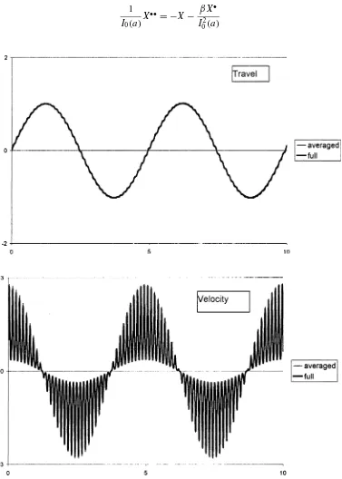
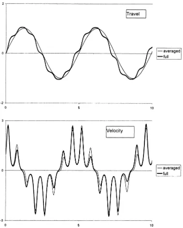
A comparison of the analytical solution with a numerical one illustrates the last statement. It can be found in
figures 1 and 2 for two different values of big parameter (ω=50, figure 1;ω=10, figure 2). In both cases the
calculations were done for the following parameters:
β=0, a=1, ⇒I0(1)≈1,266.
In the first case there is no visible difference between two predictions. For smaller values ofωthe trajectories diverge already at early times.
In figure 1 we can see that the oscillations period is decreased from 2πfor the unperturbed system (a=0) up to 2π/I0(1)≈4,963. One can also see that the solution forxcontains almost only the slow component and the
solution forx•is a superposition of a slow component and of big fast oscillations with slow variable amplitude.
Acknowledgements
The author wishes to thank I.I. Blekhman (Institute of Mechanical Engineering Problems of the Russian Academy of Sciences, St. Petersburg) and R. Fischer (LuK GS GmbH, Buehl, Germany) for their support.
References
Blekhman I.I., 1988. Synchronisation in Science and Technology. ASME Press, New York. Blekhman I.I., 1994. Vibration Mechanics. Nauka, Moscow (in Russian).
Bogoliubov N.N., Mitropolskii Y.A., 1974. Asymptotic Methods in Non-linear Oscillation Theory. Nauka, Moscow (in Russian). Kapitsa P.L., 1951. Dynamic stability of a pendulum with oscillating suspension point. J. Exp. Theor. Phys. 21, 5.
Kapitsa P.L., 1954. Pendulum with vibrating suspension. Achieve. Phys. Sci. 44, 1.
Krylov N.M., Bogoliubov N.N., 1957. Introduction to Non-linear Mechanics. Princeton Univ. Press, Princeton, USA. Nayfeh A.H., 1973. Perturbation Methods. Wiley Interscience, New York.
Nayfeh A.H., Mook D.T., 1979. Non-linear Oscillation. Wiley, New York.
Nayfeh S.A., Nayfeh A.H., 1995. The response of nonlinear systems to modulated high frequency input. Nonlinear Dyn. 7, 310–315. Poincaré H., 1957. Les méthodes nouvelles de mèchanique céleste (3 vol.). Dover, New York.