T H E J O U R N A L O F H U M A N R E S O U R C E S • 45 • 4
Learning
Brian A. Jacob
Lars Lefgren
David P. Sims
A B S T R A C T
This paper constructs a statistical model of learning that suggests a sys-tematic way of measuring the persistence of treatment effects in education. This method is straightforward to implement, allows for comparisons across educational treatments, and can be related to intuitive benchmarks. We demonstrate the methodology using student-teacher linked administra-tive data for North Carolina to examine the persistence of teacher quality. We find that teacher-induced learning has low persistence, with three-quarters or more fading out within one year. Other measures of teacher quality produce similar or lower persistence estimates.
I. Introduction
Educational interventions are often narrowly targeted and temporary, such as class size reductions in kindergarten or summer school in selected elementary grades. Because of financial, political and logistical constraints, evaluations of such programs often focus exclusively on the short-run impacts of the intervention. Insofar as the treatment effects are immediate and permanent, short-term evaluations will provide a good indication of the long-run impacts of the intervention. However, prior research suggests that the positive effects of educational interventions may
Brian Jacob is the Walter H. Annenberg Professor of Education Policy, Professor of Economics, and Director of the Center on Local, State, and Urban Policy (CLOSUP) at the Gerald R. Ford School of Public Policy, University of Michigan. Lars Lefgren is an associate professor of economics at Brigham Young University. David Sims is an assistant professor of economics at Brigham Young University. The authors thank Henry Tappen for excellent research assistance. They thank John DiNardo, Scott Carrell, and Jesse Rothstein and anonymous reviewers as well as seminar participants at MIT, SOLE, Brigham Young University, the University of California, Davis, and Mathematica Policy Research. Scholars may obtain the data used in this article from the North Carolina Education Research Data Center upon sat-isfying their requirements. For information about that process, the authors may be contacted at bajacob@umich.edu, l-lefgren@byu.edu, and davesims@byu.edu, respectively.
[Submitted February 2009; accepted July 2009]
fade out over time (see the work on Head Start by Currie and Thomas 1995, and others). Failure to accurately account for this fadeout can dramatically change the assessment of a program’s impact and/or its cost effectiveness.
Unfortunately, work on measuring the persistence of educational program impacts has not received much emphasis in the applied microeconomics literature, particu-larly in the area of teacher effectiveness which has been a focus of comparatively detailed attention among researchers and policymakers. Indeed, a number of districts and states are experimenting with ways to advance the use of teacher characteristics, including statistically derived “value-added” measures in the design of hiring, cer-tification, compensation, tenure, and accountability policies. An oft-cited claim is that matching a student with a stream of high value-added teachers (one standard deviation above the average teacher) for five years in a row would be enough to completely eliminate the achievement gap between poor and nonpoor students (Riv-kin, Hanushek, and Kain 2005). This prognosis fails, however, to mention the un-derlying assumption of perfectly persistent teacher effects—that is, effects with iden-tical long- and short-run magnitudes.
This paper advances the persistence literature by introducing a framework for estimating and comparing the persistence of treatment effects in education across policy options. To begin, we present a simple model of student learning that incor-porates permanent as well as transitory learning gains. Using this model, we dem-onstrate how the parameter of interest—the persistence of a particular measurable education input—can be recovered via instrumental variables as a local average treatment effect (Imbens and Angrist 1994). We illustrate our method by estimating the persistence of teacher-induced learning gains with multiple measures of teacher quality, though the method generalizes to other educational interventions. Using the student-teacher linkages available in administrative data from North Carolina, we construct measures of teacher effectiveness, including observable teacher correlates of student achievement such as experience and credentials (Clotfelter, Ladd, and Vigdor 2007) as well as statistically derived measures of teacher value-added.
Our resulting estimates suggest that teacher-induced variation in both math and reading achievement quickly erodes. Our point estimates indicate a one-year persis-tence of teacher value-added effects near one-fourth for math and one-fifth for read-ing. Furthermore, we find that the estimated persistence of nontest-based measures of teacher effectiveness is, at best, equal to that of value-added measures. These results are robust to a number of specification checks and suggest that depreciation of a similar magnitude applies to different student racial, gender, and socioeconomic groups. Further estimates suggest that only about one-sixth of the original student gains from a high value-added teacher persist over two years. We further discuss what these estimates can tell us about the relative importance of three fadeout mech-anisms: forgetting, compensatory investment, and future learning rates.
In general, our evidence suggests that even consistent estimates of single-period teacher quality effects drastically overstate the relevant long-run increase in student knowledge. Our results highlight the potential importance of incorporating accurate persistence measures in educational policy evaluation and suggest a comparative framework for implementation.
nonrandom assignment of teachers. However, we are still concerned about the po-tential effects of this bias on our estimates, and we discuss this issue in detail below. We believe that at a minimum our estimates still present a usefulupper bound to the true persistence of teacher effects on student achievement.
The remainder of the paper proceeds as follows. Section II introduces the statis-tical model of student learning, Section III discusses the motivation for examining the persistence of teacher quality, Section IV outlines the data, Section V presents the results, and Section VI contains a short discussion of the paper’s conclusions.
II. A Statistical Model
This section outlines a model of student learning that incorporates permanent as well as transitory learning gains. Our goal is to explicitly illustrate how learning in one period is related to knowledge in subsequent periods. Using this model, we demonstrate how the parameter of interest, the persistence of a par-ticular measurable education input, can be recovered via instrumental variables as a particular local average treatment effect (Imbens and Angrist 1994). We initially motivate this strategy in the context of teacher quality, but then generalize the model to consider other educational interventions.
A. Base Model
In order to control for past student experiences, education researchers often employ empirical strategies that regress (mean zero measures of) current achievement on lagged achievement, namely
Y⳱Y Ⳮε,
(1) t tⳮ1 t
with the common result that the OLS estimate of is less than one. This result is typically given one of two interpretations: Either the lagged achievement score is measured with error due to factors such as guessing, test conditions, or variation in the set of tested concepts, or the coefficient represents the constant depreciation of knowledge over time.
In order to explore the persistence of knowledge, it is useful to specify the learning process underlying these test scores. To begin, suppose that true knowledge in any period is a linear combination of what we describe as “long-term” and “short-term” knowledge, which we label with the subscriptslands. With atsubscript to identify time period, this leads to the following representation:
Y⳱y Ⳮy . (2) t l,t s,t
As the name suggests, long-term knowledge remains with an individual for mul-tiple periods, but is allowed to decay over time. Specifically, we assume that it evolves according to the following process:
where␦ indicates the rate of decay and is assumed to be less than one in order to make y stationary.1 The second term, , represents a teacher’s contribution to
l l,t
long-term knowledge in periodt. The final term,l,t, represents idiosyncratic factors affecting long-term knowledge.
In contrast, short-term knowledge reflects skills and information a student has in one period that decays entirely by the next period.2 Short-run knowledge evolves according to the following process:
y ⳱ Ⳮ , (4) s,t s,t s,t
which mirrors Equation 3 above when ␦, the persistence of long-term knowledge, is zero. Here, the terms,trepresents a teacher’s contribution to the stock of short-term knowledge and s,tcaptures other factors that affect short-term performance.
The same factors that affect the stock of long-term knowledge also could impact the amount of short-term knowledge. For example, a teacher may help students to internalize some concepts, while only briefly presenting others immediately prior to an exam. The former concepts likely form part of long-term knowledge while the latter would be quickly forgotten. Thus it is likely that a given teacher affects both long- and short-term knowledge, though perhaps to different degrees.
It is worth noting that variation in knowledge due to measurement error is ob-servationally equivalent to variation due to the presence of short-run (perfectly de-preciable) knowledge in this model, even though these may reflect different under-lying mechanisms. For example, both a teacher cheating on behalf of students and a teacher who effectively helps students internalize a concept that is tested in only a single year would appear to increase short-term as opposed to long-term knowl-edge. Similarly, a student always forgetting material of a particular nature would appear as short-term knowledge.3 Consequently, our persistence estimates do not
directly distinguish between short-run knowledge that is a consequence of limitations in the ability to measure achievement and short-run knowledge that would have real social value if the student retained it.
In most empirical contexts, the researcher only observes the total of long- and short-run knowledge, Yt⳱yl,tⳭys,t, as is the case when one can only observe a single test score. For simplicity we initially assume thatl,t,l,t,s,t, and s,tare independently and identically distributed, although we will relax this assumption later.4It is then straightforward to show that when considering this composite test
score,Yt, in the typical “value-added” regression model given by Equation 1, the OLS estimate of converges to:
1. This assumption can be relaxed if we restrict our attention to time-series processes of finite duration. In such a case, the variance ofyl,twould tend to increase over time.
2. The same piece of information may be included as a function of either long-term or short-term knowl-edge. For example, a math algorithm used repeatedly over the course of a school year may enter long-term knowledge. Conversely, the same math algorithm, briefly shown immediately prior to the adminis-tration of an exam, could be considered short-term knowledge.
3. This presupposes that understanding the concept does not facilitate the learning of a more advanced concept which is subsequently tested.
2 2 2 yl lⳭl
ˆ
plim
(
)
⳱␦ ⳱␦ .(5) OLS 2Ⳮ2
(
1ⳮ␦)(
2Ⳮ2)
Ⳮ2Ⳮ2 yl ys s s l lThus, OLS identifies the persistence of long-run knowledge multiplied by the frac-tion of variance in total knowledge attributable to long-run knowledge. In other words, one might say that the OLS coefficient measures the average persistence of observed knowledge. The formula above also illustrates the standard attenuation bias result if we reinterpret short-term knowledge as measurement error.
This model allows us to leverage different identification strategies to recover al-ternative parameters of the data generating process. Suppose, for example, that we estimate Equation 3 using instrumental variables with a first-stage relationship given by:
Y ⳱Y Ⳮ ,
(6) tⳮ1 tⳮ2 t
where lagged achievement is regressed on twice-lagged achievement. We will refer to the estimate of from this identification strategy asˆLR, where the subscript is an abbreviation for long-run. It is again straightforward to show that this estimate converges to:
ˆ plim
(
)
⳱␦,(7) LR
which is the persistence of long-run knowledge. Our estimates suggest that this persistence is close to one.
Now consider what happens if we instrument lagged knowledge,Ytⳮ1, with the lagged teacher’s contribution (value-added) to total lagged knowledge. The first stage is given by:
Y ⳱H Ⳮ,
(8) tⳮ1 tⳮ1 t
where the teacher’s total contribution to lagged knowledge is a combination of her contribution to long- and short-run lagged knowledge,H ⳱ Ⳮ . In this
tⳮ1 l,tⳮ1 s,tⳮ1
case, the second-stage estimate, which we refer to asˆVAconverges to:
2 l
ˆ
plim
(
)
⳱␦ .(9) VA 2Ⳮ2
l s
factor or intervention.5Consequently, the estimated persistence of achievement gains
can vary depending on the chosen instrument, as each identifies a different local average treatment effect. In our example,ˆVAmeasures the persistence in test scores due to variation in teacher value-added in isolation from other sources of test score variation whileˆLRmeasures the persistence of long-run knowledge, that is, achieve-ment differences due to prior knowledge.
This suggests a straightforward generalization: to identify the coefficient on lagged test score using an instrumental variables strategy, one can use any factor that is orthogonal toεtas an instrument foryitⳮ1in identifying . Thus, for anyeducational intervention for which assignment is uncorrelated to the residual, one can recover the persistence of treatment-induced learning gains by instrumenting lagged perfor-mance with lagged treatment assignment. Within the framework above, suppose that
and , where and reflect the treatment’s impact on
lt⳱␥ltreatt st⳱␥streatt ␥l ␥s
long- and short-term knowledge respectively.6 In this case, instrumenting lagged
observed knowledge with lagged treatment assignment yields an estimator which converges to the following:
␥l
ˆ
plim
(
)
⳱␦ .(10) TREAT
␥lⳭ␥s
The estimator reflects the persistence of long-term knowledge multiplied by the fraction of the treatment-related test score increase attributable to gains in long-term knowledge.
A standard approach to estimating the persistence of treatment effects is to simply compare the ratio of coefficients from separate treatment effect regressions at dif-ferent points in the future. For example, one might estimate the impact of a child’s current fifth grade teacher on her contemporaneous fifth grade test scores, and then in a second regression estimate the impact of the child’s former (in this case fourth grade) teacher on her fifth grade test scores. The ratio of the teacher coefficient from the second regression to the analogous coefficient in the first regression provides a measure of the one-year persistence of the teacher effect.
While this approach does provide a measure of persistence, our approach has a number of advantages over the informal examination of coefficient ratios. First, it provides a straightforward way to both compute estimates and conduct inference on persistence measures through standard t- and F-tests.7 Second, the estimates of and serve as intuitive benchmarks that allow an understanding of the
ˆ ˆ
LR OLS
relative importance of teacher value-added as opposed to test scaling effects. They allow us to examine the persistence of policy-induced learning shocks relative to the respective effects of transformative learning and a “business as usual” index of educational persistence. Finally, the methodology can be applied to compare
persis-5. Given a different data generating process the structural interpretation ofˆOLSandˆLRmay change but they will still retain the LATE interpretation as the persistence arising from all sources of achievement variation and long-run differences in achievement respectively.
6. While treat could be a binary assignment status indicator, it could also specify a continuous policy variable such as educational spending or class size.
tence among policy treatments including those that may be continuous or on different scales such as hours of tutoring versus number of students in a class.
B. Extensions
Returning to our examination of the persistence of teacher-induced learning gains, we relax some assumptions regarding our data generating process to highlight al-ternative interpretations of our estimates as well as threats to identification. First, consider a setting in which a teacher’s impacts on long- and short-term knowledge are not independent. In that caseˆVAconverges to:
2
While␦maintains the same interpretation, the remainder of the expression is equiv-alent to the coefficient from a bivariate regression of on H. In other words, it
l
captures the rate at which a teacher’s impact on long-term knowledge increases with the teacher’s contribution to total measured knowledge.
Another interesting consequence of relaxing this independence assumption is that
need not be positive. In fact, if 2 will be negative. This
VA cov
(
l,s)
⬍ⳮl,VAcan only be true if 2 2. This would happen if observed value-added captured
⬍ l s
primarily a teacher’s ability to induce short-term gains in achievement and this is negatively correlated to a teacher’s ability to raise long-term achievement. Although this is an extreme case, it is clearly possible and serves to highlight the importance of understanding the long-run impacts of teacher value-added.8,9
Although relaxing the independence assumption does not violate any of the re-strictions for satisfactory instrumental variables identification,VAcan no longer be interpreted as a true persistence measure. Instead, it identifies the extent to which teacher-induced achievement gains predict subsequent achievement.
However, there are some threats to identification that we initially ruled out by assumption. For example, suppose that cov
(
,)
⬆0, as would occur if schooll,t l,t
administrators systematically allocate children with unobserved high learning to the best teachers. The opposite could occur if principals assign the best teachers to children with the lowest learning potential. In either case, the effect on our estimate depends on the sign of the covariance, since:
2
8. The teacher cheating in Chicago identified by Jacob and Levitt (2003) led to large observed performance increases, but was correlated to poor actual performance in the classroom. Also, Carrell and West (2008) show that short run value-added among Air Force Academy Faculty is negatively correlated to long-run value-added.
9. In general, theplim(ˆ )is bounded between␦ l when the correlation between short and long VA
lⳮs run value-added isⳮ1 and␦ l when it is 1.
If students with the best idiosyncratic learning shocks are matched with high-quality teachers, the estimated degree of persistence will be biased upward. In the context of standard instrumental variables estimation, lagged teacher quality fails to satisfy the necessary exclusion restriction because it affects later achievement through its correlation with unobserved educational inputs. To address this concern, we show the sensitivity of our persistence measures to the inclusion of student-level covariates and contemporaneous classroom fixed effects in the second-stage regression, which would be captured in thelterm. Indeed, the inclusion of student covariates reduces the estimated persistence measure, which suggests that such a simple positive selec-tion story is the most likely and our persistence measures are overestimates of true persistence. On the other hand, Rothstein (2010) argues that the matching of teachers to students is based in part on transitory gains on the part of students in the previous year. This story might suggest that we underestimate persistence, as the students with the largest learning gains in the prior year are assigned the least effective teachers in the current year.
Another potential problem is that teacher value-added may be correlated over time for an individual student. If this correlation is positive, perhaps because motivated parents request effective teachers every period, the measure of persistence will be biased upward. We explore this prediction by testing how the coefficient estimates change when we omit our controls for student level characteristics. In our case the inclusion of successive levels of control variables monotonically reduces our persis-tence estimate, as the positive sorting story would predict.
III. Background
A. Teacher Quality and Value-Added Measures
Lefgren 2008) in differentiating among certain regions of the teacher quality distri-bution, the increasing use of value-added measures seems likely wherever the data requirements can be met.
At the same time, a number of recent studies (Andrabi et al. 2008; McCaffrey et al. 2004; Rothstein 2010; Todd and Wolpin 2003, 2006) highlight the strong as-sumptions of the most commonly used value-added models, suggesting that they are unlikely to hold in observational settings. The most important of these assumptions in our present context is that the assignment of students to teachers is random. Indeed given random assignment of students to teachers, many of the uncertainties regarding precise functional form become less important. If students are not assigned randomly to teachers, positive outcomes attributed to a given teacher may simply result from teaching better students. In particular, Rothstein (2010) raises disturbing questions about the validity of current teacher value-added measurements, showing that the
currentperformance of students can be predicted by the value-added of theirfuture
teachers.
However, in a recent attempt to validate observationally derived value-added methods with experimental data, Kane and Staiger (2008) were unable to reject the hypothesis that the observational estimates were unbiased predictions of student achievement in many specifications. Indeed, one common result seems to be that models that control for lagged test scores, such as our model, tend to perform better against these criticisms than gains models.
B. Prior Literature
As Todd and Wolpin (2003) note, much of the early research on teacher value-added fails to explicitly consider the implications of imperfect persistence. For example, the Rivkin, Hanushek, and Kain (2005) scenario of “five good teachers” assumes perfect persistence of student gains due to teacher quality. As a result, these studies imply that variation in test score increases due to policy changes will have long-run consequences equivalent to those of test score increases that come from increased parental investment or innate student ability.
The first paper to explicitly consider the issue of persistence in the effect of teachers on student achievement was a study by McCaffery et al. (2004). Although their primary objective is to test the stability of teacher value-added models to vari-ous modeling assumptions, they also provide parameter estimates from a general model that explicitly considers the one- and two-year persistence of teacher effects on math scores for a sample of 678 third through fifth graders from five schools in a large school district. Their results suggest one-year persistence of 0.2 to 0.3 and two-year persistence of 0.1. However, due to the small sample the standard errors on each of these parameter estimates was approximately 0.2.
More recently, a contemporary group of teacher value-added studies have emerged that recognize the importance of persistence. For example, Kane and Staiger (2008) use a combination of experimental and nonexperimental data from Los Angeles to examine the degree of bias present in value-added estimates due to nonrandom assignment of students to teachers. They note that coefficient ratios taken from their results imply a one-year math persistence of one-half and a language arts persistence of 60–70 percent. When they expand their sample to include a more representative group of students and control for additional student characteristics, their persistence estimates drop to near one-fourth. Similarly, Rothstein (2010) mentions the impor-tance of measuring fadeout and presents evidence of persistence effects for a par-ticular teacher around 40 percent. Carrell and West (2008) present evidence that more experienced university professors at the Air Force academy induce lower but more persistent variation in student learning.
In summary, while the recent teacher value-added literature has come to recognize the need to account for persistence, it and the broader education production literature still lack a straightforward, systematic way to test hypotheses about persistence and to make cross-program persistence comparisons. Persistence is usually inferred as the informal ratio of coefficients from separate regressions, abstracting from the construction and scaling of the particular exam scores. This seems to be an important omission given previous research suggesting decay rates for educational interven-tions that vary widely across programs; from long-term successes such as the Ten-nessee class size experiment (Nye, Hedges, and Konstantopoulos 1999; Krueger and Whitmore 2001) or the Perry preschool project (Barnett 1985), to programs with no persistent academic effects such as Head Start (Currie and Thomas 1995) or grade retention for sixth graders (Jacob and Lefgren 2004).
C. Interpreting Persistence
Our measure of persistence reflects three different mechanisms. First, students may forget information or lose skills that they acquired as a result of a particular teacher or intervention. Second, students or schools may engage in potentially endogenous subsequent investments, which either mitigate or exacerbate the consequences of assignment to a particular teacher or intervention. Third, our persistence measure depends on how the knowledge learned from a particular teacher influences student learning of new material.
elementary school math and reading, in which there is considerable overlap from year to year, this extreme case seems unlikely. Hence, in our analysis, we believe that persistence will largely reflect the first two mechanisms, forgetfulness and com-pensatory investments.
Changes over time in the statistical properties of a test, such as variance, also may affect the interpretation of a persistence estimate. If observed performance captures neither a cardinal measure of performance nor a uniformly measured rank, it is impossible to arrive at a unique, interpretable estimate of persistence. For example, suppose the test metric functions as an achievement ranking but the variance of the performance metric differs across years. In such cases, the observed persistence measure will reflect both the fadeout of teacher-induced changes in rank as well as the cross-year heteroskedasticity of achievement measures. Whatever the true per-sistence in knowledge, the test scale can be compressed or stretched to produce any desired estimate of fadeout.
This might lead some observers to discount the usefulness of persistence measures in general or reject those estimates they find disagreeable. To us, however, this potential sensitivity of observed persistence to test scale effects underscores the importance of establishing baseline measures of the general persistence of knowledge to which the persistence of teacher-induced knowledge can be compared. In this study, we present two such benchmarks, which allow us to compare the persistence of teacher-induced learning to more familiar sources of variation.
One final concern with interpreting our persistence measures involves the possi-bility of test manipulation. For example, Jacob and Levitt (2003) document a number of cases of teacher cheating, which led to large observed performance increases in one year that did not persist in subsequent years. Similarly, Carrell, and West’s (2008) finding that teacher effects from one year of class can be negatively correlated with future years’ exam scores is likely explained by contrasting just such a short-run strategic focus on the part of some teachers with a forward-looking approach on the part of other instructors. Such behaviors would manifest themselves in low observed persistence that one might ascribe to poor test measurement—that is, one might argue that there was no true learning in such cases in the first place.
IV. Data
A. The Sample
To measure the persistence of teacher-induced learning gains, we use a data set derived from North Carolina school administrative records maintained by the North Carolina Education Research Data Center. The primary data consists of student-year observations for all students in third through sixth grades in the state from 1997– 2004.10During this time period North Carolina required end-of-course standardized
exams for all these students in both reading and mathematics that were closely aligned to the state’s learning standards.
We follow the practice of earlier researchers (Clotfelter, Ladd, and Vigdor 2007) by standardizing the North Carolina scores to reflect standard-deviation units relative to the state average for that grade and year. Thus, our resulting persistence measure captures the degree to which a teacher’s ability to change a student’s rank (measured in standard deviations) in the achievement distribution is manifest in the student’s rank in subsequent years. This relative measure not only allows for comparability of our results with the prior literature, but also captures the effect of a policy on the ranking of a student at some future date such as entry into the labor market. We also show in our robustness checks that our results are robust to the use of scaled scores, which are designed to approximate an absolute measure of learning.
These student-year records can be matched to personnel record data for classroom teachers that contain information on teacher experience, credentials, and certification. We follow the algorithm described in detail in Clotfelter, Ladd, and Vigdor (2007) to match teachers to students.11 This allows an approximately 79 percent match
success rate for a student’s prior year teacher (for whom we wish to calculate per-sistence). Because the most accurate matching of students to teachers is only possible for third through fifth grade students in this data, and because we require one year of lagged test scores as an instrument to capture long-run learning persistence, we calculate value-added over the set of fourth and fifth grade teachers, and measure outcomes for these students in fifth and sixth grades.12Beyond the matching error
rate, the measurement of teacher experience may be a concern as it is calculated as the years for which the teacher is given credit on the salary schedule, (whether those years were in North Carolina or not) a potentially noisy measure of true experience. Table 1 reports summary statistics including the basic demographic controls for student race, ethnicity, free lunch, and special education status available in the data. While the North Carolina sample is close to the national average in free lunch eligibility (44 percent compared to 42 percent nationally), it actually has smaller than average minority enrollments, comprised mainly of African-American students, and has only a small percentage of nonnative English speakers. About one-eighth of students in North Carolina have a novice teacher (a teacher in his or her first two years of teaching), and a relatively large proportion of teachers, almost 10 percent, receive national board certification at some point in the sample period. This latter figure is likely driven by the 12 percent salary premium attached to this certification.
B. Estimating Teacher Value-Added
To measure the persistence of teacher-induced learning gains we must first estimate teacher value-added. Consider a learning equation of the following form.
test ⳱test ⳭX CⳭⳭ Ⳮε ,
(13) ijt itⳮ1 it j jt ijt
11. The teachers identified in the student test file are those that proctored the exam, not necessarily those that taught the class. The authors describe the three-tiered system of matching students to actual teachers. The first assigns the proctor as the teacher if the proctor taught the correct grade and subject that year. They also look at the composition of the test taking students and compare it with the composition of students in classes from the teacher file to find matches.
Table 1
Summary Statistics
Variable North Carolina
Normalized reading score 0.000
(1.000)
Normalized math score 0.000
(1.000)
Student fraction male 0.508
(0.500)
Student fraction free lunch 0.440
(0.496)
Student fraction White 0.625
(0.484)
Student fraction Black 0.296
(0.457)
Student fraction Hispanic 0.035
(0.184)
Student fraction special education 0.110
(0.312)
Student fraction limited English 0.016
(0.124)
Student age 11.798
(0.721)
Student has novice teacher 0.123
(0.328)
Student has board certified teacher 0.098
(0.297)
Fifth grade 0.499
(0.500)
Sixth grade 0.501
(0.500)
wheretestitis a test score for individualiin periodt,Xitis a set of potentially time varying covariates,jcaptures teacher value-added,jtreflects period specific class-room factors that affect performance (for example, a test administered on a hot day or unusually good match quality between the teacher and students), andεitis a mean zero residual.
We have two concerns about our estimates of teacher value-added. The first, discussed earlier, is that the value-added measures may be inconsistent due to the nonrandom assignment of students to teachers. The second is that the imprecision of our estimates may affect the implementation of our strategy. Standard fixed effects estimation of teacher value-added relies on test score variation due to classroom-specific learning shocks,jt, as well as student specific residuals,εijt. Because of this, the estimation error in teacher value-added will be correlated to contempora-neous student achievement and fail to satisfy the necessary exclusion restrictions for consistent instrumental variables identification.
To avoid this problem, we estimate the value-added of a student’s teacher that does not incorporate information from that student’s cohort. Specifically, for each year by grade set of student observations we estimate a separate regression of the form:
test ⳱test ⳭX CⳭ Ⳮ ,
(14) ijy iyⳮ1 iy jy ijy
where indexing of student and teacher remains as above andynow indexes year.X
is a vector of control variables including the student’s age, race, gender, free-lunch eligibility, special education placement, and limited English proficiency status. Then for each student iwith teacherjin yeartwe compute an average of his teacher’s value-added measures across all years in which that student wasnotin the teacher’s classroom, but in the same school.
⳱
(15) ijt
兺
jyy⬆t
Consider, for example, a teacher who taught in school A from 1995–99 and in school B from 2000–2003. For a student in the teacher’s class in 1996, we use a value-added measure that incorporates data from that teacher’s classes in 1995 and 1997– 99. For a student in the teacher’s class in 2000, we use a value-added measure incorporating data from 2001–2003.13 The estimation error of the resulting
value-added measures will be uncorrelated to unobserved classroom-specific determinants of the reference student’s achievement. As discussed later, the results of our
jt
estimation are robust to various specifications of the initial value-added equation. Our second-stage equation for estimating the persistence of teacher value-added then becomes:
test ⳱ test ⳭX CⳭ Ⳮ Ⳮ␥ Ⳮε
(16) ijtⳭ1 VA it itⳭ1 jtⳭ1 tⳭ1 g ijtⳭ1
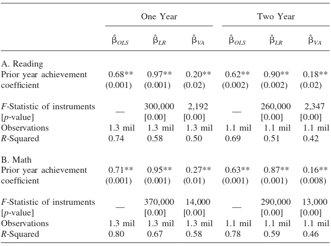
Table 2
Estimates of the Persistence of Achievement
One Year Two Year
F-Statistic of instruments 300,000 2,192 260,000 2,347 [p-value] — [0.00] [0.00] — [0.00] [0.00] Observations 1.3 mil 1.3 mil 1.3 mil 1.1 mil 1.1 mil 1.1 mil R-Squared 0.74 0.58 0.50 0.69 0.51 0.42
B. Math
F-Statistic of instruments 370,000 14,000 290,000 13,000 [p-value] — [0.00] [0.00] — [0.00] [0.00] Observations 1.3 mil 1.3 mil 1.3 mil 1.1 mil 1.1 mil 1.1 mil R-Squared 0.80 0.67 0.58 0.78 0.59 0.46
Notes: Reported standard errors in parentheses correct for clustering at the classroom level. ** indicates 5 percent significance.
whereijtfrom Equation 15 serve as the excluded instruments in the first stage. The specification includes the above mentioned student level controls as well as grade, year, and contemporary classroom (teacher) fixed effects. In our second stage, we include classroom fixed effects (which subsume school fixed effects). Thus, our estimation relies exclusively on variation in teacher quality within a school.
V. Results
the general result that around two-thirds of the variation in student level test scores is likely to persist after a year is a benchmark figure confirmed by other studies.14
Instrumental variables estimates of long-run learning persistence, ˆLR, use twice lagged test scores and an indicator for a missing twice lagged score as the excluded instruments. The estimates suggest that variation in test scores caused by prior (long-run) learning is almost completely persistent after one year, with estimated values a little below one in both cases.15
When compared against these baselines, the achievement differences due to a high value-added teacher, ˆVA, are more ephemeral. The point estimates suggest that between 0.20–0.27 of the initial test score variation is preserved after the first year. While we statistically reject the hypothesis of zero persistence, the effects are sig-nificantly lower than either benchmark. For the instrumental variables estimates, the table also reports theF-statistic of the instruments used in the first stage. In all cases, the instruments have sufficient power to make a weak instruments problem un-likely.16
While the simple model presented in Section II assumes a specific decay process for knowledge, we recognize that this is unlikely to be a complete description of the depreciation of learning. Thus, the final three columns of Table 2 expand the analysis to consider the persistence of achievement after two years. The estimation strategy is analogous to the previous specification, except that the coefficient of interest comes from the second lag of student test scores. All instruments are also lagged an additional year. In all cases, the two-year persistence measures are smaller than the one-year persistence measures. In reading, persistence measures in test score variation due to teacher value-added drop only two percentage points from their one-year levels while math scores appear to lose a third of their one-one-year persistence.
It may seem slightly surprising that after the observed erosion of the majority of value-added variation in a single year, students in the next year lose a much smaller fraction. This suggests that our data-generating model may be a good approximation to the actual learning environment in that much of the achievement gain maintained beyond the first year is permanent. Alternatively, it may be that even conditional upon our covariates, our measure of persistence still reflects unobserved heteroge-neity in the permanent, unobserved ability of the student. In any event, the large majority of the overall gain commonly attributed to value-added is a temporary one-period increase.
These results are largely consistent with the published evidence on persistence presented by McCaffery et al. (2004) and Lockwood et al. (2007). Both find one-and two-year persistence measures between 0.1 one-and 0.3. However, our estimates are smaller than those of contemporary papers by Rothstein (2010) and Kane and Staiger (2008), which both suggest one-year persistence rates of 0.4 or greater. As mentioned earlier, different persistence estimates within this band may reflect a different weight-ing of fadeout mechanisms as well as different scalweight-ing issues across outcome mea-sures. Thus, perhaps the most important contrast in the Table is the persistence of
14. See, for example, Todd and Wolpin (2006) and Sass (2006).
15. The first stage estimates are very similar to the OLS persistence measures.
Table 3
(2) Controllingonlyfor grade, school, and year in second stage
(3) Omitting yeartclassroom fixed effects from baseline
(6) Top third of teacher quality compared to middle third
(7) Bottom third of teacher quality compared to middle
Notes: Reported standard errors in parentheses correct for clustering at the classroom level.
** indicates 5 percent significance. Though not reported, estimation results for benchmarkˆLRare quite consistent across the table’s specifications with estimates on always in the 0.95–0.99 range for reading scores and the 0.93–0.97 range for math scores.
teacher value-added in relation to the benchmarks. If we think of ˆLR as transfor-mative learning, we find that teacher value-added is only one-fourth to one-fifth as persistent, as well as less than half as persistent as the average inputs mark repre-sented by ˆOLS.
value-added is the possibility of nonrandom assignment of students to teachers, both con-temporaneously, and in prior years. Although we attempt to deal with this possibility with a value-added model and the inclusion of student characteristics in the regres-sion, it is still possible that we fail to account for systematic variation in the assign-ment of students to teachers. The first three rows of the table show that relaxing our control strategy results in increases to the estimated persistence. For example, omit-ting classroom effects (Row 3) from the regression leads to significant increases in the estimated persistence, while dropping all other student controls leads the coef-ficients to increase by a third or more (Row 2). This demonstration of positive selection on observables is consistent with our belief that ourˆVAestimate reflects an upper bound in the face of likely positive selection on unobservables. Thus the most likely identification failure suggests an even lower persistence than we find in Table 2.
We have estimated our model using a representation of teacher value-added that controls for lagged student achievement as it may avoid many of the problems associated with the value-added models denominated in terms of test score gains. However, the gains formulation remains popular and Rows 4–5 show the robustness of our estimates to the use of a gains model in calculating our teacher value-added measures. In the case of math, the switch to a gains specification of value-added has no meaningful effect and in the case of reading it serves only to decrease the estimated persistence by 25–50 percent.
To this point, we have only been measuring the average persistence of teacher-induced test score variation without considering whether the effects are symmetric with respect to the sign of the shocks. Given that persistence measures might be driven by students at the bottom catching up due to nonrandom school interventions, it seems important to examine the symmetry of the persistence effects. In other words, we wish to see whether the test score consequences of having an uncom-monly bad teacher are more or less lasting than the benefits of having an excep-tionally good teacher. Rows 6–7 of Table 3 show the comparison between effects at the top and bottom of the respective distributions. In all cases, we are unable to reject equal persistence values for both sides of the teacher distribution, though the point estimates are larger for the lower tail.17
In the final two rows of Table 3, we examine the sensitivity of our estimates to the scaling of the exam. In Row 8, we measure test performance as the achieved percentile within state*year. In Row 9, we use the scale score measures, which are commonly treated as if they possessed a cardinal interpretation. Despite ex-ante concerns that the results may differ, they are surprisingly similar to our baseline suggesting that our finding is not sensitive to the choice among a variety of sensible
academic performance measures. Furthermore, examination of theˆLR benchmark for scaled scores finds an estimate of 0.96 for both reading and math, quite close to the standardized benchmark.
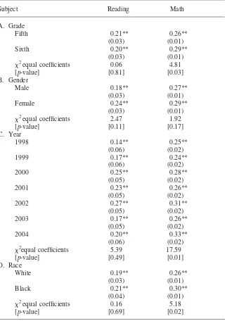
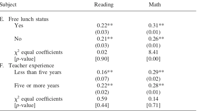
Since conclusions concerning the persistence of teacher quality might depend on the heterogeneity of persistence across different groups of students, Table 4 shows how persistence estimates differ across measurable student characteristics as well as year, grade, and teacher experience. For reading scores, there is no evidence of statistically significant heterogeneity of persistence effects across grade, gender, race, test year or free lunch status. For math scores, on the other hand, there appears to be statistically significant differences in persistence across all the above groups ex-cept gender. However, the difference in actual magnitudes is small, with a range between 0.03–0.05 for all categories except test year. This uniformity across student groups suggests our measure may be capturing a common effect. The final panel of the table suggests that the persistence of teacher effects is not meaningfully different for experienced versus inexperienced teachers.
For the specifications reported in Tables 3 and 4 it is also possible to estimate our benchmarkˆLR. The results are quite consistent across specifications with es-timates always in the 0.95–0.99 range for reading scores and the 0.93–0.97 range for math scores. Given this small range we have chosen not to report all these values in the tables. Nevertheless, the benchmark results strengthen our case for comparing the results ofˆVAacross specifications.
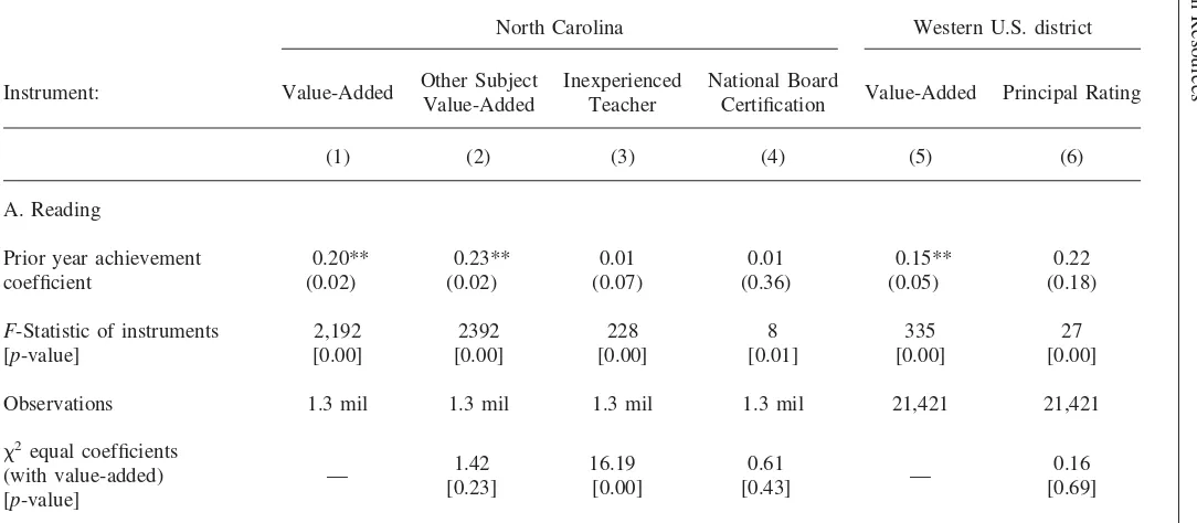
Although these results about the persistence of teacher value-added are important, there is always the possibility that the nature of value-added measures, as a sort of teacher fixed effect on test scores, leaves them particularly vulnerable to measuring strategic teacher manipulations that add little social value, such as the ability to teach to a particular test. One possible way to explore this is to use a teacher’s measure of value-added in the opposite subject (for example, reading value-added as an instrument for the students past math score) as the excluded instrument. The results of this specification are reported in the second column of Table 5. While there is a statistically significant difference between this and the baseline estimates for math, the magnitude of the point estimates are virtually identical. Of course this could mean either that teaching to the test is not an important component of teacher value-added in this setting or that the ability to teach to the test has a high positive correlation across subjects.
Table 4
Heterogeneity of One-Year Depreciation Rates
Subject Reading Math
2equal coefficients 0.06 4.81
[p-value] [0.81] [0.03]
2equal coefficients 2.47 1.92
[p-value] [0.11] [0.17]
2equal coefficients 5.39 17.59
[p-value] [0.49] [0.01]
2equal coefficients 0.16 5.18
[p-value] [0.69] [0.02]
Table 4(continued)
Subject Reading Math
E. Free lunch status
Yes 0.22**
(0.03)
0.31** (0.01)
No 0.21**
(0.03)
0.26** (0.01)
2equal coefficients 0.02 8.41
[p-value] [0.90] [0.00]
F. Teacher experience
Less than five years 0.16**
(0.07)
0.29** (0.02)
Five or more years 0.22**
(0.02)
0.28** (0.01)
2equal coefficients 0.59 0.14
[p-value] [0.44] [0.71]
Notes: Reported standard errors in parentheses correct for clustering at the classroom level. ** indicates 5 percent significance. Though not reported, estimation results for benchmarkˆLRare quite consistent across the table’s specifications with estimates on always in the 0.95–0.99 range for reading scores and the 0.93– 0.97 range for math scores.
final test score of interest) as well as observable student characteristics and school and year fixed effects. The residuals from these regressions serve as our instruments. This is analogous to the process of producing our teacher value-added instruments outlined above.
In both math and reading, the coefficient estimates are significantly lower than the corresponding value-added estimates, suggesting that teacher experience shocks generateless persistent effects than value-added shocks. In fact, it is impossible to reject a zero persistence outcome for the effect of teacher inexperience on reading scores.
The fourth column looks at the persistence of test score shocks generated by having a teacher with National Board Certification (NBC). More specifically, we define a teacher as having NBC if he or she ever appears as certified in our data. For this reason, our measure is capturing both any teacher characteristics associated with the propensity to apply for and receive certification as well as any “effects” of the certification process itself.18Following the logic described above, as our
instru-ment we use residuals from a regression of NBC status on lagged student achieve-ment and student demographics rather than the raw NBC indicator. For math, the persistence of having a NBC teacher is roughly equivalent to having a teacher with a value-added measure one standard deviation higher than average. For reading, the
The
Journal
of
Human
Resources
Table 5
Comparing Value-Added Persistence with Other Teacher Policies
North Carolina Western U.S. district
Instrument: Value-Added Other Subject Value-Added
Inexperienced Teacher
National Board
Certification Value-Added Principal Rating
(1) (2) (3) (4) (5) (6)
A. Reading
Prior year achievement coefficient
0.20** (0.02)
0.23** (0.02)
0.01 (0.07)
0.01 (0.36)
0.15** (0.05)
0.22 (0.18)
F-Statistic of instruments [p-value]
2,192 [0.00]
2392 [0.00]
228 [0.00]
8 [0.01]
335 [0.00]
27 [0.00]
Observations 1.3 mil 1.3 mil 1.3 mil 1.3 mil 21,421 21,421
2equal coefficients
(with value-added) [p-value]
— 1.42 [0.23]
16.19 [0.00]
0.61
[0.43] —
Jacob,
Lefgren,
and
Sims
937
Prior year achievement coefficient
0.27** (0.01)
0.25** (0.01)
0.10** (0.04)
0.22** (0.08)
0.17** (0.05)
0.15 (0.12)
F-Statistic of instruments [p-value]
14,000 [0.00]
4768 [0.00]
440 [0.00]
110 [0.00]
325 [0.00]
44 [0.00]
Observations 1.3 mil 1.3 mil 1.3 mil 1.3 mil 21,421 21,421
2equal coefficients
(with value-added) [p-value]
— 8.59 [0.00]
22.29 [0.00]
0.55
[0.46] —
0.06 [0.81]
point estimate of the NBC persistence is nearly zero, although the estimate is quite imprecise.
As a further specification check, we perform a similar analysis of teacher value-added and another teacher quality measure on a separate longitudinal data set that matches students to teachers from 1998 to 2004 in an anonymous mid-sized Western school district. This allows us to check whether our persistence estimates might be sensitive to the particular set of institutions or tests given in North Carolina. Using this data in standard deviation units, we constructed analogous measures of teacher value-added and examined the persistence of test scores due to the resulting variation in teacher value-added.
The presentation of results in Columns 5–6 shows the estimated persistence of teacher value-added in this district is even lower than in North Carolina. The point estimates suggest a one-year persistence of 0.15 for reading and 0.17 for math.19In both cases, we reject the hypothesis of zero persistence. This school district also has an alternative available measure of teacher quality, a numeric principal evaluation of the teacher’s performance. The persistence estimates in Column 6 suggest that the components of teacher quality captured in principal evaluations have similar persistence to those captured by value-added measures, although these estimates are also quite imprecise. These results are important because they suggest that the low measured persistence of teacher value-added is not a peculiarity of North Carolina schools or one specific test metric.
While our preferred estimation strategy has a number of advantages relative to other approaches, we should be able to recover similar persistence measures using a reduced form strategy. One potential difficulty is that we do not observe actual teacher quality but rather a noisy proxy leading a regression of student achievement on raw value-added measures to exhibit substantial attenuation bias.20To overcome
this problem, we can construct empirical Bayes measures of teacher quality, which “shrink” a teacher’s estimated value-added to the grand mean of teacher quality according to the precision of the estimate. The goal is to estimate the expected teacher quality conditional upon the observed noisy signal.
Morris (1983) describes a method for implementing parametric empirical Bayes (EB) estimators.21Briefly, to obtain EB estimates of teacher quality, we multiply
each raw value-added measure by its statistical reliability. This shrinks each estimate toward zero, which is the mean of teacher quality by construction.22For our
reli-19. The benchmark estimates show an estimated persistence of student achievement captured by OLS at 0.58 on both tests and an estimated persistence of long-run knowledge of 1.07 for reading and 1.08 for math. If the slightly elevated long-run estimates are an estimate of scale, the western districts teacher value-added fadeout looks even steeper relative to North Carolina.
20. This is not a problem in the context of our instrumental variables strategy, which is robust to mea-surement error in teacher quality as long as it is uncorrelated to the second-stage residual.
21. Education researchers often use Hierarchical Linear Modeling (HLM) to obtain Bayesian estimates of teacher quality. Kane and Staiger (2008) employ an approach similar to our own and determine that the correlation between their EB estimates of teacher quality and those obtained by HLM have a correlation that exceeds .99.
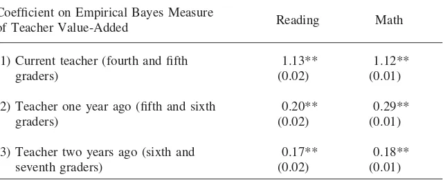
Table 6
Reduced Form Impact of Current and Lagged Teacher Value-Added on Student Achievement
Coefficient on Empirical Bayes Measure
of Teacher Value-Added Reading Math
(1) Current teacher (fourth and fifth graders)
1.13** (0.02)
1.12** (0.01)
(2) Teacher one year ago (fifth and sixth graders)
0.20** (0.02)
0.29** (0.01)
(3) Teacher two years ago (sixth and seventh graders)
0.17** (0.02)
0.18** (0.01)
Notes: The reported coefficients are obtained from six separate regressions. The construction of the em-pirical Bayes measures of teacher value-added is described in the text. In addition to the same controls used in the IV specifications, we control for prior year reading and math achievement in Row 1, twice lagged achievement in Row 2, and thrice lagged achievement in Row 3. In Rows 2–3, we also control for current classroom fixed effects. In Row 1, the classroom fixed effect is collinear with current teacher value-added so we control for control for classroom composition with the average prior year reading and math scores. Reported standard errors in parentheses correct for clustering at the classroom level. ** indicates 5 percent significance.
ability calculation, we obtain an estimate of the true variance by calculating the covariance between measures of teacher value-added estimated for the same teacher in different periods and calculate the estimation error by subtracting it from the variance of teacher value-added estimates calculated with a single year of data.
To identify the reduced form impact of current teacher quality on student achieve-ment, we estimate the following regression for fourth and fifth grade students:
EB
ˆ
test ⳱␣ Ⳮtest ⳭX CⳭε .
(17) ijt j itⳮ1 it ijt
Our covariates include a student’s own lagged reading and math achievement along with the demographic controls used in our baseline IV specifications. The inclusion of classroom fixed effects is not possible as it would be collinear with the current teacher’s value-added score. Thus we control for classroom composition by includ-ing classroom average lagged readinclud-ing and math performance. We use standard errors that are robust to clustering within the classroom. The coefficients from this regres-sion are found in Row 1 of Table 6. We see that the coefficient on the EB measure of reading and math achievement are approximately 1.1. With the EB approach, we would have expected the coefficient to be very close to one. The fact that it exceeds this value may reflect some nonrandom assignment of high-ability children to teach-ers with high observed value-added.
include current classroom fixed effects that subsume the average classroom perfor-mance measures and control more effectively for classroom composition and selec-tion. The reduced form estimates of the impact of lagged teacher quality are 0.20 for reading and 0.29 for math. These are virtually identical to our IV persistence measures. If we divide them by the initial period effects, they are slightly lower though substantively the same.
Row 3 shows the impact of twice lagged teacher value-added. Relative to the lagged specification, the only differences are that we examine students in the seventh and eighth grades and control for thrice lagged achievement. The coefficients on the twice lagged teacher value-added measures are 0.17 for reading and 0.18 for math, again very consistent with our IV persistence estimates.
VI. Conclusions
This paper develops a statistical framework to empirically assess and compare the persistence of treatment effects in education. We present a model of student learning that incorporates permanent as well as transitory learning gains, and then demonstrates that an intuitive instrumental variables estimator can recover the persistence parameter.
The primary claim of the recent teacher value-added literature is that teacher quality matters a great deal for student achievement. This claim is based on consis-tent findings of a large dispersion in teachers’ ability to influence contemporary student test scores. While this claim may well be true relative to other policy alter-natives, our results indicate that contemporaneous value-added measures are a poor indicator of long-term added. Indeed, test score variation due to teacher value-added is only about one-fifth as persistent as true long-run knowledge and perhaps one-third as persistent as the overall variation in test scores. Thus when measured against intuitive benchmarks, contemporary teacher value-added measures almost certainly overstate the ability of teachers, even exceptional ones, to influence the ultimate level of student knowledge.
Furthermore, when measured against other potential policy levers that involve teacher quality, value-added induced variations do not have statistically different persistence than those of principal ratings or national board certification measures. We do find, however, that value-added variation in student achievement is signifi-cantly more persistent than the variation generated by inexperienced teachers.
Taken at face value, our results for two-year persistence imply that a policy in-tervention to raise teacher value-added by a standard deviation would produce a long-run effect on student math achievement closer to 0.02 standard deviations than the 0.10 standard deviation increase found in the literature (Aaronson, Barrow, and Sander 2007; Rivkin, Hanushek, and Kain 2005; Rockoff 2004).
Ac-cording to Figlio and Kenney (2007), a merit pay program to move beyond identi-fication to retention might be expected to improve student achievement by 0.05– 0.09 standard deviations. However, the cost of testing and bonuses for such a program becomes significantly harder to justify if the relevant effect size is at most 0.009–0.016 standard deviations when measured just two years later.
As mentioned earlier, our statistical model captures knowledge fadeout stemming from a variety of different sources, ranging from poor measurement of student knowledge to structural elements in the education system that lead to real knowledge depreciation. Although it is impossible in the present context to definitively label one or more explanations as verified, we can make some progress in this area. For example, our results show that the low persistence of teacher quality-induced vari-ation is not due to some flaw in the construction or use of value-added measures, but is common to other methods of measuring teacher quality.
Our results also provide some evidence that the observed fadeout is not due to compensatory teacher assignment. Indeed, measured persistence declines when con-trolling for the current class-room fixed effects suggesting that teacher quality is positively correlated over time. This positive autocorrelation is observed directly when we look at the correlation between the measured value-added of the student’s prior year teacher and the student’s teacher two years ago.
Should the particular explanation for fadeout change how we should think about the policy possibilities of value-added? To examine this, consider under what cir-cumstances exceptional teachers could have widespread and enduring effects in ways that belie our estimates. Three criteria would have to be met: The knowledge that students could obtain from these exceptional teachers would have to be valuable to the true long-run outcomes of interest (such as wages or future happiness), retained by the student, and not tested on future exams. To the degree that all three of these conditions exist, the implications of this analysis should be tempered.
Although it is certainly possible that these conditions are all met, we believe it is unlikely that the magnitude of fadeout we observe can be completely (or even mostly) explained by these factors. For example, there are few instances in elemen-tary school mathematics where knowledge is not cumulative. Although fourth grade exams may not include exercises designed to measure subtraction, for example, that skill is implicitly tested in problems requiring long division.
Finally, the econometric framework we use to measure the persistence of teacher induced learning gains is more broadly applicable. It can be used to measure the persistence of any educational intervention. Relative to the methods previously used, our approach allows straightforward statistical inference and comparisons across policies. It also relates the empirical results to the assumed data generating process. This may be useful as researchers and policymakers expand their efforts to more accurately measure the long-run impact of education policies and programs.
References
Aaronson, Daniel, Lisa Barrow, and William Sander. 2007. “Teachers and Student Achievement in the Chicago Public High Schools.”Journal of Labor Economics
25(1):95–135.
Andrabi, Tahir, Jishnu Das, Asim I. Khwaja, and Tristan Zajonc. 2008. “Do Value-Added Estimates Add Value? Accounting for Learning Dynamics.” Working Paper 158. Cambridge: Harvard Center for International Development.
Barnett, W. Steven. 1985. “Benefit-Cost Analysis of the Perry Preschool Program and Its Policy Implications.”Educational Evaluation and Policy Analysis7(4):333–42. Carrell, Scott, and J. West. 2008. “Does Professor Quality Matter? Evidence from Random
Assignment of Students to Professors.” Working Paper 14081. Cambridge: National Bureau of Economic Research.
Clotfelter, Charles T., Helen F. Ladd, and Jacob L. Vigdor. 2007. “How and why do teacher credentials matter for student achievement?” Working Paper 12828. Cambridge: National Bureau of Economic Research.
———. 2006. “Teacher-Student Matching and the Assessment of Teacher Effectiveness.”
Journal of Human Resources41(4):778–820.
Currie, Janet, and Duncan Thomas. 1995. “Does Head Start Make A Difference?”The American Economic Review85(3):341–64.
Doran, Harold, and Lance Izumi. 2004. “Putting Education to the Test: A Value-Added Model for California.” San Francisco: Pacific Research Institute.
Figlio, David N., and Lawrence W. Kenney. 2007. “Individual Teacher Incentives and Student Performance.”Journal of Public Economics91(5):901–14.
Goldhaber, Dan, and Emily Anthony 2007. “Can Teacher Quality be Effectively Assessed? National Board Certification as a Signal of Effective Teaching.”Review of Economics and Statistics89(1):134–50.
Imbens, Guido W and Angrist, Joshua D., 1994. “Identification and Estimation of Local Average Treatment Effects.”Econometrica62(2):467–75.
Jacob, Brian A., and Lars Lefgren 2008. “Can Principals Identify Effective Teachers? Evidence on Subjective Performance Evaluation in Education.”Journal of Labor Economics26(1):101–36.
———. 2007. “What Do Parents Value in Education? An Empirical Investigation of Parents’ Revealed Preferences for Teachers.”Quarterly Journal of Economics122(4): 1603–37.
———. 2004. “Remedial Education and Student Achievement: A Regression-Discontinuity Analysis.”Review of Economics and Statistics86(1):226–44.
Jacob, Brian A., and Steven Levitt. 2003. “Rotten Apples: An Investigation of the Prevalence and Predictors of Teacher Cheating.”Quarterly Journal of Economics
118(3):843–77.
Kane, Thomas J., Jonah E. Rockoff, and Douglas O. Staiger. 2008. “What Does Certification Tell Us About Teacher Effectiveness? Evidence from New York City.”
Economics of Education Review27(6):615–31.
Kane, Thomas J., and Douglas O. Staiger. 2008. “Estimating Teacher Impacts on Student Achievement: An Experimental Evaluation.” Working Paper 14607. Cambridge: National Bureau of Economic Research.
———. 2002. “The Promises and Pitfalls of Using Imprecise School Accountability Measures.”Journal of Economic Perspectives16(4):91–114.
Krueger, Alan B., and Diane M. Whitmore. 2001. “The Effect of Attending a Small Class in the Early Grades on College-Test Taking and Middle School Test Results: Evidence from Project STAR.”Economic Journal111(468):1–28.
McCaffrey, Daniel F., J. R. Lockwood, Daniel Koretz, Thomas A. Louis, and Laura Hamilton. 2004. “Models for Value-Added Modeling of Teacher Effects.”Journal of Educational and Behavioral Statistics29(1):67–101.
Morris, Carl N. 1983. “Parametric Empirical Bayes Inference: Theory and Applications.”
Journal of the American Statistical Association78(381):47–55.
Nye, Barbara, Larry V. Hedges, and Spyros Konstantopoulos. 1999. “The Long-Term Effects of Small Classes: A Five-Year Follow-Up of the Tennessee Class Size Experiment.”Educational Evaluation and Policy Analysis21(2):127–42
Rivkin, Steven G., Eric A. Hanushek, and John F. Kain. 2005. “Teachers, Schools, and Academic Achievement.”Econometrica73(2):417–58.
Rockoff, Jonah E. 2004. “The Impact of Individual Teachers on Student Achievement: Evidence from Panel Data,”American Economic Review94(2):247–52.
Rothstein, Jesse. 2010. “Teacher Quality in Educational Production: Tracking, Decay and Student Achievement.”Quarterly Journal of Economics125(1):175–214.
Sass, T. 2006. “Charter Schools and Student Achievement in Florida.”Education Finance and Policy1(1):91–122.
Todd, P., and K. Wolpin. 2003. “On the Specification and Estimation of the Production Function for Cognitive Achievement.”Economic Journal113(485):3–33.