Full Terms & Conditions of access and use can be found at
http://www.tandfonline.com/action/journalInformation?journalCode=ubes20
Download by: [Universitas Maritim Raja Ali Haji] Date: 12 January 2016, At: 17:20
Journal of Business & Economic Statistics
ISSN: 0735-0015 (Print) 1537-2707 (Online) Journal homepage: http://www.tandfonline.com/loi/ubes20
An Efficient Algorithm for Constructing Bayesian
Optimal Choice Designs
Roselinde Kessels, Bradley Jones, Peter Goos & Martina Vandebroek
To cite this article: Roselinde Kessels, Bradley Jones, Peter Goos & Martina Vandebroek (2009) An Efficient Algorithm for Constructing Bayesian Optimal Choice Designs, Journal of Business & Economic Statistics, 27:2, 279-291, DOI: 10.1198/jbes.2009.0026
To link to this article: http://dx.doi.org/10.1198/jbes.2009.0026
Published online: 01 Jan 2012.
Submit your article to this journal
Article views: 362
View related articles
An Efficient Algorithm for Constructing
Bayesian Optimal Choice Designs
Roselinde K
ESSELSProcter & Gamble, Brussels Innovation Center, Strombeek-Bever, Belgium (kessels.r@pg.com)
Bradley J
ONESSAS Institute Inc., Cary, NC 27513 (bradley.jones@jmp.com)
Peter G
OOSUniversiteit Antwerpen, Faculty of Applied Economics, Department of Mathematics, Statistics and Actuarial Sciences, Antwerpen, Belgium (peter.goos@ua.ac.be)
Martina V
ANDEBROEKKatholieke Universiteit Leuven, Faculty of Business and Economics, Leuven, Belgium and Leuven Statistics Research Center, Leuven-Heverlee, Belgium (martina.vandebroek@econ.kuleuven.be)
While BayesianG- andV-optimal designs for the multinomial logit model have been shown to have better predictive performance than BayesianD- andA-optimal designs, the algorithms for generating them have been too slow for commercial use. In this article, we present a much faster algorithm for generating Bayesian optimal designs for all four criteria while simultaneously improving the statistical efficiency of the designs. We also show how to augment a choice design allowing for correlated parameter estimates using a sports club membership study.
KEY WORDS: Alternating sample algorithm; BayesianD-,A-,G-, andV-optimality; Conjoint choice design; Coordinate-exchange algorithm; Minimum potential design; Multinomial logit.
1. INTRODUCTION
Conjoint choice experiments are widely used in marketing to measure how the attributes of a product or service jointly affect consumer preferences. In a choice experiment, a product or service is characterized by a combination of attribute levels called a profile or an alternative. Respondents then choose one from a group of profiles called a choice set. They repeat this task for several other choice sets presented to them. All sub-mitted choice sets make up the experimental design. The aim of a choice experiment is to estimate the importance of each attribute and its levels based on the respondents’ preferences. The estimates are then exploited to mimic real marketplace choices by making predictions about consumers’ future pur-chasing behavior.
Designing an efficient choice experiment involves selecting those choice sets that result in an accurately estimated model providing precise predictions. Kessels, Goos, and Vandebroek (2006) compared four different design criteria based on the multinomial logit model to reach this goal. They studied the predictive performance of the D- and A-optimality criteria versus theG- andV-optimality criteria. Special attention was paid to theG- andV-optimality criteria, which aim at making precise predictions. The authors were the first to work out these criteria for the multinomial logit model. On the other hand, the D- and A-optimality criteria focus on accurate parameter estimates. Until now, theD-optimality criterion has been most often employed to construct efficient choice designs (see Huber and Zwerina 1996; Sa´ndor and Wedel 2001).
Because the multinomial logit model is nonlinear in the parameters, the computation of the optimality criteria depends on the unknown parameter vector. To solve this problem,
Kessels et al. (2006) adopted a Bayesian design procedure as proposed by Sa´ndor and Wedel (2001). Following these authors, they approximated the design criteria using a Monte Carlo sample from a multivariate normal prior parameter dis-tribution. Monte Carlo sampling involves taking a large num-ber of random draws from a probability distribution as a surrogate for that distribution. Like Sa´ndor and Wedel (2001), Kessels et al. (2006) used 1,000 random draws. The four optimality criteria in the Bayesian context are labeled the DB-;AB-;GB-;andVB-optimality criteria. Kessels et al. (2006)
implemented these criteria in a modified Fedorov algorithm (Cook and Nachtsheim 1980; Fedorov 1972) to construct DB-;AB-;GB-;andVB-optimal designs. We refer to their
com-plete algorithm as the Monte Carlo modified Fedorov algorithm (MCMF).
Kessels et al. (2006) showed that theGB- andVB-optimality
criteria outperform theDB- andAB-optimality criteria in terms
of prediction accuracy. They warn, however, that the compu-tation of GB- and VB-optimal designs is substantially more
demanding than the search for DB- and AB-optimal designs.
The long computing times resulting from MCMF make theGB
-andVB-optimality criteria impractical to use. Also, the
com-putational burden implies that the application of the DB-;AB-;GB-;andVB-optimality criteria to computerized
con-joint choice studies is limited. Ideally, computerized concon-joint studies use choice designs that are tailored to the individual respondents so that maximum information is obtained on the
279
2009 American Statistical Association Journal of Business & Economic Statistics April 2009, Vol. 27, No. 2 DOI 10.1198/jbes.2009.0026
individuals’ preferences and thus on the heterogeneity between subjects.
The goal of this article is to present a novel design con-struction algorithm that is much faster than the MCMF algo-rithm employed by Kessels et al. (2006). The speed of the new algorithm allows theGB- andVB-optimality criteria to be used
in practice, and it also makes it possible to apply individualized Bayesian optimal choice designs in web-based conjoint studies. The new algorithm has four key features. First, it relies on a small designed sample of prior parameter vectors instead of the Monte Carlo sample of 1,000 draws. However, the algorithm still checks the designs produced by each random start using the Monte Carlo sample. Because it switches between calculating the objective function using these two different samples, the algorithm is called the alternating sample algorithm. Second, the algorithm is an adaptation of Meyer and Nachtsheim’s (1995) coordinate-exchange algorithm, which is much faster than the modified Fedorov algorithm. Third, it involves a revised for-mula for theVB-optimality criterion so that its computation is
even more efficient. Last, it uses an update formula to eco-nomically calculate the change in any of the optimality criteria for two designs that differ only in one profile. In this way, the optimality criterion values do not need to be recomputed from scratch.
The outline of the remainder of the article is as follows. Section 2 reviews theDB-;AB-;GB-;andVB-optimality criteria
for the multinomial logit model. In Section 3, we present the alternating sample algorithm as an alternative to MCMF for faster computation of the optimal designs for all four criteria. We use the design example from Kessels et al. (2006) for comparison purposes. Section 4 discusses the four key features of the alternating sample algorithm. Section 5 shows how to deal with correlated prior parameter distributions in the context of augmenting an existing conjoint study on sports club membership. This application involves a more challenging scenario made possible by the new algorithm. Finally, Section 6 summarizes the results and suggests some opportunities for further research.
2. DESIGN CRITERIA FOR THE MULTINOMIAL LOGIT MODEL
To present our improved design construction approach, we start with an overview of the different design criteria for the multinomial logit model. The model requires a choice design matrix X¼ x0js
j¼1;...;J;s¼1;...;S wherexjs is ak31 vector of
the attribute levels of profilejin choice sets. A respondent’s utility for that profile is modeled asujs¼x0jsbþejswherebis
ak31 vector of parameters andejsis an iid extreme value error
term. The multinomial logit probability a respondent chooses profile j in choice set sis pjs¼ex mation matrixMis the sum of the information matrices of the Schoice setsMsas shown below:
MðX;bÞ ¼NX
(2006) implemented different design criteria or functions of the information matrix (1) for constructing optimal choice designs. This task is complicated by the fact that the information on the parameters depends on the unknown values of those parameters through the probabilitiespjs. Therefore, the authors adopted a
Bayesian design strategy that integrates the design criteria over a prior parameter distributionpðbÞ. The multivariate normal distributionN ðbjb0;S0Þwas chosen for this purpose.
The design criteria employed are the D-,A-,G-, and V -optimality criteria. The D- andA-optimality criteria both are concerned with a precise estimation of the parametersbin the multinomial logit model. The D-optimality criterion aims at designs that minimize the determinant of the variance-covariance matrix of the parameter estimators, whereas theA-optimality criterion aims at designs that minimize the trace of the variance-covariance matrix. The BayesianD-optimality criterion is
DB¼ ð
Rk
fdetðM1ðX;bÞÞg1=k
pðbÞdb; ð2Þ
with the DB-optimal design minimizing (2). TheAB-optimal
design minimizes
AB ¼ ð
Rk
trðM1ðX;bÞÞpðbÞdb: ð3Þ
The G- and V-optimality criteria were developed to make precise response predictions. These criteria are important in this context because predicting consumer responses is the goal of choice experiments. TheG- andV-optimality criteria for the multinomial logit model were first elaborated by Kessels et al. (2006). They are defined with respect to a design region x consisting of all Qpossible choice sets of sizeJ that can be composed from the candidate profiles:x¼{{x1q,. . .,xJq}|q¼
1,. . .,Q}. AG-optimal design minimizes the maximum pre-diction variance over the design regionx, whereas aV-optimal design minimizes the average prediction variance over this region. Formally, theGB-optimality criterion is
GB¼
where^pjqðxjq;bÞdenotes the predicted choice probability for xjqand
the partial derivative of the multinomial logit probability pjq
with respect tob. TheVB-optimality criterion is
VB¼
3. THE ALTERNATING SAMPLE ALGORITHM VERSUS MCMF FOR COMPUTINGDB-;AB-;GB-;
ANDVB-OPTIMAL DESIGNS
We propose the alternating sample algorithm for generating DB-;AB-;GB-;andVB-optimal designs instead of the MCMF
algorithm employed by Kessels et al. (2006) (see Section 1). The alternating sample algorithm is much faster than MCMF so that for a given computing time the resulting designs outper-form the designs produced by MCMF.
We illustrate the better results from the alternating sample algorithm versus MCMF using the design example of Kessels et al. (2006). These authors constructedDB-;AB-;GB-;andVB
-optimal designs of two classes: 323 2/2/12 and 323 2/3/8. The design profiles in the two classes have a similar attribute structure with two attributes at three levels and one attribute at two levels. Hence, the sets of candidate profiles of the two classes comprise the same 3232¼18 profiles. The designs of the first class consist of 12 choice sets of size two, while the designs of the second class consist of eight choice sets of size three. So, the designs of both classes contain 24 profiles. Because we exploit this design example of 24 profiles to compare the alternating sample algorithm to MCMF, we refer to it as the comparison example and label it 32
32/24. Using effects-type coding (see Kessels et al. 2006), the number of elements, k, in the parameter vector b is five. As prior parameter distribution, Kessels et al. (2006) proposed the multi-variate normal distribution pðbÞ ¼ N ðbjb0;S0Þ, with b0 ¼ [1, 0, 1, 0, 1]9 andS0¼I5. They approximated this
dis-tribution by drawing a Monte Carlo sample ofR¼1,000 prior parameter vectors br, r ¼ 1, . . ., R, from it. The Bayesian optimal designs were then obtained from 200 random starts of the modified Fedorov algorithm. This algorithm iteratively improves the starting design by exchanging its profiles with profiles from the candidate set. To compute theGB- andVB-optimality criteria
for the two-alternative designs, the design regionx consists of Q¼ 18
2
¼153 choice sets, whereas for the three-alternative designs, it includesQ¼ 18
3
¼816 choice sets.
Based on the same normal prior distribution we employed the alternating sample algorithm to reproduce the DB-; AB-;GB-;andVB-optimal designs for the comparison example.
Besides the two- and three-alternative designs, we also gen-erated four-alternative designs containing six choice sets. The design regionxin this case is quite extensive, involvingQ¼
18 4
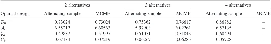
¼3;060 choice sets. The optimal designs from the alternating sample algorithm appear in Tables A.1, A.2, and A.3 of the Appendix. Table 1 compares the criterion values of these designs with the criterion values obtained by Kessels et al. (2006) using the MCMF algorithm. The two-alternative DB-optimal designs from both algorithms are equivalent.
However, in all the other cases with two and three alternatives, the designs generated with the alternating sample algorithm outperform the designs generated with MCMF.
The best criterion values from the alternating sample algo-rithm were the result of 1,000 random starts rather than the 200 random starts used to obtain the best criterion values from MCMF. Because the alternating sample algorithm is so much faster than MCMF, the extra random starts were still accom-plished using far less computing time. The computing times for one random start of the alternating sample algorithm and MCMF appear in Tables 2(a) and 2(b), respectively. We per-formed all computations in MATLAB 7 using a Dell personal computer with a 1.60 GHz Intel Processor and 2 GB RAM.
Tables 2(a) and 2(b) show the huge reductions in computing time using the alternating sample algorithm. Particularly important are the reductions in computing time for theGB- and VB-optimality criteria, which make the construction of GB
-and VB-optimal designs practically feasible. Even the
four-alternativeGB- andVB-optimal designs were generated quickly,
whereas their computation was not doable with MCMF. Notice also the faster running time for the VB-optimality criterion
compared with the GB-optimality criterion. This is due to a
computational short cut in the calculation of theVB-optimality
criterion, which we lay out in Section 4.3.
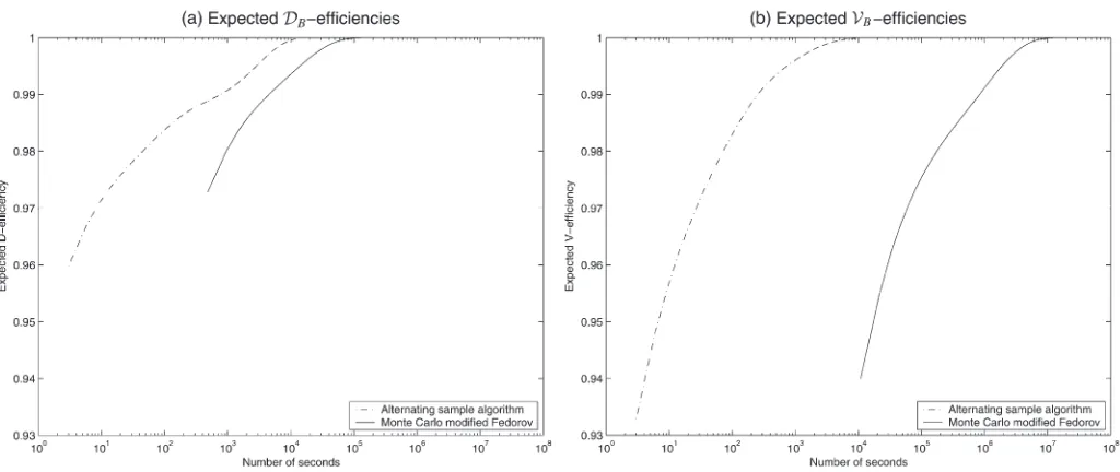
A comparison of the effectiveness of the alternating sample algorithm and MCMF appears in the plots of Figure 1. In these graphs, we plotted the estimated expected efficiencies of the two-alternative DB- and VB-optimal designs against the number of
seconds of computing time. We expressed the number of seconds on a log-scale. These plots provide compelling evidence of the practical value of the alternating sample algorithm. The huge increase in speed created by the alternating sample algorithm overtly leads to more efficient designs in a given amount of com-puting time. This is especially the case for the prediction-based design criteria as illustrated by the plot for theVB-efficiencies. Note
however, that the bend in the plot for theDB-efficiencies reveals
that the alternating sample algorithm has a little difficulty making the final jump from 99% efficiency to 100% or global efficiency. Details on the calculation of the expected efficiency from a number of random starts can be found in the work of Kessels et al. (2006). The plots for the two-alternativeDB- andVB-optimal designs
in Figure 1 are representative of the two-alternative AB- and GB-optimal designs, respectively. The plots for the
three-alternative designs exhibit a similar pattern.
4. FEATURES OF THE ALTERNATING SAMPLE ALGORITHM
There are four features of the alternating sample algorithm that result in increased speed compared with MCMF. In order of importance, they are
Table 1.DB-;AB-;GB-;andVB-criterion values of theDB-;AB-;GB-;andVB-optimal designs for the comparison example 3232/24 computed
using the alternating sample algorithm and the Monte Carlo modified Fedorov algorithm
Optimal design
2 alternatives 3 alternatives 4 alternatives
Alternating sample MCMF Alternating sample MCMF Alternating sample MCMF
DB 0.73024 0.73024 0.75362 0.76617 0.86782 –
AB 6.55212 6.60563 5.97903 6.02261 6.57135 –
GB 0.49887 0.51997 0.51051 0.51843 0.60494 –
VB 0.07184 0.07219 0.06267 0.06285 0.05728 –
1. a small designed sample of prior parameters, 2. a coordinate-exchange algorithm,
3. an efficient computation of theVB-optimality criterion, and
4. a fast update of the Cholesky decomposition of the information matrix.
The next sections discuss each of these in succession.
4.1 Small Designed Sample of Prior Parameters
In this section, we present a new method to approximate the integral related to a multivariate normal prior pðbÞ ¼ N ðbjb0;S0Þ in the definitions of the Bayesian optimality criteria. The solution of the integral with respect to a
multi-variate normal prior for the various criteria has not been accomplished analytically. In general, for models that are nonlinear in the parameters some numeric approximation to the integral is necessary (Chaloner and Verdinelli 1995).
Sa´ndor and Wedel (2001) and Kessels et al. (2006) used a Monte Carlo estimate of the integral from 1,000 random draws of the prior. By the law of large numbers, such estimates are known to converge to the true value of the integral at a rate proportional to the square root of the number of draws. This necessitates a large number of draws to reduce the sample-to-sample variability to the point where different sample-to-samples do not lead to different design choices. This approach is costly because the computing time for the Bayesian design is then roughly 1,000 times longer than the computing time for a locally optimal design (i.e., the design for one prior parameter vector).
To solve integrals related to a multivariate normal dis-tribution for the construction of choice designs, Sa´ndor and Wedel (2002) used samples based on orthogonal arrays (Tang 1993) and Sa´ndor and Wedel (2005) constructed quasi-Monte Carlo samples (Hickernell, Hong, L’Ecuyer, and Lemieux 2000). In several cases, estimates using these methods are more efficient than Monte Carlo estimates so that it is possible to employ smaller samples to obtain the same accuracy (Sa´ndor and Andra´s 2004; Sa´ndor and Train 2004). There is also an extensive literature on quadrature, which is another approach to numerical integration. One such work is Sloan and Joe (1994), who discussed good lattice point methods. However, for inte-grals of functions in more than four dimensions, Monte Carlo estimates tend to outperform quadrature estimates (Geweke 1996; Monahan and Genz 1997).
4.1.1 A Designed Set of Sample Parameters. We propose to approximate the integrals in (2), (3), (4), and (6) with a designed sample of only a small number of parameter vectors. Assuming that the prior variance-covariance matrix S0 is proportional to the identity matrix, the multivariate normal dis-tribution is spherically symmetric around the prior mean. As a result, every parameter has the same density on ak-dimensional Table 2. Computing times for one random start of the alternating
sample algorithm and the Monte Carlo modified Fedorov algorithm to generate the Bayesian optimal designs for the comparison example
3232/24.
(a) Alternating sample algorithm
Design criterion
# Alternatives
2 3 4
DB 00:00:03 00:00:04 00:00:05
AB 00:00:03 00:00:04 00:00:05
GB 00:00:07 00:00:32 00:04:23
VB 00:00:03 00:00:05 00:00:08
(b) Monte Carlo modified Fedorov
Design criterion
# Alternatives
2 3 4
DB 00:08:00 00:08:00 –
AB 00:08:00 00:08:00 –
GB 03:00:00 12:00:00 –
VB 03:00:00 12:00:00 –
NOTE: The times are expressed in hours:minutes:seconds.
Figure 1. Estimated expected efficiencies against computation time of the alternating sample algorithm and the Monte Carlo modified
Fedorov algorithm for producing the two-alternativeDB- andVB-optimal designs.
hypersphere of a given radius. The parameter vectors we use are uniformly distributed on such a sphere. In this way, they sample the different directions away from the prior mean fairly. The designed sample yields an approximation that is worse than the Monte Carlo sample of 1,000 draws. However, in the computation of Bayesian optimal designs, it is not necessary for the approximation of the integral to be accurate. All that is required is that the sign of the difference from a rough approximation corresponding to two slightly different designs matches the sign of the difference from a better approximation. In our examples, we chose 20 parameter vectors as a com-promise between computation time and precision of the inte-gral approximation. For the 32 3 2/24 example, the plot in Figure 2 illustrates that the systematic sample and the Monte Carlo sample largely agree on design improvements in a ran-dom start of the alternating sample algorithm.
The plot compares the VB-criterion value for the Monte
Carlo sample with theVB-criterion value for the systematic
20-point sample. It depicts the course of one random start of the coordinate-exchange algorithm for the two-alternative designs. From a random starting design, the algorithm makes a sequence of changes, each of which improves theVB-criterion
value for the systematic 20-point sample. By reevaluating each of these changes with the VB-criterion value for the Monte
Carlo sample, we find out whether every change also leads to an improvement using the better approximation.
The starting design is represented by the point at the top right of the plot, which of all points has the highest or worstVB
-criterion value according to the 20-point sample as well as the Monte Carlo sample. After making one change in the original design, the second point from the top right shows an improvement in theVB-criterion value for both samples. The
points proceed from the top right to the bottom left of the plot. The point at the bottom left denotes the final and best design produced in the random start. Note that this point has the lowest
or best VB-criterion value as approximated by both samples.
Furthermore, note that the drop in theVB-criterion value is not
monotonic, indicating that the two approximations are not in complete agreement about the VB-criterion value of each
change in the sequence.
Still, the agreement between the VB-criterion value for the
Monte Carlo sample and the VB-criterion value for the
sys-tematic 20-point sample is clear from a correlation of 99%. Similar correlations are obtained using the coordinate-exchange algorithm with every other design criterion and with larger choice set sizes. However, this does not imply that designs that are optimal using the systematic 20-point sample are also optimal with respect to the Monte Carlo sample. The plot in Figure 3 demonstrates this.
Like the plot in Figure 2, the plot in Figure 3 displays theVB
-criterion value for the Monte Carlo sample versus theVB-criterion
value for the systematic 20-point sample. Now each point in the plot represents the best two-alternative design found in a single random start of the coordinate-exchange algorithm. Again, the algorithm used theVB-criterion value for the 20-point sample to
generate the designs and the VB-criterion value for the Monte
Carlo sample to reevaluate them. From the plot, we see that the worst design by both VB-criterion values is the same. On the
other hand, the best design according to theVB-criterion value
for the 20-point sample differs from the best design indicated by theVB-criterion value for the Monte Carlo sample.
In this case, the correlation between theVB-criterion values
for the Monte Carlo sample and theVB-criterion values for the
20-point sample from the different random starts is only 66%. This result also applies to the other design criteria and larger choice set sizes. The fact that the correlation is not close to 100% means that it is important to reevaluate the design pro-duced by the algorithm after each random start with one cal-culation of the objective function using the Monte Carlo sample. Therefore, our approach alternates between the small
Figure 2. VB-criterion values according to the 1,000-point Monte
Carlo sample versus the systematic 20-point sample and correlation between them. The points represent the course of one random start of the coordinate-exchange algorithm for the two-alternative designs using the 20-point sample.
Figure 3.VB-criterion values according to the 1,000-point Monte
Carlo sample versus the systematic 20-point sample and correlation between them. Each point represents a design produced from a dif-ferent random start of the coordinate-exchange algorithm.
designed sample and the large Monte Carlo sample. Ultimately, the design with the best criterion value in terms of the Monte Carlo sample is selected.
Note that, if the correlation were near 100%, it would not be necessary to check the designs. Also, observe that because of the decrease in the number of prior parameters from 1,000 to 20 during a random start we save up to 98% of the computa-tional work.
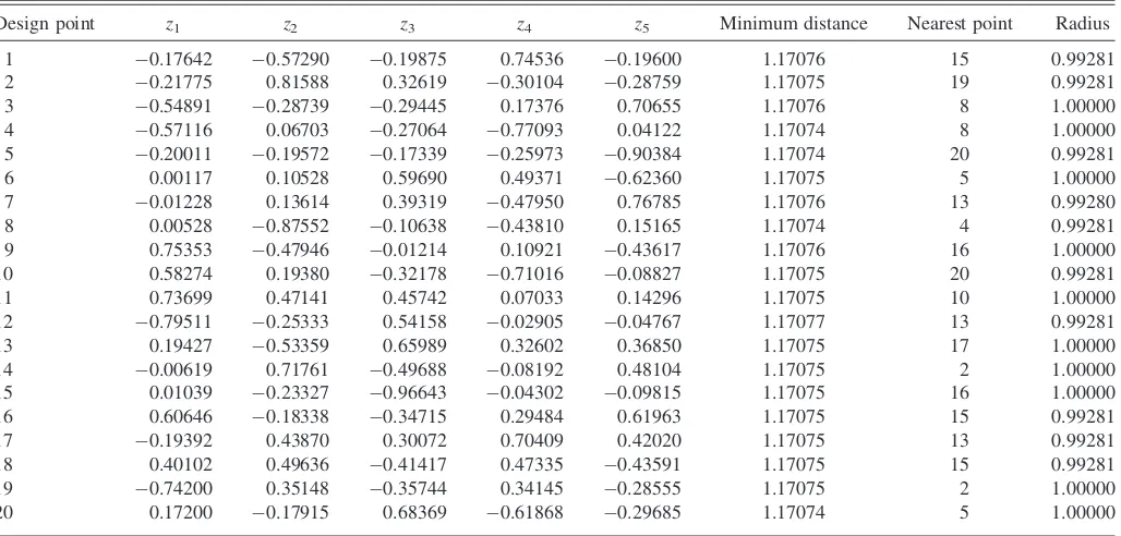
4.1.2 Constructing a Small Sample of Prior Parameters. For any choice design problem, we can construct a small set of prior parameters using a minimum potential design (see SAS 2007, pp. 160–161). These designs were created using the commercial software JMP 7. For dimensions larger than three, the points of these designs will be uniformally distributed on a k-dimensional hypersphere at a radius of one away from the zero vector. So on the sphere, the minimum distance to a neighboring point from any of the design points will be roughly the same for all the points.
To understand how minimum potential designs are created, consider n points on a k-dimensional sphere around the zero vector. Each point,p, is labeled (zp1,. . .,zpk). Let def be the
distance between theeth andfth points. That is
def ¼
The optimization problem is to find then3kvalues ofzpithat
minimizeEpot, the potential energy of the system:
Epot¼
In this expression, imagine the n points as electrons with springs attached to every point. Then,d2efis proportional to the energy stored in a spring when you pull it and 1/def is the
potential energy between two electrons. When the distance
between two points increases,d2efincreases. When the distance between two points decreases, 1/defincreases.
For the comparison example, the minimum potential design with 20 points in a 5-dimensional space appears in Table 3. These points lie on a sphere of a radius of one around [0, 0, 0, 0, 0]9. The minimum distance for each point to the nearest point is 1.171. If this interpoint distance seems too large, then it can be reduced by increasing the number of points.
To properly approximate the prior distribution with a 20-point sample from the 20-points of a minimum potential design, it is necessary to rescale these points for the prior variance-covariance matrix and the prior mean. If there is no correlation between the prior coefficients orS0¼s20Ik;then the 20-point
sample lies on a sphere with a radius that is proportional to the standard deviations0. Now, the effectiveness of the 20-point
sample in the alternating sample algorithm depends on the radius specified, or the number of standard deviations away from the prior mean. That is to say, a well-chosen radius requires fewer random starts to reach the global optimum. To find the best radius for a spherical 20-point sample for any choice design problem, one could proceed as follows:
1. Do a number of random starts of the alternating sample algorithm for each of three radii.
2. Fit a quadratic function to the minimum criterion value found at each radius.
3. Choose the radius that minimizes the quadratic function.
For the comparison example, we performed 10 random starts for a radius of 1, 2, and 3. Recall thats0¼1 for this example.
The result for theVB-optimality criterion connected with
two-alternative designs appears in Figure 4. Fitting a quadratic model to the minima results in a radius slightly larger than 2. We chose, however, a radius of 2 for simplicity. To illustrate the value of selecting a good radius, we compared the esti-mated expected efficiencies per number of random starts of the
Table 3. Minimum potential design of 20 points in 5 continuous factors for the comparison example.
Design point z1 z2 z3 z4 z5 Minimum distance Nearest point Radius
1 0.17642 0.57290 0.19875 0.74536 0.19600 1.17076 15 0.99281
2 0.21775 0.81588 0.32619 0.30104 0.28759 1.17075 19 0.99281
3 0.54891 0.28739 0.29445 0.17376 0.70655 1.17076 8 1.00000
4 0.57116 0.06703 0.27064 0.77093 0.04122 1.17074 8 1.00000
5 0.20011 0.19572 0.17339 0.25973 0.90384 1.17074 20 0.99281
6 0.00117 0.10528 0.59690 0.49371 0.62360 1.17075 5 1.00000
7 0.01228 0.13614 0.39319 0.47950 0.76785 1.17076 13 0.99280
8 0.00528 0.87552 0.10638 0.43810 0.15165 1.17074 4 0.99281
9 0.75353 0.47946 0.01214 0.10921 0.43617 1.17076 16 1.00000
10 0.58274 0.19380 0.32178 0.71016 0.08827 1.17075 20 0.99281
11 0.73699 0.47141 0.45742 0.07033 0.14296 1.17075 10 1.00000
12 0.79511 0.25333 0.54158 0.02905 0.04767 1.17077 13 0.99281
13 0.19427 0.53359 0.65989 0.32602 0.36850 1.17075 17 1.00000
14 0.00619 0.71761 0.49688 0.08192 0.48104 1.17075 2 1.00000
15 0.01039 0.23327 0.96643 0.04302 0.09815 1.17075 16 1.00000
16 0.60646 0.18338 0.34715 0.29484 0.61963 1.17075 15 0.99281
17 0.19392 0.43870 0.30072 0.70409 0.42020 1.17075 13 0.99281
18 0.40102 0.49636 0.41417 0.47335 0.43591 1.17075 15 0.99281
19 0.74200 0.35148 0.35744 0.34145 0.28555 1.17075 2 1.00000
20 0.17200 0.17915 0.68369 0.61868 0.29685 1.17074 5 1.00000
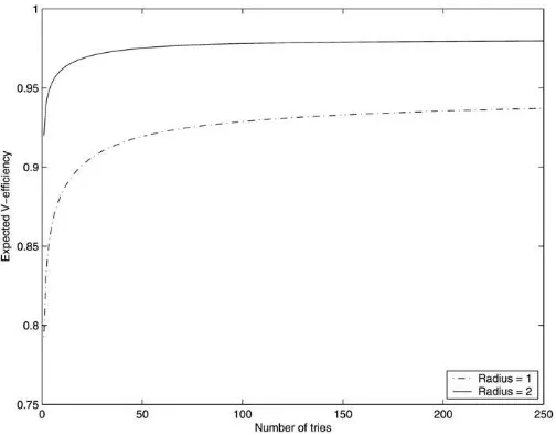
two-alternativeVB-optimal designs using the 20-point samples
for radii 1 and 2, respectively. The plots based on 250 random starts appear in Figure 5. We clearly observe the higher expected efficiencies in case a radius of 2 is used as opposed to a radius of 1. We obtained similar results for any other opti-mality criterion in combination with any choice set size.
However, computing the ‘‘best’’ radius is not absolutely necessary. The heuristic of choosing a sphere radius that is twice the prior standard deviation worked well in all the examples we tried. The critical part of the alternating sample algorithm is that for each random start using the 20-point sample, one checks the resulting design with the larger Monte Carlo sample. So, no matter what radius one chooses, one will have a monotonically improving set of designs as the number
of random starts increases. Still, choosing a good radius increases the speed of the improvement over the random starts.
4.2 Coordinate-Exchange Algorithm
The alternating sample algorithm uses Meyer and Nachts-heim’s (1995) coordinate-exchange algorithm to generate Bayesian optimal designs. The coordinate-exchange algorithm has also been applied by Kuhfeld and Tobias (2005) to generate D-efficient factorial designs for large choice experiments based on a linear model. As opposed to the modified Fedorov algo-rithm employed in Kessels et al. (2006), it allows the compu-tation of choice designs with a large number of profiles, attributes, and/or attribute levels in a reasonable amount of time. The coordinate-exchange algorithm can be seen as a greedy profile exchange algorithm. Whereas the modified Fedorov algorithm possibly changes every ‘‘coordinate’’ or attribute level of a profile, the coordinate-exchange algorithm only changes one coordinate at a time. For each attribute level in the design, the coordinate-exchange algorithm tries all possible levels and chooses the level corresponding to the best value of the optimality criterion under consideration.
The algorithm begins by creating a random starting design. Improvements are made to the starting design by considering changes in the design on an attribute-by-attribute basis. For any attribute of a given profile in the current design, the objective function is evaluated over all the levels of that attribute. If the maximal value of the objective function is larger than the current maximum, then the current maximum is replaced and the profile’s current attribute level is replaced by the new level corresponding to the maximal value of the objective function. This attribute-by-attribute procedure continues until a com-plete cycle through the entire design is comcom-pleted. Then, another complete cycle through the design is performed noting if any attribute level changes in the current pass. This continues until no changes are made in a whole pass or until a specified maximum number of passes have been executed.
In contrast with the modified Fedorov algorithm, the coor-dinate-exchange algorithm is a candidate-set-free algorithm. That is, it does not require the specification of a set of candidate profiles. This aspect becomes more important when the can-didate set is very large because of a large number of attributes and/or attribute levels. The coordinate-exchange algorithm is also substantially faster than the modified Fedorov algorithm. It runs in polynomial time, whereas the modified Fedorov algo-rithm runs in exponential time. For the comparison example, this leads to roughly a factor of three speed increase of the coor-dinate-exchange algorithm over the modified Fedorov algo-rithm. For designs with more profiles, attributes, and/or attribute levels, this increase in speed becomes more pronounced.
4.3 Efficient Computation of theVB-Optimality Criterion
In the alternating sample algorithm, the VB-optimality
criterion is implemented in an efficient way. For each prior vector of coefficients, it is possible to compute the average prediction variance without first computing the prediction variances for each profile xjq 2x separately. A similar
ap-proach does not apply to theGB-optimality criterion because
Figure 4. VB-criterion values of two-alternative designs from 10
random starts of the alternating sample algorithm using the 20-point samples for radii 1, 2, and 3.
Figure 5. Estimated expected efficiencies per number of random starts
of the two-alternativeVB-optimal designs computed using the
alternat-ing sample algorithm with the 20-point samples for radii 1 and 2.
finding the worst prediction variance requires the computa-tion of all variances.
The prediction variance on the left of (9) is naturally a scalar sincec(xjq) is ak31 vector andM
1a
k3kmatrix. The trace of a scalar is the scalar itself so that
c0 xjq ABC is a square matrix and the matrix product CAB exists. This equality is known as the cyclic property of the trace. Since the prediction variance is a scalar andc(xjq)c9(xjq) is ak3k
matrix that conforms withM1,
tr c0 xjq
be computed once for each prior parameter vector. We now average the individual matrices Wjqover all profiles xjq2x
and denote the subsequent matrix byW:
W¼ 1
The average prediction variance across all profilesxjq2xfor a
given prior parameter vector is then
ð
x
c0ðxjqÞM1cðxjqÞdxjq¼trðWM1Þ ð12Þ
We refer to the work of Meyer and Nachtsheim (1995) for a similar expression of the V-optimality criterion in the linear design setting.
So, to obtain the VB-optimality criterion, we have to
com-puteWfor each prior parameter vector only once. The set ofW matrices can be reused from one random start to the next.
4.4 Updating the Cholesky Decomposition of the Information Matrix
Updating the Cholesky decomposition of the information matrix is an economical way to compute theDB-;AB-;GB-;and VB-criterion values of designs that differ only in one profile,
and therefore one choice set, from another design. This is the case in the alternating sample algorithm, where at each step a new design is created by changing only one attribute level of a single profile (see Section 4.2).
IfM is a symmetric positive definite matrix, then its Cho-lesky decomposition is defined as
M¼L0L; ð13Þ
where L is an upper triangular matrix named the Cholesky factor. Note that the information matrix M is symmetric because it is the sum [from Equation (1)] of the information matrices of theS choice setsMs that are symmetric. Each of
these Ms is of the form X9sCsXs, where Cs ¼Ps psp9s is
symmetric.
We compute the DB-;AB-;GB-;and VB-criterion values of
each of the designs as follows. For each prior parameter vector, we compute the information matrixMthrough (1) and derive
its Cholesky factor L. We update the Cholesky factor after every profile change with low rank updates based on the work of Bennett (1965) and implemented in the MATLAB function CHOLUPDATE. The update is low rank because only one choice set is changing at any step.
Using the Cholesky factors the four criterion values for each design can be obtained as shown below. In this way, we avoid recomputation of the information matrix through (1). For the comparison example 32 3 2/24, this procedure reduced the computing times by roughly a factor of three.
We now illustrate how the different design criteria rely on the Cholesky factorL of the information matrixM. For any parameter vectorbr, theD-optimality criterion becomes
D ¼ ðdetðM1ÞÞ1=k¼1=ðdetðMÞÞ1=k
wherelii is theith diagonal element ofL. Thus, to obtain the
DB-criterion value of a design in which a profile has been
changed, we do not need to recompute the information matrix for every prior parameter vector. Only an update of the Cho-lesky factor is required.
To show the dependency of theAB-;GB-;andVB-optimality
criteria on the Cholesky factorL, the Cholesky decomposition (13) has to be inverted. The inverse is given by
M1¼ ðL0LÞ1¼L1L1 9
: ð15Þ
Because the Cholesky factor, L, is triangular, inverting it is easier than invertingM. Then, for any prior parameter vector, theA-optimality criterion is
A ¼trðM1Þ ¼trL1L1 9¼X
criterion value of a design in which a profile has been changed, we need to derive the new Cholesky factor for every prior parameter vector and take its inverse. This goes much faster than computing the new information matrix and inverting it.
In a similar manner, the GB- and VB-criterion values are
obtained. The prediction variance of profilexjq2xis expressed as
c0ðxjqÞM1cðxjqÞ ¼c0ðxjqÞL1 L1
9
cðxjqÞ: ð17Þ
Here,c(xjq) does not depend on the designXand therefore only
needs to be computed once for each prior parameter vector. The GB-criterion value is obtained by inserting (17) in (4). For the VB-optimality criterion, we performed some initial calculations
that make its computation even more efficient as discussed previously.
5. DESIGNING A FOLLOW UP EXPERIMENT
The speed of the alternating sample algorithm makes the computation of Bayesian optimal designs feasible for more challenging problems of larger dimensions than the rather small comparison example 32 3 2/24. We illustrate this with the construction of a follow up design to the choice experiment on
sports club membership described in Sa´ndor and Wedel (2001) and carried out at the University of Groningen in the Nether-lands. The original experiment consisted of 30 choice sets of size two, half of which were obtained using the BayesianD -opti-mality criterion. The other 15 choice sets formed a non-Baye-sianD-optimal design. The Bayesian and the non-BayesianD -optimal design are displayed in Table A.4. The two designs were presented to each of the respondents in one session. The order of presentation of the choice sets from each design was alternated. The profiles in the experiment were configured from five three-level attributes. So in total, there are 35¼243 candidate profiles. This candidate set is much larger than the candidate set of 18 profiles employed in the comparison example.
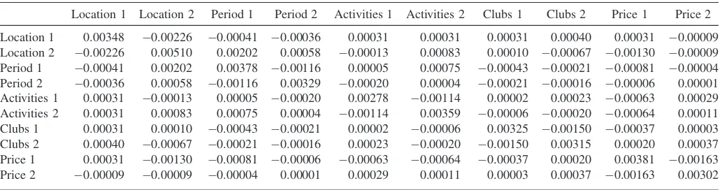
We acquired data from 43 of the original 58 respondents from the authors of the original study, and analyzed it using the NLPCG subroutine in SAS. The parameter estimates and standard errors we obtained are given in Table 4. The var-iance-covariance matrix of the estimates is displayed in Table 5. We used the parameter estimates and their variance-cova-riance matrix as the mean and vavariance-cova-riance of the multivariate normal prior distributionpðbÞwhen designing the follow up study. We denote the vector of parameter estimates, which serves as the prior mean, byb0, and its covariance matrix byS0. The procedure required to useb0as the prior mean andS0as the prior variance in the alternating sample algorithm is as follows. First, randomly generate 1,000 parameter vectors from the standard normal distribution. If we denote any of these vectors byn, then a random parameter vectorbr drawn from the multivariate normal distribution with meanb0and variance S0can be constructed using
br¼b0þD0n; ð18Þ
where D is the Cholesky factor of the variance-covariance matrixS0, so thatD9D¼S0.
Creating the designed sample of 20 parameter vectors using a minimum potential design and multiplying by 2 will put these vectors on the surface of a hypersphere of radius 2. Pre-multiplying the resulting vectors by the transpose of the Cholesky factor,D9, moves them to the surface of a hyperellipsoid. This makes them have approximately the same correlation structure as the previously described Monte Carlo sample, because the minimum potential design is always nearly orthogonal. That is, the inner product of differing pairs of columns is close to zero. Finally, the designed sample needs to be recentered to the prior mean vectorb0 by addingb0to the outcome of the premultiplication byD9.
We assumed that the original respondents were contacted for the follow up study and that they were asked to evaluate 10 additional choice sets. Together with the 30 choice sets of the original study, these choice sets make up the augmented design. We have constructed optimal follow up designs using theDB
-and VB-optimality criteria and 1,000 random starts of the
alternating sample algorithm. For this problem, x consists of Q¼2432 ¼29;403 choice sets. The DB- and VB-optimal
follow up designs are displayed in Table A.5 of the Appendix. Table 6 shows the improvement in terms of estimation and prediction capability, as measured by theDB- andVB-criteria,
due to the additional choice sets. The criteria depend on the prior mean vector,b0, and variance-covariance matrix,S0, in Table 4 and Table 5, respectively. As can be seen from theDB-criterion
values, theDB- andVB-optimal augmented designs are nearly
equivalent in terms of precision of estimation. TheVB-optimal
design is slightly moreVB-efficient than theDB-optimal design.
In this application, the practical difference between theDB
-and VB-optimal designs is minuscule. To check whether this
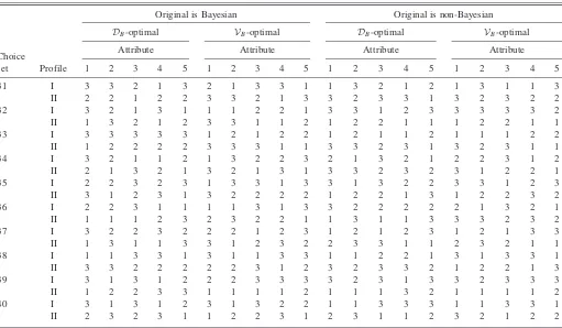
result also holds in case of a smaller original design, we computedDB- andVB-optimal follow up designs of 10 choice
sets both for the 15 choice sets of the Bayesian and the non-BayesianD-optimal design. These follow up designs appear in Table A.6 of the Appendix and theDB- andVB-criterion values
of the augmented designs are given in Table 7. Although the differences in DB-efficiency and VB-efficiency are larger for
these smaller design cases, we cannot conclude that there is any practical distinction between theDB- andVB-optimal designs.
Table 4. Parameter estimates and standard errors for the sports club membership choice experiment in Sa´ndor and Wedel (2001)
Coefficient Estimates Standard error
Location 1 0.58 0.059
Location 2 0.90 0.071
Period 1 0.63 0.061
Period 2 0.05 0.057
Activities 1 0.03 0.053
Activities 2 0.35 0.060
Clubs 1 0.15 0.057
Clubs 2 0.36 0.056
Price 1 0.54 0.062
Price 2 0.02 0.055
Table 5. Variance-covariance matrix of the parameter estimates for the sports club membership choice experiment in Sa´ndor and Wedel (2001)
Location 1 Location 2 Period 1 Period 2 Activities 1 Activities 2 Clubs 1 Clubs 2 Price 1 Price 2
Location 1 0.00348 0.00226 0.00041 0.00036 0.00031 0.00031 0.00031 0.00040 0.00031 0.00009
Location 2 0.00226 0.00510 0.00202 0.00058 0.00013 0.00083 0.00010 0.00067 0.00130 0.00009
Period 1 0.00041 0.00202 0.00378 0.00116 0.00005 0.00075 0.00043 0.00021 0.00081 0.00004
Period 2 0.00036 0.00058 0.00116 0.00329 0.00020 0.00004 0.00021 0.00016 0.00006 0.00001
Activities 1 0.00031 0.00013 0.00005 0.00020 0.00278 0.00114 0.00002 0.00023 0.00063 0.00029
Activities 2 0.00031 0.00083 0.00075 0.00004 0.00114 0.00359 0.00006 0.00020 0.00064 0.00011
Clubs 1 0.00031 0.00010 0.00043 0.00021 0.00002 0.00006 0.00325 0.00150 0.00037 0.00003
Clubs 2 0.00040 0.00067 0.00021 0.00016 0.00023 0.00020 0.00150 0.00315 0.00020 0.00037
Price 1 0.00031 0.00130 0.00081 0.00006 0.00063 0.00064 0.00037 0.00020 0.00381 0.00163
Price 2 0.00009 0.00009 0.00004 0.00001 0.00029 0.00011 0.00003 0.00037 0.00163 0.00302
We note, however, that theDB- andVB-criterion values of the
designs match those of the larger original design shown in Table 6. The augmented designs use only 25 choice sets, whereas the larger original design has 30 choice sets. This shows the value of augmenting a small initial conjoint choice design, which allows one to update the knowledge about the unknown model parameters before spending all experimental resources.
6. CONCLUSION
In this article, we propose an alternating sample algorithm for producingDB-;AB-;GB-;andVB-optimal choice designs as
an alternative to the MCMF algorithm employed by Kessels et al. (2006). Kessels et al. (2006) had shown thatGB- andVB
-optimal designs outperform DB- and AB-optimal designs for
response prediction, which is central in choice experiments. However, using the MCMF algorithm for computingGB- and VB-optimal designs is even more cumbersome than searching
for DB- and AB-optimal designs so that they suggested
implementing theDB-optimality criterion in practice.
Unlike the MCMF algorithm, the new alternating sample algorithm makes the construction of GB- and VB-optimal
designs practical and it allows the DB-;AB-;GB-; and VB
-optimal designs to be embedded in web-based conjoint choice studies with individualized designs for the respondents. We prefer using VB-optimal designs because they minimize the
average prediction variance and can be computed faster than GB-optimal designs. In general, the main improvement of the
alternating sample algorithm over the MCMF algorithm is the approximation of the normal prior distribution by a designed sample of 20 parameter vectors instead of a Monte Carlo sample of 1,000 random draws. This saves up to 98% of the computational work within each random start of the algorithm. Nevertheless, we reevaluate the designs produced by each random start using the Monte Carlo sample and adapt the
design selection accordingly. This led us to call our method the alternating sample algorithm.
To further speed up the design generation, the alternating sample algorithm also uses a coordinate-exchange algorithm rather than a modified Fedorov algorithm. A coordinate-exchange approach saves time by avoiding the creation and use of a candidate set that grows exponentially with the number of attributes and attribute levels studied. Thus, the time savings of the coordinate-exchange algorithm increase with the number of profiles, attributes, and attribute levels. As a last way to accelerate the computations for any optimality criterion, the alternating sample algorithm incorporates an update formula to economically calculate the information matrix and the opti-mality criterion values of designs.
We also show how correlations between the parameter coefficients can be taken into account when computing the optimal choice designs. In case one suspects such correlations to be present, the multivariate normal prior distribution is elliptically symmetric around the prior mean. The small designed sample of parameters from a minimum potential design can then be linearly transformed to lie on the appro-priatek-dimensional ellipsoid.
The computational speed of the alternating sample algo-rithm makes the use of individualized, adaptive Bayesian optimal conjoint choice designs in web-based surveys possi-ble. Such an approach would involve generating an initial design for each respondent using one of the Bayesian opti-mality criteria, and augmenting that design choice set by choice set for each respondent individually exploiting the information contained within the choices made by that respondent in the course of the experiment. The procedure for augmenting an existing design outlined in Section 5 lends itself to be implemented in such a framework for creating individ-ualized designs. To examine what is the best way to do this is, however, beyond the scope of this article. We expect that such an approach would allow an efficient estimation of mixed logit (Sa´ndor and Wedel 2002) and latent class models (Andrews, Ainslie, and Currim 2002; Train 2003) that aim at modeling consumer heterogeneity. A related avenue for future research is to explore strategies for two-stage optimal choice experiments. One such strategy could be to use theDB-optimality criterion to
design a pilot study, where the goal would be to get precise parameter estimates that can be used as prior information for the design of a follow up study. For the design of that follow up study, the use of the VB-optimality criterion might be more
appropriate because the goal is typically to make predictions. Also, the efficiency of optimal designs with respect to the choice set size might be further investigated.
The alternating sample algorithm and all designs discussed in the article can be downloaded from the following URL: http://www.ua.ac.be/Peter.Goos.
ACKNOWLEDGMENTS
We thank the two referees for suggesting the extension of the original method to apply to correlated priors. We also thank Prof. Hans Nyquist for hosting the first author for six weeks at the Department of Statistics of the University of Stockholm, Sweden, while she was working on this article.
Table 6.DB- andVB-criterion values for the original and the
augmented designs for the sports club membership study
Design DB-criterion VB-criterion
Original 0.12193 0.05103
DB-optimal augmented 0.08120 0.03263
VB-optimal augmented 0.08121 0.03240
Table 7.DB- andVB-criterion values for the smaller original designs
and the augmented designs for the sports club membership study
Design
Original is Bayesian
Original is non-Bayesian
DB-criterion VB-criterion DB-criterion VB-criterion
Original 0.27976 0.15158 0.31415 0.40521
DB-optimal
APPENDIX: CHOICE DESIGN TABLES
Table A.1. Two-alternative Bayesian optimal designs for the 32
32/24
Table A.2. Three-alternative Bayesian optimal designs
for the 32
Table A.3. Four-alternative Bayesian optimal designs
for the 3232/24 example
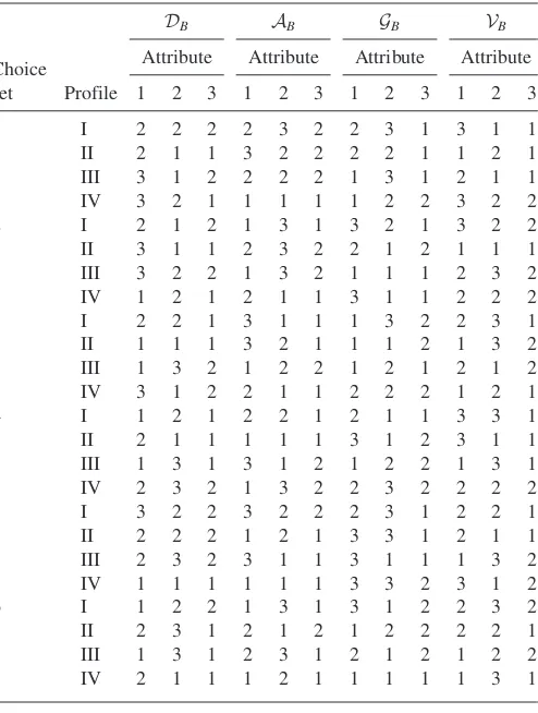
Table A.4. Bayesian and non-BayesianD-optimal designs with 15
choice sets used by Sa´ndor and Wedel (2001) for the sports club membership example
Table A.4. Continued
Non-Bayesian design Bayesian design
Choice
set Profile
Attribute
Choice set Profile
Attribute
1 2 3 4 5 1 2 3 4 5
9 I 2 1 3 2 3 10 I 2 2 1 2 2
II 1 2 2 3 1 II 1 3 3 3 1
11 I 3 2 1 3 1 12 I 1 2 3 1 1
II 1 3 3 2 3 II 3 3 1 3 3
13 I 2 2 3 1 2 14 I 1 2 1 1 2
II 1 3 1 2 1 II 2 3 3 2 1
15 I 1 1 3 2 2 16 I 2 3 1 1 2
II 3 3 2 1 3 II 3 2 3 2 3
17 I 3 2 1 1 2 18 I 1 1 3 3 2
II 2 3 2 3 1 II 2 2 1 1 1
19 I 1 3 2 2 2 20 I 2 3 3 2 2
II 2 1 3 1 1 II 1 1 2 1 1
21 I 2 2 1 2 1 22 I 3 2 1 2 1
II 3 1 2 3 3 II 2 3 2 1 3
23 I 3 1 1 1 1 24 I 3 1 2 2 1
II 1 2 3 3 3 II 1 2 3 3 3
25 I 2 3 1 3 2 26 I 2 3 2 3 2
II 3 1 2 2 3 II 3 1 1 2 3
27 I 1 2 3 1 1 28 I 2 1 1 1 1
II 3 1 1 3 2 II 3 2 2 3 2
29 I 3 1 2 1 2 30 I 1 2 3 2 2
II 2 3 1 3 3 II 3 1 2 3 3
Table A.6.DB-andVB-optimal follow up designs for the isolated Bayesian and non-BayesianD-optimal designs of Table A.4 used in the sports
club membership example
Original is Bayesian Original is non-Bayesian
DB-optimal VB-optimal DB-optimal VB-optimal
Choice
set Profile
Attribute Attribute Attribute Attribute
1 2 3 4 5 1 2 3 4 5 1 2 3 4 5 1 2 3 4 5
31 I 3 3 2 1 3 2 1 3 3 1 1 3 2 1 2 1 3 1 1 3
II 2 2 1 2 2 3 3 2 1 3 3 2 3 3 1 3 2 3 2 2
32 I 3 2 1 3 1 1 1 2 2 1 3 3 1 2 3 3 3 3 3 2
II 1 3 2 1 2 3 3 1 1 2 1 2 2 1 1 1 2 2 1 1
33 I 3 3 3 3 3 1 2 1 2 2 1 2 1 1 2 1 1 1 2 2
II 1 2 2 2 2 3 3 3 1 1 3 3 2 3 1 3 2 3 1 1
34 I 3 2 1 1 2 1 3 2 2 3 2 1 3 2 1 2 2 3 1 2
II 2 1 3 2 1 3 2 1 3 1 3 3 2 3 2 3 1 2 2 1
35 I 2 2 3 2 3 1 3 3 1 3 3 1 3 2 2 3 3 1 2 3
II 3 1 2 3 1 3 2 2 2 2 1 2 2 1 3 1 2 2 3 2
36 I 2 2 3 1 1 1 1 3 1 3 3 2 2 2 2 2 1 3 2 1
II 1 1 1 2 3 2 3 2 2 1 1 3 1 1 3 3 3 2 3 2
37 I 3 2 2 3 2 2 2 1 2 3 1 2 1 2 3 1 2 1 3 3
II 1 3 1 1 3 3 1 2 3 2 2 3 3 1 1 2 3 2 1 1
38 I 1 1 3 3 1 3 1 1 3 3 1 1 2 2 1 3 1 3 3 1
II 3 3 2 2 2 2 2 3 1 2 3 2 3 3 2 1 2 2 1 3
39 I 3 1 3 1 2 2 2 3 3 3 3 2 3 1 3 3 2 3 3 3
II 1 2 2 3 3 1 1 1 1 2 1 1 1 3 2 1 1 1 1 2
40 I 3 1 3 1 2 3 1 3 2 2 1 1 3 3 3 1 1 3 3 1
II 2 3 2 3 1 1 2 2 3 1 2 3 1 1 2 3 2 1 2 2
Table A.5.DB- andVB-optimal follow up designs for the combined
Bayesian and non-BayesianD-optimal design of Table A.4 used in the
sports club membership example.
DB-optimal VB-optimal
Choice
set Profile
Attribute Attribute
1 2 3 4 5 1 2 3 4 5
31 I 3 3 3 3 3 1 1 2 2 2
II 1 2 1 1 2 3 3 3 1 3
32 I 1 2 3 1 1 3 3 3 1 2
II 3 3 1 2 2 1 2 1 2 3
33 I 1 1 1 3 3 3 3 1 3 3
II 2 2 2 2 2 2 2 3 1 1
34 I 3 3 2 1 1 1 1 2 3 1
II 1 2 1 2 3 3 2 1 1 2
35 I 1 2 2 3 1 3 2 2 3 1
II 3 3 3 1 2 1 1 1 2 2
36 I 2 1 3 2 1 2 2 3 3 1
II 3 2 2 3 2 1 3 2 1 3
37 I 2 2 3 3 1 1 3 2 1 1
II 1 1 2 2 2 3 2 3 2 2
38 I 1 3 2 1 3 3 2 2 3 2
II 3 1 3 3 1 2 3 3 1 3
39 I 1 3 1 1 3 3 3 2 2 2
II 3 2 3 3 2 1 2 3 3 3
40 I 3 2 3 1 3 1 2 2 1 2
II 1 1 2 3 1 3 1 3 3 1
[Received October 2006. Revised November 2007.]
REFERENCES
Andrews, R. L., Ainslie, A., and Currim, I. S. (2002), ‘‘An Empirical Comparison of Logit Choice Models with Discrete Versus Continuous Representations of Heterogeneity,’’Journal of Marketing Research, 39, 479–487.
Bennett, J. M. (1965), ‘‘Triangular Factors of Modified Matrices,’’Numerische Mathematik, 7, 217–221.
Chaloner, K., and Verdinelli, I. (1995), ‘‘Bayesian Experimental Design: A Review,’’Statistical Science, 10, 273–304.
Cook, R. D., and Nachtsheim, C. J. (1980), ‘‘A Comparison of Algorithms for Constructing ExactD-Optimal Designs,’’Technometrics, 22, 315–324. Fedorov, V. V. (1972),Theory of Optimal Experiments, New York: Academic Press. Geweke, J. (1996), ‘‘Monte Carlo Simulation and Numerical Integration’’, in Handbook of Computational Economics(Vol. 1, Chap. 15), eds. H. M. Amman, D. A. Kendrick, and J. Rust, Amsterdam: Elsevier Science, pp. 731–800.
Hickernell, F. J., Hong, H. S., L’Ecuyer, P., and Lemieux, C. (2000), ‘‘Exten-sible Lattice Sequences for Quasi-Monte Carlo Quadrature,’’SIAM Journal on Scientific Computing, 22, 1117–1138.
Huber, J., and Zwerina, K. (1996), ‘‘The Importance of Utility Balance in Efficient Choice Designs,’’Journal of Marketing Research, 33, 307–317. Kessels, R., Goos, P., and Vandebroek, M. (2006), ‘‘A Comparison of Criteria to
Design Efficient Choice Experiments,’’Journal of Marketing Research, 43, 409–419.
Kuhfeld, W. F., and Tobias, R. D. (2005), ‘‘Large Factorial Designs for Product Engineering and Marketing Research Applications,’’Technometrics, 47, 132–141. Meyer, R. K., and Nachtsheim, C. J. (1995), ‘‘The Coordinate-Exchange Algorithm for Constructing Exact Optimal Experimental Designs,’’ Tech-nometrics, 37, 60–69.
Monahan, J., and Genz, A. (1997), ‘‘Spherical-Radial Integration Rules for Bayesian Computation,’’Journal of the American Statistical Association, 92, 664–674.
Sa´ndor, Z., and Andra´s, P. (2004), ‘‘Alternative Sampling Methods for Esti-mating Multivariate Normal Probabilities,’’Journal of Econometrics, 120, 207–234.
Sa´ndor, Z., and Train, K. (2004), ‘‘Quasi-Random Simulation of Discrete Choice Models,’’Transportation Research B, 38, 313–327.
Sa´ndor, Z., and Wedel, M. (2001), ‘‘Designing Conjoint Choice Experiments Using Managers’ Prior Beliefs,’’Journal of Marketing Research, 38, 430–444. Sa´ndor, Z., and Wedel, M. (2002), ‘‘Profile Construction in Experimental
Choice Designs for Mixed Logit Models,’’Marketing Science, 21, 455–475. Sa´ndor, Z., and Wedel, M. (2005), ‘‘Heterogeneous Conjoint Choice Designs,’’
Journal of Marketing Research, 42, 210–218.
SAS (2007),JMP Design of Experiments Guide(Release 7), SAS Institute Inc., Cary, NC, USA.
Sloan, I. H., and Joe, S. (1994),Lattice Methods for Multiple Integration, Oxford, U.K.: Oxford University Press.
Tang, B. (1993), ‘‘Orthogonal Array-Based Latin Hypercubes,’’Journal of the American Statistical Association, 88, 1392–1397.
Train, K. E. (2003),Discrete Choice Methods with Simulation, Cambridge, U.K.: Cambridge University Press.