Full Terms & Conditions of access and use can be found at
http://www.tandfonline.com/action/journalInformation?journalCode=ubes20
Download by: [Universitas Maritim Raja Ali Haji] Date: 12 January 2016, At: 00:13
Journal of Business & Economic Statistics
ISSN: 0735-0015 (Print) 1537-2707 (Online) Journal homepage: http://www.tandfonline.com/loi/ubes20
Instrumental Variables Estimation With Flexible
Distributions
Christian Hansen, James B. McDonald & Whitney K. Newey
To cite this article: Christian Hansen, James B. McDonald & Whitney K. Newey (2010)
Instrumental Variables Estimation With Flexible Distributions, Journal of Business & Economic Statistics, 28:1, 13-25, DOI: 10.1198/jbes.2009.06161
To link to this article: http://dx.doi.org/10.1198/jbes.2009.06161
Published online: 01 Jan 2012.
Submit your article to this journal
Article views: 134
Instrumental Variables Estimation With
Flexible Distributions
Christian H
ANSENGraduate School of Business, University of Chicago, Chicago, IL 60637-1610 (CHansen1@ChicagoBooth.edu)
James B. M
CD
ONALDDepartment of Economics, Brigham Young University, Provo, UT 84602 (James_McDonald@BYU.edu)
Whitney K. N
EWEYDepartment of Economics, M.I.T., Cambridge, MA 02139 (wnewey@mit.edu)
Instrumental variables are often associated with low estimator precision. This article explores efficiency gains that might be achievable using moment conditions that are nonlinear in the disturbances and are based on flexible parametric families for error distributions. We show that these estimators can achieve the semiparametric efficiency bound when the true error distribution is a member of the parametric family. Monte Carlo simulations demonstrate low efficiency loss in the case of normal error distributions and po-tentially significant efficiency improvements in the case of thick-tailed and/or skewed error distributions.
KEY WORDS: Nonlinear moment restrictions; QMLE; Semiparametric efficiency bound.
1. INTRODUCTION
Instrumental variables (IV) estimation is important in eco-nomics. A common finding is that the precision of IV estimators is low. This article explores potential efficiency gains that may result from using moment conditions that are nonlinear in the disturbances. It is known that this approach can produce large efficiency gains in regression models. The hope is that such ef-ficiency gains may also be present when models are estimated by IV. These gains can help in overcoming the low efficiency of IV estimators.
A simple approach to improving efficiency in IV estimation based on nonlinear functions of the residuals is to use flexible parametric families of disturbance distributions. This approach has proven useful in a variety of settings. For example, McDon-ald and Newey (1988) presented a generalized t-distribution that can be used to obtain partially adaptive estimators of re-gression parameters. McDonald and White (1993) used the gen-eralized t and an exponential generalized beta distribution to show that substantial efficiency gains can be obtained from partially adaptive estimators in applications characterized by skewed and/or thick-tailed error distributions. Hansen, McDon-ald, and Theodossiou (2005) considered some additional par-tially adaptive regression estimators and found similar effi-ciency gains.
Here we follow an iterative approach to estimation with flex-ible distributions. We use residuals from a preliminary IV es-timator to estimate the parameters of a density. We do this by quasi-maximum likelihood on the residual distribution, al-though other ways to estimate the parameters can be used. The product of the instrumental variables and the location score for the density, evaluated at the estimated distributional parameters, is then used to form moment conditions for nonlinear IV esti-mation. We give consistency and asymptotic normality results for the estimator of the structural parameters. We also show that the asymptotic variance of the structural slope estimator does not depend on the estimator of the distributional parameters.
To help motivate the form of our estimator we derive the semiparametric efficiency bound for the structural slope esti-mators when the disturbance is independent of the instruments and the reduced form is unrestricted. This bound depends on the marginal distribution of the error and on the conditional ex-pectation of the endogenous variable. When the reduced form for the endogenous right-hand side variables happens to be linear and additively separable in an independent disturbance, our nonlinear IV estimator achieves the semiparametric bound when the true distribution is included in the parametric family. Thus, the estimator has a “local” efficiency property, attaining the semiparametric bound in some cases.
To evaluate efficiency gains in practice we consider two em-pirical examples and carry out some Monte Carlo work. The empirical applications are taken from Card (1995) and Angrist and Krueger (1991). In the applications, we find that there may be moderate efficiency gains in estimation from using more flexible distributions. We also find evidence of potentially large efficiency gains in the Monte Carlo work.
Previous work on IV estimation with nonlinear functions of the residuals includes Newey (1990), Chernozhukov and Hansen (2005), and Honoré and Hu (2004). Newey (1990) con-sidered efficiency in nonlinear simultaneous equations with dis-turbances independent of instruments, which specializes to the case considered here. Chernozhukov and Hansen (2005) con-sidered IV estimation where the residual function corresponds to regression quantiles. Honoré and Hu (2004) also considered estimation based on residual ranks.
Section 2 of the article introduces the model and estima-tors. The flexible distributions we consider are described in Section3. Section4gives the asymptotic theory, including the semiparametric variance bound. Section5reports results from
© 2010American Statistical Association Journal of Business & Economic Statistics January 2010, Vol. 28, No. 1 DOI:10.1198/jbes.2009.06161
13
the empirical applications with the results from the Monte Carlo simulations included in Section6. Section7concludes.
2. THE MODEL AND ESTIMATORS
The model we consider is a regression model with a distur-bance that is independent of instruments. This model takes the form
yi=Xi′β0+εi, E[εi] =0,
(1) Zi=Z(zi), εiandziindependent,
whereyiis a left-hand side endogenous variable,Xiis ap×1 vector of right-hand side variables, β0 is a p×1 vector of
true parameter values, εi is a scalar disturbance, and Zi is an m×1 vector of instrumental variables that is a function of vari-ableszithat are independent of the disturbance. We will assume throughout that the first element ofXiand ofZiis 1, so that the mean zero restriction is just a normalization.
The nonlinear instrumental variables estimators (NLIV) we consider are based on a parametric family of pdf’s. Letf(ε, γ )
denote a member of this family with parameter vector γ. In keeping with the normalization adopted above we will restrict the parameters so that thef(ε, γ )has mean zero. Also, let
ρ(ε, γ )=∂lnf(ε, γ )/∂ε.
IfXiis exogenous we can form an estimator of the parameters by maximizingn
i=1lnf(yi−Xi′β,γ )˜ , where γ˜ is a prelimi-nary estimator ofγ. This estimator has a first-order condition 0=n
i=1Xiρ(yi−X′iβ,γ )˜ . We generalize this estimator to the instrumental variables case by replacingXi withZi outside ρ to form moment conditions. These moment conditions take the form
The estimator is obtained by minimizing a quadratic form in
ˆ
g(β), where the weighting matrix is the usual one for NLIV. The estimator is given by
The asymptotic variance of the slope parameters, the coeffi-cients of the nonconstant elements ofXi, can be estimated in the usual way for NLIV. Letεˆi=yi−X′iβˆand I is a p−1 dimensional identity matrix. An estimator of the asymptotic variance of the slope parameter estimatorsSβˆis
ˆ
V= ˆσ2S(Gˆ′Qˆ−1Gˆ)−1S′.
This variance estimator does not account for the presence of the preliminary estimatorγ˜, but turns out to be consistent for the asymptotic variance of the slope parameter estimators un-der Equation (1). In contrast, the asymptotic variance of the first
component ofβˆwill depend onγ˜in the usual way for two-step estimators. For simplicity, and because interest often centers on slope coefficients, we omit results on the asymptotic distribu-tion of the first element ofβˆ.
The NLIV estimator depends on a preliminary estimatorγ˜
ofγ. Two different approaches to estimation ofγ are a quasi-maximum likelihood estimation (QMLE) and an approach that minimizes a scalar that affects the asymptotic distribution of the slope coefficients. Both are based on residualsε˜i=yi−Xi′β˜, where β˜ is a preliminary estimator, such as a limited infor-mation maximum likelihood (LIML) or two-stage least squares (2SLS). The QMLE is given by
This estimator will be consistent for the true value ofγ when the density ofεi has the formf(ε, γ )for someγ. The second approach is to minimize an estimator of a scalar that can affect the asymptotic variance. This estimator takes the form
˜
When the reduced form forXi is additive this estimator will minimize the asymptotic variance ofSβˆ, as will be shown be-low. In general though, thisγ˜need not minimize the asymptotic variance and so there will be no clear choice between the two estimators ofγ in terms of asymptotic efficiency.
A final point that needs to be considered is how to select which parametric family to use for obtaining the NLIV esti-mates. There are a variety of approaches one might consider. For example, one can choose a particular parametric family, es-timate the distributional parameters using the first-stage LIML or 2SLS residuals, and then test that the fitted distribution is consistent with the data using a modification of a conventional testing procedure, such as the information matrix test of White (1982) or Kolmogorov–Smirnov tests. The tests will need to be modified to account for the two-step nature of the proce-dure, but will otherwise be quite standard. While this testing ap-proach is intuitive and appealing on a number of dimensions, it suffers from the usual drawback that considering multiple can-didate distributions raises concerns about pretesting and related size and power considerations. It also fails to get directly at the question of interest, which is the efficiency of the estimator ofβ.
A different approach, which we pursue in this article, is to choose the parametric family based on a model selection pro-cedure. Again, there are a variety of procedures that one may wish to consider, but for simplicity, we focus on one intuitive and rather simple approach. Specifically, we select the model that produces the smallest value of
whereγ˜ is the preliminary estimate of the distributional para-meters that have dimensionkobtained by QMLE, minimizing the first term of H, or some other method and εˆi is a resid-ual,εˆi=yi−Xi′βˆ, forβˆ a consistent estimator ofβ0such as
the LIML, 2SLS, or NLIV estimator. The first term is a scalar quantity that is related to the asymptotic variance of the NLIV estimator, and the second term is a Bayesian information cri-terion (BIC)-type penalty for the number of parameters used to fit the residual distribution. As noted above, the first component of H relates to the asymptotic variance ofSβˆ, which will be minimized when the first component ofH is minimized when the reduced form forXiis additive.His simple to compute and is directly related to the variance of the object of interest in a leading case and so seems like a natural object upon which to base model selection. Under the reduced form conditions and regularity conditions given in Section5of this article, one can establish the properties of this procedure as in Andrews (1999). We end by noting that while this procedure is simple, it may not select the estimator that produces the smallest asymptotic vari-ance when the reduced form conditions given above are not sat-isfied. We believe that it is still likely to select a model that cap-tures much of the efficiency gain available from non-Gaussian disturbances in more general settings though pursuing other ap-proaches to estimation and model selection may be an interest-ing avenue for other research.
3. DISTRIBUTIONS
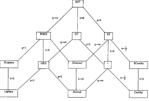
Many distributions can be considered in the generalized IV estimation procedure outlined in the previous section. The use of such distributions as the normal or Laplace will not model distributions that are both thick-tailed and asymmetric, both of which are often observed with economic and financial data. The skewed generalizedt, the exponential generalized beta of the second kind, and inverse hyperbolic sine distributions involve a small number of distributional parameters and permit modeling a wider range of data characteristics than the normal, Laplace,t, and many other common distributions. These distributions will be defined with basic properties and special cases summarized. We note that there are many other flexible families of distribu-tions that can be considered. Examples include the stable dis-tributions, the generalized hyperbolic distribution, and mixture distributions, to name a few. We chose to focus on our particular set of distributions because they involve few distributional para-meters and are relatively simple to implement while containing as special cases many of the common distributions employed in practice. Of course, there are a variety of reasons for which one may prefer to use a different parametric family, and the main re-sults of the article will continue to hold regardless of the family considered.
3.1 Skewed Generalizedt-Distribution (SGT)
The skewed generalizedt-distribution (SGT) was obtained by Theodossiou (1998) and can be defined by
SGT(y;m, λ, φ,p,q)
=p/
2φq1/pB(1/p,q)
×
1+ |y−m|p/(1+λsign(y−m))pqφpq+1/p,
whereB(·,·)is the beta function,mis the mode ofy, and the parametersp andq control the height and tails of the density.
The parameterφis a scale parameter andλdetermines the de-gree of skewness with the area to the left of the mode equal to
(1−λ)/2; thus, positive (negative) values forλcorrespond to positive (negative) skewness. Settingλ=0 in the SGT yields the generalizedt(GT) of McDonald and Newey (1988). Simi-larly, settingp=2 yields the skewedt(ST) of Hansen (1994), which includes the Student-tdistribution ifλ=0. The skewedt also includes the skewed Cauchy ifpq=1. Standardized values for skewness and kurtosis in the ranges(−∞,∞)and(1.8,∞), respectively, can be modeled with the SGT. The SGT has all moments of order less than the degrees of freedom (pq).
Another important class of flexible density functions corre-sponds to a limiting case of the SGT. When the parameter q grows indefinitely large, we obtain the skewed generalized er-ror distribution (SGED) defined by
SGED(y;m, λ, φ,p)=pe
−(|y−m|p/((1+λsign(y−m))pφp))
[2φŴ(1/p)] .
The parameterp in the SGED controls the height and tails of the density and λ controls the skewness. The SGED is sym-metric forλ=0 and positively (negatively) skewed for positive (negative) values ofλ. The symmetric SGED is also known as the generalized power (Subbotin1923) distribution. The SGED can easily be seen to include the skewed (λ=0)or symmet-ric(λ=0)Laplace (SLaplace or Laplace, respectively) when p=1 and the skewed(λ=0) or symmetric (λ=0)normal (SNormal or Normal, respectively) whenp=2. The interrela-tionships between the SGT and many of its special cases can be visualized as in Figure1.
3.2 Exponential Generalized Beta of the Second Kind (EGB2)
The four parameter EGB2 distribution is defined by the prob-ability density function
EGB2(y;m, φ,p,q)= e
p(y−m)/φ
[φB(p,q)(1+e(y−m)/φ)p+q], where the parametersφ,p, andqare assumed to be positive, cf. McDonald and Xu (1995);mandφare, respectively, location and scale parameters. The parametersp andqare shape para-meters. The EGB2 pdf is symmetric if and only ifpandqare
Figure 1. SGT distribution tree.
equal. The normal distribution is a limiting case of the EGB2 where the parametersp andq are equal and grow indefinitely large. Other special or limiting cases of the EGB2 include the Gumbel, Burr 2, generalized Gompertz, extreme value, and lo-gistic distributions. Standardized values for kurtosis are limited to the range (3.0, 9.0), and the standardized skewness coeffi-cient can assume values in the range (−2.0, 2.0).
3.3 Inverse Hyperbolic Sine (IHS)
The hyperbolic sine pdf was proposed by Johnson (1949) and allows for modeling a wide range of skewness and kur-tosis. The parameterization used here is slightly different than the one used by Johnson and is based on the transformation y=a+bsinh(λ+z/k)=a+bw where sinh is the hyper-bolic sign,zis a standard normal, anda,b,λ, andkare scaling constants related, respectively, to the mean (μ), variance (σ2), skewness, and kurtosis of the random variabley. The pdf ofy can be written as tive (negative) values of λ generate positive (negative) skew-ness, and zero corresponds to symmetry. Smaller values of k result in more leptokurtic distributions with the normal corre-sponding to the limiting case ofk→ ∞withλ=0. The IHS al-lows skewness and kurtosis in the range(3,∞)and(−∞,∞), respectively.
4. LARGE SAMPLE PROPERTIES
In this section we give an account of the asymptotic theory of the estimator. To keep things relatively simple we restrict
ρ(ε, γ ) to be smooth in γ, although the nonsmooth case can be considered, as in McDonald and Newey (1988). The first condition imposes the model of Equation (1) and identification.
Assumption 1. (a) Equation (1) is satisfied,Wi=(yi,Xi,Zi)
(i=1, . . . ,n) are iid, Xi1≡1, and Zi1≡1; (b) there is γ∗
such that γ˜ =γ∗+Op(1/√n); (c) there is a unique solution
α∗toE[ρ(εi−α, γ∗)] =0; (d) there is at most one solution to E[Ziρ(yi−Xi′β, γ∗)] =0.
The next condition imposes smoothness and dominance con-ditions.
Assumption 2. Bis compact,ρ(ε, γ )is continuously differ-entiable inεandγ, and there is a functiond(w)suchE[d(Wi)]
The final condition imposes rank conditions for asymptotic normality.
Assumption 3. Q=E[ZiZi′]is nonsingular, andG=E[Zi× X′i∂ρ(εi−α∗, γ∗)/∂ε]has rankp.
It is worth noting that the conditions imposed in Assump-tions1 through3 place our theoretical results in the conven-tional asymptotic framework. In particular, the full rank con-dition in Assumption3 rules out weak identification, and we assume a fixed number of instruments, and thus are not consid-ering many instrument asymptotic sequences. While consider-ing inference issues for the NLIV estimator under these condi-tions is an interesting question, we focus in this article on the potential efficiency gains that may be achieved by considering NLIV. We note that due to the GMM formulation of the prob-lem, the approaches to weak-identification robust inference of, for example, Stock and Wright (2000) and Kleibergen (2005) can readily be adopted. In many instrument settings, one can also consider the GMM approach of Newey and Windmeijer (2007).
It is also important to note that the model assumes indepen-dence between the structural errors and the instruments, rul-ing out heteroscedasticity. In principle, it will be simple to ac-commodate parametric forms of heteroscedasticity by suitably modifying the family of distributions to allow its parameters to depend on the instruments and then suitably modifying the moment conditions. However, the NLIV estimator will likely be inconsistent as formulated in the presence of heteroscedas-ticity. As such, researchers may wish to test for the presence of heteroscedasticity in the LIML or 2SLS residuals obtained in the first stage estimation, which can be done using any stan-dard test for heteroscedasticity. A particularly simple test that is available is a Hausman test of the difference between the NLIV and 2SLS or LIML estimates of the structural parameters. Un-der the assumption that the conditions given below such that NLIV attains the efficiency bound hold, this test can be per-formed simply by taking a quadratic form in the difference in estimated coefficients with the difference in estimated variances as the weighting matrix. We consider this in the empirical ex-amples in Section5.
To describe the asymptotic variance of the slope coefficients letσ2=E[ρ(εi−α∗, γ∗)2]. The asymptotic variance ofSβˆwill be
V=σ2S(G′Q−1G)−1S′.
The following result shows the consistency and asymptotic nor-mality of the slope coefficient estimatorSβˆ.
Theorem 1. If Assumptions1through3are satisfied then
√
nS(βˆ−β0)
d
−→N(0,V), Vˆ −→p V.
We now turn to the efficiency of the slope estimators. We motivated the estimator by analogy with the exogenousXcase, but it is not clear a priori what the efficiency properties of such an estimator might be. In particular, the form of the estimator seems to use only information about the marginal distribution of
ε, and one may wonder whether more information is available. We analyze efficiency in the semiparametric model where the only substantive assumption imposed is the independence ofz andε. This is a “limited information” semiparametric model, where no restrictions are placed on the conditional distribution of the endogenous regressors given the instrumentszand the
disturbanceε. This model also does not restrict the form of the distribution ofεor the other random variables.
We derive the efficiency bound without a full statement of regularity conditions to avoid much additional notation and clutter. This corresponds to a “formal” derivation, as is com-mon in the semiparametric efficiency literature, e.g., see Newey (1990). To state the efficiency result letxdenote the noncon-stant elements ofX, so that X=(1,x′)′. Letρ0(ε)denote the
location score forε, that isρ0(ε)=∂lnf0(ε)/∂ε, wheref0(ε)
is the marginal pdf ofε, let(ε,z)=E[x|ε,z], andε(ε,z)=
∂(ε,z)/∂ε. The following result is based on equation (23) of Newey (1990) and further calculations.
Theorem 2. In the semiparametric model of Equation (1) the semiparametric variance bound forSβisV∗=(E[s∗s∗′])−1
where
s∗= −ρ0(ε)(ε,z)−E[(ε,z)|ε]
−ε(ε,z)+E[ε(ε,z)|ε]. Ifx=π(z)+η, and(ε, η)is independent ofz, then
s∗= −ρ0(ε)π(z)−E[π(z)],
V∗=
E[ρ0(ε)2]− 1
var(π(z))−1.
Furthermore, forπ=π(z)andπ¯=E[π]we have, V=σ2E[∂lnf(ε−α∗, γ∗)/∂α]−2
×
E[(π− ¯π )Z′]Q−1E[Z(π− ¯π )′]2.
Finally, ifπ(z)is linear inZand the pdff0(ε)ofεialso satisfies f0(ε)=f(ε−α∗|γ∗)thenSβˆis an efficient estimator.
The semiparametric bound is the inverse of the variance of the efficient scores∗. It is interesting to note thats∗ depends only the scoreρ0(ε)for εand the conditional meanE[x|ε,Z].
When there is an additively separable, reduced-formπ(z)+η
for x the efficient score takes a more familiar form. In that case s∗ is analogous to the efficient score in a linear model with exogenous regressors, where the regressors are replaced by the reduced-form variablesπ(z). In particular, when the dis-turbance is Gaussian, the bound corresponds to the variance of an efficient instrumental variables estimator. More generally, it corresponds to a GMM estimator where the location score for the disturbance appears in place of the disturbance itself.
We also find that when the reduced form is additive, the as-ymptotic variance of the NLIV estimator depends only on the scalar function
E[ρ(εi−α∗, γ∗)2]/E[∂ρ(εi−α∗, γ∗)/∂ε]2,
and can be minimized by choosing α∗ and γ∗ to minimize that function. Also, the NLIV estimator will attain the semi-parametric variance bound when the reduced form is linear in Z, additive in an independent error, and the parametric family f(ε−α|γ )includes the truth atα∗andγ∗. That is, among all estimators that are consistent, asymptotically normal, and sat-isfy appropriate regularity conditions under the semiparametric model of Equation (1), the estimator we consider will be ef-ficient under the aforementioned conditions. This kind of effi-ciency property is sometimes termed “local effieffi-ciency,” refer-ring to the efficiency of the estimator over a subset of the whole semiparametric model.
When(ε,z)is not additive inzandε, attaining efficiency will require an approach different than NLIV based on flexible families of distributions. We focus here on NLIV because it is relatively simple and parsimonious and seems likely to capture much of the efficiency gain available from non-Gaussian distur-bances.
5. APPLICATIONS
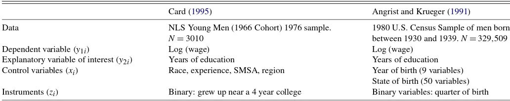
In this section we apply the NLIV estimators described in Section 2 to two models previously discussed in the litera-ture. The first application is to the problem considered by Card (1995), which uses 1976 wage and schooling data from the 1966 cohort from the NLS to estimate returns to schooling. The second example uses the model outlined by Angrist and Krueger (1991) with quarter of birth as instrumental variables to estimate returns to schooling based on the 1980 census for men born between 1930 and 1939. Table1summarizes each of these models and related datasets.
In each of the applications, we estimate models of the form
y1i=β0+β1y2i+γ1′xi+ε1i, y2i=π1′xi+π2′zi+η2i,
where y1i,y2i,xi, andzi, respectively, denote observations on the dependent variable, the explanatory variable of interest, a K1×1 vector of covariates, and aK2×1 vector of instrumental
variables withγ1, π1, andπ2 being conformable column
vec-tors of structural and reduced form parameters andε1iandη2i denoting structural and reduced form random disturbances.
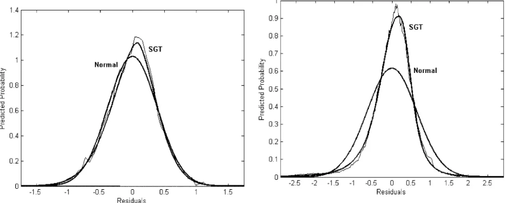
We start by estimating the parameters of the structural equation using ordinary least squares (OLS), limited informa-tion maximum likelihood (LIML), and two-stage least squares (2SLS) for the two examples and report the estimated schooling coefficients in Table2. Figures2and3depict the estimated dis-tributions of the first-step LIML residuals for the two examples
Table 1. Model summary
Card (1995) Angrist and Krueger (1991)
Data NLS Young Men (1966 Cohort) 1976 sample.
N=3010
1980 U.S. Census Sample of men born between 1930 and 1939.N=329,509
Dependent variable(y1i) Log (wage) Log (wage)
Explanatory variable of interest(y2i) Years of education Years of education
Control variables(xi) Race, experience, SMSA, region Year of birth (9 variables)
State of birth (50 variables) Instruments(zi) Binary: grew up near a 4 year college Binary variables: quarter of birth
Table 2. Estimation results of schooling coefficient
Card Angrist–Krueger homoscedastic Angrist–Krueger heteroscedastic
Estimator βˆ1 sβˆ
1 H βˆ1 sβˆ1 H βˆ1 sβˆ1 H
OLS 0.075 0.0035 0.067 0.0004 0.067 0.0004
LIML 0.132 0.0550 0.150 0.109 0.0198 0.419 0.109 0.0198 0.419
2SLS 0.132 0.0550 0.150 0.108 0.0195 0.418 0.108 0.0195 0.418
t 0.131 0.0508 0.149 0.078 0.0143 0.227 0.082 0.0144 0.239
GT 0.130 0.0504 0.152 0.081 0.0137 0.228 0.084 0.0138 0.236
EGB2 0.132 0.0521 0.149 0.070 0.0142 0.229 0.110 0.0156 0.229
IHS 0.132 0.0522 0.149 0.071∗ 0.0139∗ 0.224 0.111∗ 0.0151∗ 0.224
ST 0.128∗ 0.0502∗ 0.148 0.074 0.0144 0.225 0.112 0.0148 0.226
SGT 0.124 0.0582 0.149 0.075 0.0139 0.226 0.111 0.0140 0.227
μ2 13.3 108.1
NOTE: Estimated schooling coefficient and standard error using various estimators for Card (1995) and Angrist and Krueger (1991) examples summarized in Table1. The first two rows correspond to OLS and LIML, and the remaining rows give results using NLIV estimators corresponding to the specified distribution. Note that NLIV based on the normal is equivalent to 2SLS. The column labeledHreportsnHwhereHis the model selection criterion defined in the text.∗denotes the model chosen by the simple model selection procedure.
along with the normal distribution and SGT distribution implied by the maximum likelihood estimates of their respective para-meters. The Card residual distribution is much more similar to a normal than is the residual distribution for the Angrist–Krueger data, though the SGT provides an improved fit in both cases.
We also report the two-step NLIV estimates ofβ1based on
thet, GT, EGB2, IHS, ST, and SGT pdf’s with first step esti-mated by LIML in Table2. In both examples, we report results based on NLIV imposing homoscedasticity on the error terms. We also report results based on NLIV where we allow for het-eroscedasticity, specifically by allowing all distributional para-meters to be different depending on an individual’s quarter of birth, for the Angrist–Krueger example; these estimates are re-ported in the column labeled “Angrist–Krueger heteroscedastic-ity.” Also of interest is the value of the concentration parameter
μ2=(π2′Z′(I−X(X′X)−1X′)Zπ2/Var(η2i)), which provides a measure of the strength of the instruments. It takes on a rather small value, 13, in the Card data and is large, 108, in the Angrist and Krueger data. In all cases, we report only results for the co-efficient on the endogenous variable as this is the parameter of
Figure 2. LIML residual distribution from Card data.
interest in these studies. While there is obviously some varia-tion, the same basic results hold for the other covariates in each model which generally exhibit efficiency gains that are similar to those for the coefficient on the endogenous variable.
Looking at the results, we see that the NLIV estimates agree fairly closely with the LIML estimates in the Card example, but are quite different in the Angrist–Krueger example when ho-moscedasticity is imposed. This difference is essentially elim-inated when we allow for heteroscedasticity. In the Card ex-ample the NLIV standard errors are quite close to the 2SLS standard errors. Given that the NLIV asymptotic approxima-tion works relatively poorly with low concentraapproxima-tion parameter in the simulation study reported below, we find no evidence of improvement in the Card example. In the Angrist–Krueger ex-ample, where the concentration parameter is quite high, we find evidence of substantial efficiency gains of about 30%. In the Card example, we find the model selection procedure chooses the ST, which gives an estimate of the returns to schooling of 0.128 with an estimated standard error of 0.0502; in this exam-ple, the LIML estimate is 0.132 with standard error of 0.0550.
Figure 3. LIML residual distribution from Angrist and Krueger data.
In the Angrist–Krueger example, the model selection procedure chooses the IHS, which produces an estimate of 0.071 with standard error of 0.0139 in the homoscedastic case and 0.111 with standard error of 0.0151 in the heteroscedastic case while the LIML estimate is 0.109 with standard error 0.0198. Finally, we can compare the estimated schooling coefficient from LIML (or 2SLS) to the NLIV estimate to test for heteroscedasticity (and potentially other types of misspecification). Under the as-sumption that the conditions required for the NLIV estimator to attain the efficiency bound are satisfied, the standard error of this difference coefficients is simply given as the square root of the difference in the estimated variances, and the difference between the coefficients divided by this standard error will be asymptotically standard normal. For the Card example, we ob-tain a value of this test statistic of 0.178 using LIML and the ST results and will thus fail to reject the hypothesis of homoscedas-ticity at conventional levels. On the other hand, the value of this statistic is 2.62 using LIML and the IHS results in the Angrist– Krueger example under homoscedasticity, and we will reject the hypothesis of independence at usual levels. However, in the het-eroscedastic specification, we obtain a test statistic of−0.156 and will fail to reject the hypothesis at conventional levels.
6. SIMULATION RESULTS
We investigate the properties of some NLIV estimators using Monte Carlo simulations that are similar to the data generating process considered in Newey and Windmeijer (2007). Let the structural relation of interest be
y1i=y2iβ+εi,
with the corresponding reduced form representation ofy2ibeing
y2i=z′iπ+η2i,
where the structural disturbance is written in terms of reduced form disturbances as follows:
εi=ρη2i+
1−ρ2η 1i.
To complete the data generating process for the Monte Carlo study observations of the exogenous variables (instruments) will be generated as pends upon the values of the concentration parameter (μ2), the number of instruments (K), the correlation(ρ)between the structural and reduced form (fory2i) disturbances, the
distrib-ution of the disturbances, and the sample size. In the sample design we generate samples of size 200 with β =0.1, μ2=
15,30,60, K =3 or 10, and ρ =0.3 or 0.5. We consider three different distributions forη1iandη2i: (1) standard normal;
(2) mixture of normal variables or a variance-contaminated nor-mal,U∗N[0,1/9] +(1−U)∗N[0,9]whereUis an independent Bernoulli(0.9)random variable; and (3) lognormal. In order for each error distribution to have a zero mean and unitary vari-ance the third reduced form error distribution is generated as
(eN√[0,1]−e0.5
e(e−1) ).
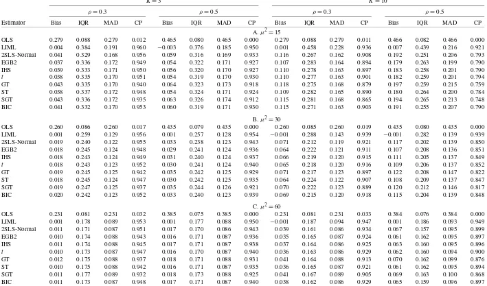
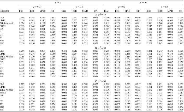
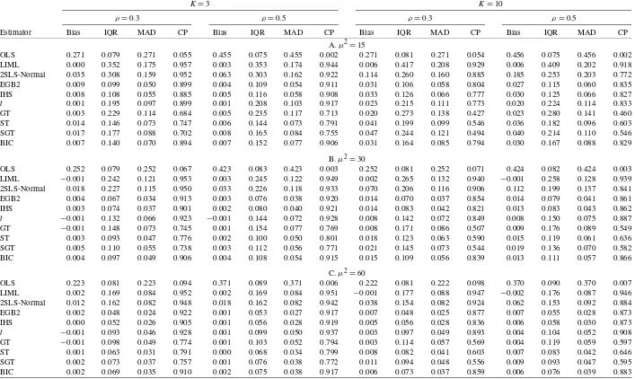
Monte Carlo simulation results of the alternative estimators of the structural slope coefficient (β=0.1)based on 20,000 simulation replications are summarized in Tables3,4, and5. We report median bias (Bias), interquartile range (IQR), me-dian absolute deviation (MAD), and 95% confidence interval coverage probability (CP) for estimates ofβ obtained by OLS, 2SLS, and LIML, as well as the two-step NLIV estimators ofβ
corresponding to thet, GT, EGB2, IHS, ST, and SGT pdf’s us-ing LIML first step estimates and QMLE based on the LIML residuals to obtain estimates of the distributional parameters.
Results for the normal error distribution are summarized in Table3. In this case, the median sample bias is minimized by LIML among the estimators we consider. Among the NLIV es-timators, the bias and spread as measured by the interquartile range are largely insensitive to the pdf. In this case, the NLIV estimators all perform worse than LIML in terms of median bias, but appear to have considerably less dispersion as mea-sured by IQR. NLIV estimators also dominate LIML in terms of estimator risk as measured by MAD. We note that 2SLS, which is numerically identical to NLIV using a normal distri-bution, does slightly better than the other NLIV estimators. As expected, we see that coverage probabilities for NLIV estima-tors may be distorted when instruments are weak(μ2=15)or many (K=10) and that this distortion decreases as μ2/K in-creases.
The results corresponding to the case of a mixed normal or variance contaminated error distribution that is symmetric with thick tails (standardized kurtosis is approximately 20) are re-ported in Table4. The median bias of all estimators decreases asμ2/Kincreases. The NLIV estimators produce substantially smaller values of IQR than LIML or 2SLS with IQR’s less than 50% those of LIML or 2SLS in some cases. The gains are also apparent in MAD terms where improvements are sim-ilar to those in IQR. It is interesting that in this case, unlike the normal design, the majority of NLIV estimators have median biases that are comparable to LIML. The NLIV estimators, es-pecially those based on the SGT, do suffer somewhat relative to LIML in terms of coverage probability. We also see that us-ing the simple model selection procedure produces an estimator with quite favorable properties.
The impact of a skewed and leptokurtic error distribution on estimator performance can be seen in Table5. As in the thick-tailed case above, we see that the NLIV estimators show large improvements in efficiency that are not necessarily accompa-nied by large increases in bias relative to LIML or 2SLS. Not surprisingly, the NLIV estimators based on possibly skewed pdf’s show the greatest improvement with the exception of the SGT, which may need a larger sample size to accurately model the underlying error distribution. As before, we see that the NLIV estimators suffer somewhat in terms of coverage relative to LIML. This is especially true for the SGT and GT, which perform very poorly. We also see that model selection proce-dure produces an estimator that performs well overall.
Jour
nal
of
Business
&
Economic
Statistics
,
J
an
uar
y
2010
Table 3. Simulation results from normal design
K=3 K=10
ρ=0.3 ρ=0.5 ρ=0.3 ρ=0.5
Estimator Bias IQR MAD CP Bias IQR MAD CP Bias IQR MAD CP Bias IQR MAD CP
A.μ2=15
OLS 0.279 0.088 0.279 0.012 0.465 0.080 0.465 0.000 0.279 0.088 0.279 0.011 0.466 0.082 0.466 0.000 LIML 0.004 0.384 0.191 0.960 −0.003 0.376 0.185 0.950 0.001 0.458 0.228 0.936 0.007 0.439 0.216 0.921 2SLS-Normal 0.041 0.329 0.168 0.956 0.059 0.316 0.169 0.933 0.116 0.267 0.162 0.908 0.192 0.251 0.206 0.793 EGB2 0.037 0.336 0.172 0.949 0.054 0.322 0.171 0.927 0.107 0.283 0.164 0.894 0.179 0.263 0.199 0.790 IHS 0.039 0.333 0.171 0.950 0.056 0.320 0.170 0.927 0.110 0.278 0.163 0.897 0.183 0.258 0.201 0.790
t 0.038 0.335 0.170 0.951 0.054 0.319 0.170 0.930 0.110 0.277 0.163 0.901 0.182 0.259 0.201 0.794
GT 0.043 0.335 0.170 0.940 0.064 0.323 0.173 0.918 0.118 0.275 0.168 0.879 0.197 0.259 0.215 0.759 ST 0.038 0.337 0.172 0.948 0.054 0.324 0.171 0.924 0.109 0.282 0.165 0.890 0.180 0.264 0.200 0.784 SGT 0.043 0.336 0.172 0.935 0.063 0.326 0.174 0.912 0.115 0.281 0.168 0.865 0.194 0.265 0.213 0.748 BIC 0.041 0.332 0.170 0.953 0.060 0.319 0.171 0.930 0.115 0.271 0.163 0.903 0.191 0.255 0.207 0.790
B.μ2=30
OLS 0.260 0.086 0.260 0.017 0.435 0.079 0.435 0.000 0.260 0.085 0.260 0.019 0.435 0.080 0.435 0.000 LIML 0.001 0.259 0.129 0.956 0.001 0.257 0.128 0.954 −0.001 0.288 0.143 0.939 −0.001 0.282 0.139 0.939 2SLS-Normal 0.019 0.240 0.122 0.955 0.033 0.238 0.123 0.943 0.071 0.212 0.119 0.921 0.117 0.202 0.139 0.850 EGB2 0.018 0.245 0.124 0.948 0.029 0.241 0.124 0.936 0.064 0.222 0.121 0.911 0.107 0.208 0.136 0.851 IHS 0.018 0.243 0.124 0.949 0.031 0.240 0.124 0.937 0.066 0.219 0.120 0.915 0.111 0.205 0.137 0.849
t 0.018 0.243 0.123 0.952 0.030 0.241 0.124 0.940 0.065 0.218 0.120 0.916 0.109 0.206 0.137 0.852
GT 0.019 0.245 0.125 0.942 0.035 0.242 0.125 0.929 0.071 0.217 0.123 0.897 0.122 0.208 0.147 0.822 ST 0.018 0.245 0.124 0.947 0.030 0.242 0.125 0.935 0.064 0.224 0.122 0.907 0.108 0.209 0.137 0.847 SGT 0.019 0.247 0.125 0.937 0.035 0.244 0.126 0.921 0.070 0.222 0.123 0.889 0.120 0.212 0.146 0.817 BIC 0.020 0.242 0.123 0.952 0.033 0.240 0.123 0.939 0.069 0.215 0.120 0.918 0.115 0.204 0.139 0.848
C.μ2=60
OLS 0.231 0.081 0.231 0.032 0.385 0.075 0.385 0.000 0.231 0.081 0.231 0.033 0.384 0.076 0.384 0.000 LIML 0.001 0.178 0.089 0.953 0.001 0.177 0.088 0.950 −0.001 0.187 0.094 0.947 0.001 0.186 0.093 0.949 2SLS-Normal 0.011 0.171 0.087 0.951 0.017 0.170 0.086 0.943 0.039 0.161 0.086 0.934 0.067 0.157 0.095 0.899 EGB2 0.010 0.174 0.088 0.943 0.016 0.171 0.087 0.936 0.035 0.165 0.087 0.924 0.061 0.162 0.095 0.897 IHS 0.011 0.174 0.088 0.945 0.017 0.171 0.087 0.938 0.037 0.164 0.086 0.925 0.063 0.160 0.095 0.896
t 0.010 0.173 0.087 0.947 0.016 0.170 0.087 0.940 0.036 0.163 0.086 0.929 0.062 0.160 0.094 0.900
GT 0.012 0.175 0.088 0.937 0.018 0.171 0.088 0.931 0.041 0.164 0.088 0.913 0.070 0.162 0.099 0.876 ST 0.010 0.175 0.088 0.942 0.016 0.171 0.087 0.935 0.036 0.165 0.087 0.921 0.061 0.162 0.095 0.894 SGT 0.011 0.177 0.089 0.932 0.018 0.173 0.088 0.925 0.041 0.167 0.089 0.905 0.069 0.163 0.100 0.868 BIC 0.011 0.173 0.087 0.948 0.017 0.171 0.087 0.940 0.038 0.162 0.086 0.929 0.065 0.159 0.096 0.897 NOTE: Results for normal simulation model described in text. The design uses 200 observations, and all results are based on 20,000 simulation replications. We report median bias (Bias), interquartile range (IQR), median absolute deviation (MAD), and 95% confidence interval coverage (CP). Rows labeled EGB2, IHS,t, GT, ST, and SGT correspond to NLIV estimates based on the distribution given in the row label. At each iteration, BIC uses the estimator selected by the model selection procedure outlined in the text. We also note that 2SLS corresponds to NLIV when the assumed error distribution is normal.
McDonald,
and
Ne
w
e
y:
Instr
umental
V
ar
iab
les
E
stimation
W
ith
F
le
xib
le
D
istr
ib
utions
21
Table 4. Simulation results from normal mixture design
K=3 K=10
ρ=0.3 ρ=0.5 ρ=0.3 ρ=0.5
Estimator Bias IQR MAD CP Bias IQR MAD CP Bias IQR MAD CP Bias IQR MAD CP
A.μ2=15
OLS 0.278 0.244 0.279 0.192 0.464 0.227 0.464 0.025 0.280 0.248 0.281 0.186 0.464 0.225 0.464 0.026 LIML 0.000 0.362 0.180 0.958 0.002 0.357 0.177 0.953 0.004 0.435 0.217 0.933 0.005 0.410 0.201 0.925 2SLS-Normal 0.036 0.315 0.162 0.952 0.059 0.307 0.164 0.932 0.112 0.279 0.163 0.881 0.186 0.260 0.203 0.780 EGB2 0.002 0.146 0.073 0.924 0.002 0.145 0.072 0.929 0.006 0.160 0.080 0.861 0.013 0.153 0.077 0.874 IHS 0.002 0.163 0.081 0.904 0.001 0.162 0.081 0.911 0.007 0.191 0.096 0.794 0.011 0.185 0.094 0.799
t 0.001 0.145 0.073 0.918 −0.001 0.146 0.073 0.923 0.003 0.166 0.083 0.831 0.006 0.161 0.081 0.844
GT 0.001 0.164 0.082 0.830 0.002 0.164 0.082 0.831 0.010 0.194 0.098 0.655 0.016 0.184 0.094 0.667 ST 0.001 0.147 0.073 0.912 0.000 0.148 0.074 0.917 0.003 0.169 0.085 0.821 0.007 0.163 0.082 0.835 SGT 0.000 0.168 0.084 0.816 0.002 0.166 0.083 0.819 0.009 0.199 0.100 0.639 0.014 0.190 0.097 0.647 BIC 0.000 0.150 0.075 0.918 0.000 0.151 0.075 0.923 0.005 0.172 0.086 0.839 0.009 0.167 0.084 0.845
B.μ2=30
OLS 0.259 0.225 0.260 0.195 0.432 0.212 0.432 0.028 0.258 0.234 0.259 0.208 0.431 0.213 0.431 0.028 LIML −0.001 0.246 0.123 0.960 0.002 0.244 0.121 0.954 −0.001 0.278 0.138 0.942 0.001 0.271 0.134 0.939 2SLS-Normal 0.018 0.230 0.116 0.956 0.032 0.227 0.117 0.939 0.067 0.215 0.119 0.910 0.114 0.210 0.138 0.842 EGB2 0.001 0.103 0.052 0.933 0.001 0.101 0.050 0.934 0.003 0.108 0.054 0.894 0.005 0.106 0.053 0.903 IHS 0.001 0.113 0.057 0.915 0.000 0.112 0.056 0.920 0.002 0.124 0.062 0.853 0.004 0.123 0.062 0.852
t 0.000 0.103 0.051 0.925 −0.001 0.100 0.050 0.929 0.000 0.110 0.055 0.881 0.002 0.108 0.054 0.886
GT 0.000 0.111 0.056 0.852 0.000 0.111 0.055 0.855 0.002 0.125 0.063 0.723 0.004 0.125 0.062 0.730 ST 0.000 0.103 0.051 0.921 −0.001 0.101 0.051 0.926 0.000 0.111 0.055 0.870 0.002 0.108 0.054 0.876 SGT 0.000 0.115 0.057 0.838 0.000 0.114 0.057 0.845 0.002 0.128 0.064 0.709 0.005 0.127 0.064 0.714 BIC 0.000 0.105 0.053 0.928 −0.001 0.103 0.052 0.931 0.002 0.113 0.056 0.879 0.002 0.112 0.056 0.885
C.μ2=60
OLS 0.227 0.207 0.228 0.220 0.380 0.193 0.380 0.033 0.228 0.206 0.229 0.217 0.378 0.191 0.378 0.033 LIML 0.001 0.172 0.086 0.955 −0.001 0.175 0.088 0.949 0.000 0.178 0.089 0.945 −0.001 0.179 0.089 0.947 2SLS-Normal 0.009 0.166 0.084 0.952 0.015 0.169 0.085 0.941 0.039 0.157 0.084 0.925 0.062 0.156 0.092 0.888 EGB2 0.001 0.071 0.036 0.934 0.001 0.071 0.036 0.936 0.002 0.074 0.037 0.914 0.002 0.073 0.037 0.911 IHS 0.000 0.078 0.039 0.922 0.001 0.078 0.039 0.924 0.002 0.084 0.042 0.877 0.002 0.085 0.043 0.873
t 0.000 0.070 0.035 0.931 0.000 0.071 0.035 0.934 0.001 0.075 0.037 0.902 0.001 0.075 0.037 0.901
GT 0.000 0.076 0.038 0.869 0.000 0.077 0.038 0.871 0.002 0.084 0.042 0.772 0.002 0.084 0.042 0.769 ST 0.000 0.071 0.036 0.926 0.000 0.071 0.036 0.929 0.001 0.075 0.037 0.892 0.000 0.075 0.038 0.892 SGT 0.000 0.077 0.039 0.860 0.001 0.078 0.039 0.862 0.002 0.085 0.043 0.753 0.002 0.086 0.043 0.754 BIC 0.000 0.072 0.036 0.931 0.001 0.072 0.036 0.934 0.002 0.077 0.038 0.902 0.000 0.076 0.038 0.898 NOTE: Results for normal mixture simulation model described in text. The design uses 200 observations, and all results are based on 20,000 simulation replications. We report median bias (Bias), interquartile range (IQR), median absolute deviation (MAD), and 95% confidence interval coverage (CP). Rows labeled EGB2, IHS,t, GT, ST, and SGT correspond to NLIV estimates based on the distribution given in the row label. At each iteration, BIC uses the estimator selected by the model selection procedure outlined in the text. We also note that 2SLS corresponds to NLIV when the assumed error distribution is normal.
Jour
nal
of
Business
&
Economic
Statistics
,
J
an
uar
y
2010
Table 5. Simulation results from lognormal design
K=3 K=10
ρ=0.3 ρ=0.5 ρ=0.3 ρ=0.5
Estimator Bias IQR MAD CP Bias IQR MAD CP Bias IQR MAD CP Bias IQR MAD CP
A.μ2=15
OLS 0.271 0.079 0.271 0.055 0.455 0.075 0.455 0.002 0.271 0.081 0.271 0.054 0.456 0.075 0.456 0.002 LIML 0.000 0.352 0.175 0.957 0.003 0.353 0.174 0.944 0.006 0.417 0.208 0.929 0.006 0.409 0.202 0.918 2SLS-Normal 0.035 0.308 0.159 0.952 0.063 0.303 0.162 0.922 0.114 0.260 0.160 0.885 0.185 0.253 0.203 0.772 EGB2 0.009 0.099 0.050 0.899 0.004 0.109 0.054 0.911 0.031 0.106 0.058 0.804 0.027 0.115 0.060 0.835 IHS 0.008 0.108 0.055 0.885 0.005 0.116 0.058 0.908 0.033 0.126 0.066 0.777 0.030 0.125 0.066 0.827
t 0.001 0.195 0.097 0.899 0.001 0.208 0.103 0.917 0.023 0.215 0.111 0.773 0.020 0.224 0.114 0.833
GT 0.003 0.229 0.114 0.684 0.005 0.235 0.117 0.713 0.020 0.273 0.138 0.427 0.023 0.280 0.141 0.460 ST 0.014 0.146 0.073 0.747 0.006 0.144 0.073 0.791 0.041 0.199 0.099 0.546 0.036 0.182 0.096 0.603 SGT 0.017 0.177 0.088 0.702 0.008 0.165 0.084 0.755 0.047 0.244 0.121 0.494 0.040 0.214 0.110 0.546 BIC 0.007 0.140 0.070 0.894 0.007 0.152 0.077 0.906 0.031 0.164 0.085 0.794 0.030 0.167 0.088 0.829
B.μ2=30
OLS 0.252 0.079 0.252 0.067 0.423 0.083 0.423 0.003 0.252 0.081 0.252 0.071 0.424 0.082 0.424 0.003 LIML −0.001 0.242 0.121 0.953 0.003 0.245 0.122 0.949 0.002 0.265 0.132 0.940 −0.001 0.258 0.128 0.939 2SLS-Normal 0.018 0.227 0.115 0.950 0.033 0.226 0.118 0.933 0.070 0.206 0.116 0.906 0.112 0.199 0.137 0.841 EGB2 0.004 0.067 0.034 0.913 0.003 0.076 0.038 0.920 0.014 0.070 0.037 0.854 0.014 0.079 0.041 0.861 IHS 0.003 0.074 0.037 0.901 0.002 0.080 0.040 0.921 0.014 0.083 0.042 0.821 0.013 0.083 0.043 0.862
t −0.001 0.132 0.066 0.923 −0.001 0.144 0.072 0.928 0.008 0.142 0.072 0.849 0.008 0.150 0.075 0.887
GT −0.001 0.148 0.073 0.745 0.001 0.154 0.077 0.769 0.008 0.171 0.086 0.507 0.009 0.176 0.089 0.549 ST 0.003 0.093 0.047 0.776 0.002 0.100 0.050 0.801 0.018 0.123 0.063 0.590 0.015 0.119 0.061 0.636 SGT 0.005 0.110 0.055 0.738 0.003 0.112 0.056 0.771 0.021 0.145 0.073 0.544 0.019 0.136 0.070 0.582 BIC 0.004 0.097 0.049 0.906 0.004 0.108 0.054 0.915 0.015 0.109 0.056 0.839 0.013 0.111 0.057 0.866
C.μ2=60
OLS 0.223 0.081 0.223 0.094 0.371 0.089 0.371 0.006 0.222 0.081 0.222 0.098 0.370 0.090 0.370 0.007 LIML 0.002 0.169 0.084 0.952 0.002 0.169 0.084 0.951 −0.001 0.177 0.088 0.947 −0.002 0.176 0.087 0.946 2SLS-Normal 0.012 0.162 0.082 0.948 0.018 0.162 0.082 0.942 0.038 0.154 0.082 0.924 0.062 0.153 0.092 0.884 EGB2 0.002 0.048 0.024 0.922 0.001 0.053 0.027 0.917 0.007 0.048 0.025 0.877 0.007 0.055 0.028 0.873 IHS 0.000 0.052 0.026 0.905 0.001 0.056 0.028 0.919 0.005 0.056 0.028 0.836 0.006 0.058 0.030 0.873
t −0.001 0.093 0.046 0.928 0.001 0.099 0.050 0.937 0.003 0.097 0.049 0.893 0.004 0.104 0.052 0.908
GT −0.001 0.098 0.049 0.774 0.001 0.103 0.052 0.794 0.003 0.114 0.057 0.569 0.004 0.119 0.059 0.597 ST 0.001 0.063 0.031 0.791 0.000 0.068 0.034 0.799 0.008 0.082 0.041 0.603 0.007 0.083 0.042 0.646 SGT 0.002 0.073 0.037 0.757 0.001 0.076 0.038 0.772 0.011 0.094 0.048 0.556 0.009 0.093 0.047 0.595 BIC 0.002 0.069 0.035 0.910 0.002 0.075 0.038 0.917 0.006 0.073 0.037 0.859 0.006 0.076 0.039 0.883 NOTE: Results for lognormal simulation model described in text. The design uses 200 observations, and all results are based on 20,000 simulation replications. We report median bias (Bias), interquartile range (IQR), median absolute deviation (MAD), and 95% confidence interval coverage (CP). Rows labeled EGB2, IHS,t, GT, ST, and SGT correspond to NLIV estimates based on the distribution given in the row label. At each iteration, BIC uses the estimator selected by the model selection procedure outlined in the text. We also note that 2SLS corresponds to NLIV when the assumed error distribution is normal.
Overall, the simulation results are encouraging for the NLIV estimators. In the case of nonnormal disturbances, the NLIV estimators show substantial gains relative to LIML or 2SLS in terms of dispersion and MAD. These gains are accompanied by only minor losses in the case of normal errors. As expected, the coverage probabilities of interval estimates based on the NLIV estimators are somewhat distorted in cases of weak or many instruments, though this can likely be remedied by adopt-ing existadopt-ing results from the weak and many instruments litera-ture in these cases. There also appear to be some distortions in coverage probabilities even when the instruments are stronger, though they are generally minor. This can be the result of the small sample or may suggest that pursuing other approaches to estimating standard errors, such as the bootstrap, may be desir-able in this context.
7. SUMMARY AND CONCLUSIONS
In this article, we consider efficiency gains that may be avail-able using moment conditions which are nonlinear in the dis-turbances. The nonlinear functions we consider are based on the use of flexible parametric families of disturbance distribu-tions. We illustrate the approach in two empirical examples. In both examples, the NLIV estimators are associated with smaller standard errors than conventional IV estimators. Monte Carlo simulations demonstrate that while NLIV estimators may be as-sociated with modest efficiency loss in the case of normal error distributions, they offer the possibility of significant efficiency improvements in the presence of thick-tailed and/or skewed er-ror distributions. law of large numbers (LLN) and the continuous mapping the-orem (CMT). Let g(β)=E[Ziρ(yi−Xi′β, γ∗)] and Q(β)=
It follows as in the proof of theorem 2.6 of Newey and McFad-den (1994) that
sup β∈Bˆ
g(β)′Qˆ−1gˆ(β)/n−Q(β)−→p 0.
Also, the objective function Q(β) has a unique minimum at
β∗, so it follows as in the proof of theorem 2.6 of Newey and
first unit vector. It then follows by an expansion that
√
It also follows by standard GMM arguments that
√ By the Lindberg–Levy central limit theorem,
iZiρ(ui, γ∗)/
giving the first conclusion. The second conclusion also follows by a standard argument.
Proof of Theorem2
Here letδ denote the slope coefficientsSβ. By the assump-tion thatzandεare independent the joint pdf ofε,z, andXtake the form
f(ε)g(z)h(x|ε,z),
wheref andgdenote the marginal densities ofεandz, respec-tively, andhis the conditional pdf ofX givenzandε. Substi-tutingy−x′δ forεand differentiating, we find the score forδ
to be
sδ= −x{ρ0(ε)+∂lnh(x|ε,Z)∂ε},
ρ0(ε)=∂lnf0(ε)/∂ε.
Applying equation (23) of Newey (1990), the efficient score is
s∗=E[sβ|z, ε] −E[sβ|ε].
Note also that by interchanging the order of differentiation and integration we have
E[x∂lnh(x|ε,z) ∂ε|ε,z] =
x[∂h(x|ε,z)/∂ε]dx=ε(ε,z). Then applying iterated expectations gives the first conclusion.
Next, ifx=π(z)+ηforηindependent ofZwe have
Substituting these expressions in the formula fors∗ gives the second conclusion.
By the partitioned inverse formula it follows that
V=σ2S′(G′Q−1G)−1S=σ2/(E[ρεi])2(Q˜ +aa′−aa′/1)−1
=σ2/(E[ρεi])2Q˜−1, giving the third conclusion.
For the fourth conclusion, note that whenπi′is a linear com-bination ofZithen(0, πi′− ¯π′)is too, so that
E[(0, πi′− ¯π′)′Zi′]Q−1E[Zi(0, πi′− ¯π′)]
=E[(0, πi′− ¯π′)′(0, πi′− ¯π′)] =diag[0,var(πi)]. Furthermore, if f0(ε)=f(ε−α∗, γ∗)thenρ0(ε)=ρ(ε) and
the information matrix equality for a location parameter gives E[ρεi] = −σ2=E[ρ0(ε)2], so that
V=E[ρ0(ε)2]
var(πi)−1=(E[s∗s∗′])−1.
ACKNOWLEDGMENTS
The authors thank the outstanding research assistance pro-vided by Brigham Frandsen, Samuel Dastrup, and Randall Lewis. The authors also thank two anonymous referees and an editor for constructive comments that improved the article. All remaining errors are, of course, ours. This work was supported by NSF grants SES-0136869 and SES-0617836, funding from the William S. Fishman Faculty Research Fund and IBM Cor-poration Faculty Research Fund at the Graduate School of Busi-ness, the University of Chicago, and funding for the Clayne L. Pope Professorship at BYU.
[Received December 2006. Revised January 2008.]
REFERENCES
Andrews, D. W. K. (1999), “Consistent Moment Selection Procedures for Gen-eralized Method of Moments,”Econometrica, 67, 543–564. [15]
Angrist, J., and Krueger, A. K. (1991), “Does Compulsory School Attendance Affect Schooling and Earnings?”Quarterly Journal of Economics, 106, 979–1014. [13,17,18]
Card, D. (1995), “Using Geographic Variation in College Proximity to Estimate the Return to Schooling,” inAspects of Labour Market Behavior: Essays in Honour of John Vanderkamp, eds. L. N. Christophides, E. K. Grant, and R. Swidinsky, Toronto: University of Toronto Press, pp. 201–222. [13,17,
18]
Chernozhukov, V., and Hansen, C. (2005), “An IV Model of Quantile Treatment Effects,”Econometrica, 73, 245–261. [13]
Hansen, B. E. (1994), “Autoregressive Conditional Density Estimation,” Inter-national Economic Review, 35, 705–730. [15]
Hansen, C., McDonald, J. B., and Theodossiou, P. (2005), “Some Flexi-ble Parametric Models for Partially Adaptive Estimators of Econometric Models,” working paper. Available athttp:// www.economics-ejournal.org/ economics/ journalarticles/ 2007-7. [13,16]
Honore, B. E., and Hu, L. (2004), “On the Performance of Some Robust Instru-mental Variables Estimators,”Journal of Business & Economic Statistics, 22, 30–39. [13]
Johnson, N. L. (1949), “Systems of Frequency Curves Generated by Methods of Translation,”Biometrica, 36, 149–176. [16]
Kleibergen, F. (2005), “Testing Parameters in GMM Without Assuming That They Are Identified,”Econometrica, 73, 1103–1124. [16]
McDonald, J. B., and Newey, W. K. (1988), “Partially Adaptive Estimation of Regression Models via the GeneralizedtDistribution,”Econometric The-ory, 4, 428–457. [13,15]
McDonald, J. B., and White, S. B. (1993), “Comparison of Robust, Adaptive, and Partially Adaptive Estimators of Regression Models,”Econometric Re-views, 37, 273–278. [13]
McDonald, J. B., and Xu, Y. J. (1995), “A Generalization of the Beta Distribu-tion With ApplicaDistribu-tions,”Journal of Econometrics, 66, 133–152. Errata, 69 (1995), 427–428. [15]
Newey, W. K. (1988), “Adaptive Estimation of Regression Models via Moment Restrictions,”Journal of Econometrics, 38, 301–339. [16]
(1990), “Semiparametric Efficiency Bounds,” Journal of Applied Econometrics, 5, 99–135. [13,17,24]
Newey, W. K., and McFadden, D. (1994), “Large Sample Estimation and Hy-pothesis Testing,” inHandbook of Econometrics, Vol. 4, eds. R. Engle and D. McFadden, Amsterdam: North Holland, Chapter 36. [23]
Newey, W. K., and Windmeijer, F. (2007), “GMM With Many Weak Moment Conditions,” working paper, MIT. [16,19]
Stock, J. H., and Wright, J. H. (2000), “GMM With Weak Identification,”
Econometrica, 68, 1055–1096. [16]
Subbotin, M. T. (1923), “On the Law of Frequency of Error,”Mathematicheskii Sbornik, 31, 296–301. [15]
Theodossiou, P. (1998), “Financial Data and the Skewed Generalizedt Distrib-ution,”Management Science, 44, 1650–1661. [15]
White, H. (1982), “Maximum Likelihood Estimation of Misspecified Models,”
Econometrica, 50 (1), 1–25. [14]