Full Terms & Conditions of access and use can be found at
http://www.tandfonline.com/action/journalInformation?journalCode=ubes20
Download by: [Universitas Maritim Raja Ali Haji] Date: 11 January 2016, At: 19:13
Journal of Business & Economic Statistics
ISSN: 0735-0015 (Print) 1537-2707 (Online) Journal homepage: http://www.tandfonline.com/loi/ubes20
Comment
Lutz Kilian
To cite this article: Lutz Kilian (2015) Comment, Journal of Business & Economic Statistics, 33:1, 13-17, DOI: 10.1080/07350015.2014.969430
To link to this article: http://dx.doi.org/10.1080/07350015.2014.969430
Published online: 26 Jan 2015.
Submit your article to this journal
Article views: 130
View related articles
REFERENCES
Calhoun, G. (2011), “Out-of-Sample Comparisons of Overfit Models,” Working Paper 10002, Iowa State University. [12]
Clark, T. E., and McCracken, M. W. (2013), “Advances in Forecast Evaluation,” inHandbook of Economic Forecasting (Vol. 2), eds. G. Elliott and A. Timmermann, Amsterdam: Elsevier. [12]
——— (2014), “Nested Forecast Model Comparisons: A New Approach to Testing Equal Accuracy,”Journal of Econometrics, forthcoming. [12]
Diebold, F. X., and Mariano, R. S. (1995), “Comparing Predictive Ac-curacy,” Journal of Business and Economic Statistics, 13, 253–263. [12]
Giacomini, R., and White, H. (2006), “Tests of Conditional Predictive Ability,”
Econometrica, 74, 1545–1578. [12]
Harvey, D. I., Leybourne, S. J., and Newbold, P. (1997), “Testing the Equality of Prediction Mean Squared Errors,”International Journal of Forecasting, 13, 281–291. [12]
Comment
Lutz K
ILIANDepartment of Economics, University of Michigan, Ann Arbor, MI 48109 ([email protected])
Professor Diebold’s personal reflections about the history of the DM test remind us that this test was originally designed to compare the accuracy of model-free forecasts such as judgmen-tal forecasts generated by experts, forecasts implied by financial markets, survey forecasts, or forecasts based on prediction mar-kets. This test is used routinely in applied work. For example, Baumeister and Kilian (2012) use the DM test to compare oil price forecasts based on prices of oil futures contracts against the no-change forecast.
Much of the econometric literature that builds on Diebold and Mariano (1995), in contrast, has been preoccupied with testing the validity of predictive models in pseudo-out-of-sample envi-ronments. In this more recent literature, the concern actually is not the forecasting ability of the models in question. Rather the focus is on testing the null hypothesis that there is no predictive relationship from one variable to another in population. Testing for the existence of a predictive relationship in population is viewed as an indirect test of all economic models that suggest such a predictive relationship. A case in point is studies of the predictive power of monetary fundamentals for the exchange rate (e.g., Mark1995). Although this testing problem may seem similar to that in Diebold and Mariano (1995) at first sight, it is conceptually quite different from the original motivation for the DM test. As a result, numerous changes have been proposed in the way the test statistic is constructed and in how its distribution is approximated.
In a linear regression model testing for predictability in pop-ulation comes down to testing the null hypothesis of zero slopes which can be assessed using standard in-samplet- or Wald-tests. Alternatively, the same null hypothesis of zero slopes can also be tested based on recursive or rolling estimates of the loss in fit associated with generating pseudo-out-of-sample predictions from the restricted rather than the unrestricted model. Many empirical studies including Mark (1995) implement both tests.
Under standard assumptions, it follows immediately that pseudo-out-of-sample tests have the same asymptotic size as, but lower power than in-sample tests of the null hypothesis of no predictability in population, which raises the question why anyone would want to use such tests. While perhaps ob-vious, this point has nevertheless generated extensive debate. The power advantages of in-sample tests of predictability were first formally established in Inoue and Kilian (2004). Recent
work by Hansen and Timmermann (2013) elaborates on the same point. Less obviously it can be shown that these asymp-totic power advantages also generalize to comparisons of mod-els subject to data mining, serial correlation in the errors and even certain forms of structural breaks (see Inoue and Kilian 2004).
WHERE DID THE LITERATURE GO OFF TRACK?
In recent years, there has been increased recognition of the fact that tests of population predictability designed to test the validity of predictive models are not suitable for eval-uating the accuracy of forecasts. The difference is best il-lustrated within the context of a predictive regression with coefficients that are modeled as local to zero. The local asymp-totics here serve as a device to capture our inability to detect nonzero regression coefficients with any degree of reliability. Consider the data-generating process yt+1=β+εt+1,where
β =0+δT1/2, δ >0,andε
t∼NID(0,1).The Pitman drift parameter δ cannot be estimated consistently. We restrict at-tention to one-step-ahead forecasts. One is the restricted fore-castyt+1|t=0; the other is the unrestricted forecastyt+1|t =β,ˆ
where ˆβ is the recursively obtained least-squares estimate of
β. This example is akin to the problem of choosing between a random walk with drift and without drift in generating forecasts of the exchange rate.
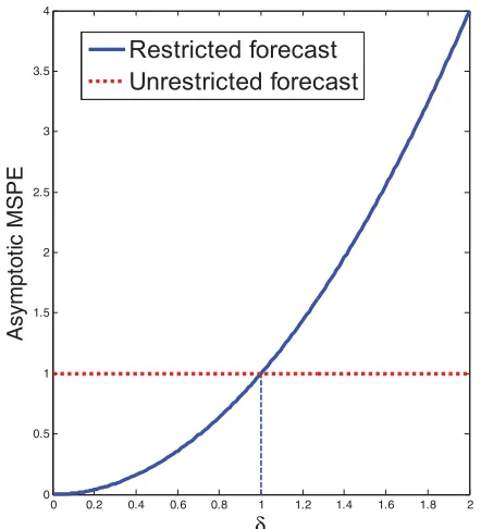
It is useful to compare the asymptotic MSPEs of these two forecasts. The MSPE can be expressed as the sum of the forecast variance and the squared forecast bias. The restricted forecast has zero variance by construction for all values ofδ, but is biased away from the optimal forecast byδ, so its MSPE isδ2. The unrestricted forecast in contrast has zero bias, but a constant variance for all δ,which can be normalized to unity without loss of generality. As Figure 1 illustrates, the MSPEs of the two forecasts are equal for δ=1. This means that for values
© 2015American Statistical Association Journal of Business & Economic Statistics January 2015, Vol. 33, No. 1 DOI:10.1080/07350015.2014.969430 Color versions of one or more of the figures in the article can be found online atwww.tandfonline.com/r/jbes.
0 0.2 0.4 0.6 0.8 1 1.2 1.4 1.6 1.8 2
Figure 1. Asymptotic MSPEs under local-to-zero asymptotics. Notes: Adapted from Inoue and Kilian (2004).δdenotes the Pitman drift term. The variance has been normalized to 1 without loss of gen-erality. The asymptotic MSPEs are equal atδ=1,not atδ=0,so a test ofH0:α=0 is not a test of the null hypothesis of equal MSPEs.
of 0< δ <1, the restricted forecast actually is more accurate than the unrestricted forecast, although the restricted forecast is based on a model that is invalid in population, given that
δ >0.This observation illustrates that there is a fundamental difference between the objective of selecting the true model and selecting the model with the lowest MSPE (also see Inoue and Kilian 2006).
Traditional tests of the null hypothesis of no predictability (referred to asold school WCMtests by Diebold) correspond to tests ofH0:β =0 which is equivalent to testingH0:δ=0. It has been common for proponents of such old school tests to advertise their tests as tests of equal forecast accuracy. This lan-guage is misleading. AsFigure 1shows, testing equal forecast accuracy under quadratic loss corresponds to testingH0:δ =1 in this example. An immediate implication ofFigure 1 is that
the critical values of conventional pseudo-out-of-sample tests of equal forecast accuracy are too low, if the objective is to compare the forecasting accuracy of the restricted and the unre-stricted forecast. As a result, these tests invariably reject the null of equal forecast accuracy too often in favor of the unrestricted forecast. They suffer from size distortions even asymptotically. This point was first made in Inoue and Kilian (2004) and has become increasingly accepted in recent years (e.g., Giacomini and White 2006; Clark and McCracken2012). It applies not only to all pseudo-out-of-sample tests of predictability published as of 2004, but also to the more recently developed alternative test of Clark and West (2007). Although the latter test embodies an explicit adjustment for finite-sample parameter estimation un-certainty, it is based on the sameH0:β=0 as more traditional tests of no predictability and hence is not suitable for evaluating the null of equal MSPEs.
BACK TO THE ROOTS
Diebold makes the case that we should return to the roots of this literature and abandon old school WCM tests in favor of the original DM test to the extent that we are interested in testing the null hypothesis of equal MSPEs. Applying the DM test relies on Assumption DM which states that the loss differential has to be covariance stationary for the DM test to have an asymptotic N(0,1) distribution. Diebold suggests that as long as we carefully test that assumption and verify that it holds at least approximately, the DM test should replace the old school WCM tests in practice. He acknowledges that in some cases there are alternative tests of the null of equal out-of-sample MSPEs such as Clark and McCracken (2011,2012), which he refers to asnew school WCMtests, but he considers these tests too complicated to be worth considering in practice.
It is useful to examine this proposal within the context of our local-to-zero predictive model. Table 1 investigates the size of the DM test based on the N(0,1) asymptotic ap-proximation. We focus on practically relevant sample sizes. In each case, we choose β in the data-generating process such that the MSPEs of the restricted and the unrestricted model are equal. Under our assumptions β =1/T1/2 under this null hypothesis. We focus on recursive estimation of the unrestricted model. The initial recursive estimation window consists of the first R sample observations, R < T . We
ex-Table 1. Size of nominal 5% DM test under local-to-zero asymptotics
T
NOTE: All results based on 50,000 trials under the null hypothesis of equal MSPEs in population. The DM test statistic is based on recursive regressions.Rdenotes the length of the initial recursive sample andTthe sample size.
plore two alternative asymptotic thought experiments. In the first case,R∈ {15,30,45}is fixed with respect to the sample size. In the second case,R=π T withπ∈ {0.25,0.5,0.75}.
Table 1 shows that, regardless of the asymptotic thought experiment, the effective size of the DM test may be lower or higher than the nominal size, depending on R and T .
In most cases, the DM test is conservative in that its em-pirical size is below the nominal size. This is an interest-ing contrast to traditional tests of H0:β=0 whose size in-variably exceeds the nominal size when testing the null of equal MSPEs. When the empirical size of the DM test ex-ceeds its nominal size, the size distortions are modest and vanish for larger T . Table 1 also illustrates that in practice
R must be large relative to Tfor the test to have reasonably accurate size. Otherwise the DM test may become extremely conservative.
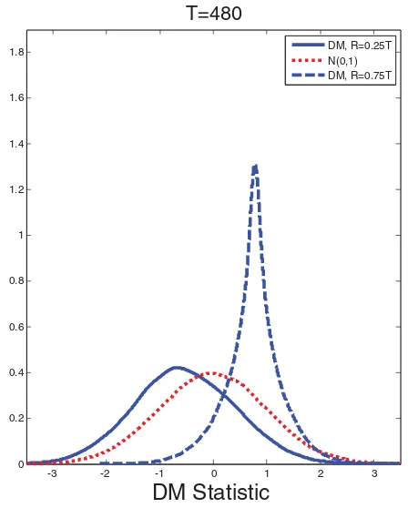
This evidence does not mean that the finite-sample distribu-tion of the DM test statistic is well approximated by a N(0,1) distribution. Figure 2 illustrates that even for T =480 the density of the DM test statistic is far from N(0,1). This finding is consistent with the theoretical analysis in Clark and McCracken (2011, p. 8) of the limiting distribution of the DM test statistic in the local-to-zero framework. Nevertheless, the right tail of the empirical distribution is reasonably close to that of the N(0,1) asymptotic approximation for largeR/T , which explains the fairly accurate size inTable 1forR=0.75T .
The failure of the N(0,1) approximation in this example suggests a violation of Assumption DM. This fact raises the
-3 -2 -1 0 1 2 3
Figure 2. Gaussian kernel density estimates of the null distribution of the DM test statistics in the local-to-zero model. Notes: Estimates based on recursive forecast error sequences based on an initial window ofRobservations. All results are based on 50,000 trials.
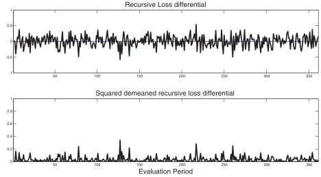
question of whether one would have been able to detect this problem by plotting and analyzing the recursive loss differential, as suggested by Diebold. The answer for our data-generating process is sometimes yes, but often not. While there are some draws of the loss differential in the Monte Carlo study that show clear signs of nonstationarity even without formal tests, many others do not. Figure 3 shows one such example. This finding casts doubt on our ability to verifyAssumption DMin practice.
Leaving aside the question of the validity of the N(0,1) ap-proximation in this context, the fact that the DM test tends to be conservative for typical sample sizes raises concerns that the DM test may have low power. It, therefore, is important to compare the DM test to the bootstrap-based tests of the same null hypothesis of equal MSPEs developed in Clark and Mc-Cracken (2011). The latternew school WCMtests are designed for nested forecasting models and are motivated by the same local-to-zero framework we relied on in our example. They can be applied to estimates of the MSPE based on rolling or recursive regressions.
Simulation results presented in Clark and McCracken (2011) suggest that their alternative tests have size similar to the DM-test in practice, facilitating the comparison. Clark and Mc-Cracken’s bootstrap-based MSE−t test in several examples appears to have slightly higher power than the DM test, but the power advantages are not uniform across all data gener-ating processes. Larger and more systematic power gains are obtained for their bootstrap MSE−F test, however. This evi-dence suggests that there remains a need for alternative tests of the null hypothesis of equal MSPEs such as the MSE−F -test in Clark and McCracken (2011). While such -tests so far are not available for all situations of interest in prac-tice, their further development seems worthwhile. There is also an alternative test of equal forecast accuracy proposed by Giacomini and White (2006), involving a somewhat different specification of the null hypothesis, which is designed specif-ically for pseudo-out-of-sample forecasts based on rolling regressions.
An interesting implication of closely related work in Clark and McCracken (2012) is that even when one is testing the null hypothesis of equal MSPEs of forecasts from nested models (as opposed to the traditional null hypothesis of no predictabil-ity), in-sample tests have higher power than the corresponding pseudo-out-of-sample tests in Clark and McCracken (2011). This finding closely mirrors the earlier results in Inoue and Kil-ian (2004) for tests of the null of no predictability. It renews the question raised in Inoue and Kilian (2004) of why anyone would care to conduct pseudo-out-of-sample inference about forecasts as opposed to in-sample inference. Professor Diebold is keenly aware of this question and draws attention to the importance of assessing and understanding the historical evolution of the accu-racy of forecasting models as opposed to their MSPE. A case in point is the analysis in Baumeister, Kilian, and Lee (2014) who show that the accuracy of forecasts with low MSPEs may not be stable over time. Such analysis does not necessarily require formal tests, however, and existing tests for assessing stability are not designed to handle the real-time data constraints in many economic time series. Nor do these tests allow for iterated as opposed to direct forecasts.
50 100 150 200 250 300 350 -1
-0.5 0 0.5 1
Recursive Loss differential
50 100 150 200 250 300 350
0 0.2 0.4 0.6 0.8 1
Squared demeaned recursive loss differential
Evaluation Period
Figure 3. Assessing assumption DM. Notes: Loss differential obtained from a random sample of lengthT−RwithT =480 andR=0.25T .
THE PROBLEM OF SELECTING FORECASTING MODELS
This leaves the related, but distinct, question of forecast-ing model selection. It is important to keep in mind that tests for equal forecast accuracy are not designed to select among alternative parametric forecasting models. This distinction is sometimes blurred in discussions of tests of equal predic-tive ability. Forecasting model selection involves the rank-ing of candidate forecastrank-ing models based on their perfor-mance. There are well-established methods for selecting the forecasting model with the lowest out-of-sample MSPE, pro-vided that the number of candidate models is small relative to the sample size, that we restrict attention to direct fore-casts, and that there is no structural change in the out-of-sample period.
It is important to stress that consistent model selection does not require the true model to be included among the forecasting models in general. For example, Inoue and Kil-ian (2006) proved that suitably specified information criteria based on the full sample will select the forecasting model with the lowest out-of-sample MSPE even when all candidate mod-els are misspecified. In contrast, forecasts obtained by ranking models by their rolling or recursive MSPE with positive prob-ability will inflate the out-of-sample MSPE under conventional asymptotic approximations. Diebold’s discussion is correct that PLS effectively equals the SIC under the assumption that R
does not depend on T , but the latter nonstandard asymptotic thought experiment does not provide good approximations in finite samples, as shown in Inoue and Kilian (2006). Moreover, consistently selecting the forecasting model with the lowest MSPE may require larger penalty terms in the information cri-terion than embodied in conventional criteria such as the SIC and AIC.
The availability of these results does not mean that the prob-lem of selecting forecasting models is resolved. First, asymp-totic results may be of limited use in small samples. Second, information criteria are not designed for selecting among a large-dimensional set of forecasting models. Their asymptotic validity breaks down, once we examine larger sets of candidate models. Third, standard information criteria are unable to handle iterated forecasts. Fourth, Inoue and Kilian (2006) proved that no fore-casting model selection method in general remains valid in the presence of unforeseen structural changes in the out-of-sample period. The problem has usually been dealt with in the existing literature by simply restricting attention to structural changes in the past, while abstracting from structural changes in the future. Finally, there are no theoretical results on how to select among forecasting methods that involve model selection at each stage of recursive or rolling regressions. The latter situation is quite common in applied work.
CONCLUSION
The continued interest in the question of how to evaluate the accuracy of forecasts shows that Diebold and Mariano’s (1995) key insights still are very timely, even 20 years later. Although the subsequent literature in some cases followed di-rections not intended by the authors, there is a growing con-sensus on how to think about this problem and which pitfalls must be avoided by applied users. The fact that in many ap-plications in-sample tests have proved superior to simulated out-of-sample tests does not mean that there are no situations in which we care about out-of-sample inference. Important exam-ples include inference about forecasts from real-time data and inference about iterated forecasts. Unfortunately, however, ex-isting tests of equal out-of-sample accuracy are not designed to
handle these and other interesting extensions. This fact suggests that much work remains to be done for econometricians going forward.
REFERENCES
Baumeister, C., and Kilian, L. (2012), “Real-Time Forecasts of the Real Price of Oil,” Journal of Business and Economic Statistics, 30, 326– 336. [13]
Baumeister, C., Kilian, L., and Lee, T. K. (2014), “Are There Gains From Pooling Real-Time Oil Price Forecasts?”Energy Economics, 46, S33–S43. [15]
Clark, T. E., and McCracken, M. W. (2012), “In-Sample Tests of Predictive Ability: A New Approach,”Journal of Econometrics, 170, 1–14. [14,15] Clark, T. E., and West, K. W. (2007), “Approximately Normal Tests for Equal
Predictive Accuracy in Nested Models,” Journal of Econometrics, 138, 291–311. [14]
Inoue, A., and Kilian, L. (2004), “Bagging Time Series Models,” CEPR Dis-cussion Paper No. 4333. [13,14,15]
Mark, N. C. (1995), “Exchange Rates and Fundamentals: Evidence on Long-Horizon Predictability,”American Economic Review, 85, 201–218. [13]
Comment
Peter Reinhard H
ANSENDepartment of Economics, European University Institute, 50134 Florence, Italy and CREATES, Aarhus University, DK-8210 Aarhus, Denmark ([email protected])
Allan T
IMMERMANNRady School of Management, UCSD, La Jolla, CA 92093 and CREATES, Aarhus University, DK-8210 Aarhus, Denmark ([email protected])
1. INTRODUCTION
The Diebold-Mariano (1995) test has played an impor-tant role in the annals of forecast evaluation. Its simplicity— essentially amounting to computing a robustt-statistic—and its generality—applying to a wide class of loss functions—made it an instant success among applied forecasters. The arrival of the test was itself perfectly timed as it anticipated, and undoubtedly spurred, a surge in studies interested in formally comparing the predictive accuracy of competing models.1
Had the Diebold-Mariano (DM) test only been applicable to comparisons of judgmental forecasts such as those provided in surveys, its empirical success would have been limited given the paucity of such data. However, the use of the DM test to sit-uations where forecasters generate pseudo out-of-sample fore-casts, that is, simulate how forecasts could have been generated in “real time,” has been the most fertile ground for the test. In fact, horse races between user-generated predictions in which different models are estimated recursively over time, are now perhaps the most popular application of forecast comparisons.
While it is difficult to formalize the steps leading to a sequence of judgmental forecasts, much more is known about model-generated forecasts. Articles such as West (1996), McCracken (2007), and Clark and McCracken (2001, 2005) took advantage of this knowledge to analyze the effect of re-cursive parameter estimation on inference about the parameters of the underlying forecasting models in the case of nonnested models (West 1996), nested models under homoscedasticity (McCracken 2007) and nested models with heteroscedastic
1Prior to the DM test, a number of authors considered tests of forecast
encom-passing, that is, the dominance of one forecast by another; see, for example, Granger and Newbold (1977) and Chong and Hendry (1986).
multi-period forecasts (Clark and McCracken2005). These pa-pers show that the nature of the learning process, that is, the use of fixed, rolling, or expanding estimation windows, matters to the critical values of the test statistic when the null of equal predictive accuracy is evaluated at the probability limits of the models being compared. Giacomini and White (2006) devel-oped methods that can be applied when the effect of estimation error has not died out, for example, due to the use of a rolling estimation window.
Other literature, including studies by White (2000), Ro-mano and Wolf (2005), and Hansen (2005) considers forecast evaluation in the presence of a multitude of models, addressing the question of whether the best single model—or, in the case of Romano and Wolf, a range of models—is capable of beat-ing a prespecified benchmark. These studies also build on the Diebold-Mariano article insofar as they base inference on the distribution of loss differentials.
Our discussion here will focus on the ability of out-of-sample forecasting tests to safeguard against data mining. Specifically, we discuss the extent to which out-of-sample tests are less sen-sitive to mining over model specifications than in-sample tests. In our view this has been and remains a key motivation for focusing on out-of-sample tests of predictive accuracy.
© 2015American Statistical Association Journal of Business & Economic Statistics January 2015, Vol. 33, No. 1 DOI:10.1080/07350015.2014.983601 Color versions of one or more of the figures in the article can be found online atwww.tandfonline.com/r/jbes.