Full Terms & Conditions of access and use can be found at
http://www.tandfonline.com/action/journalInformation?journalCode=ubes20
Download by: [Universitas Maritim Raja Ali Haji] Date: 11 January 2016, At: 22:29
Journal of Business & Economic Statistics
ISSN: 0735-0015 (Print) 1537-2707 (Online) Journal homepage: http://www.tandfonline.com/loi/ubes20
Least Squares Inference on Integrated Volatility
and the Relationship Between Efficient Prices and
Noise
Ingmar Nolte & Valeri Voev
To cite this article: Ingmar Nolte & Valeri Voev (2012) Least Squares Inference on Integrated Volatility and the Relationship Between Efficient Prices and Noise, Journal of Business & Economic Statistics, 30:1, 94-108, DOI: 10.1080/10473289.2011.637876
To link to this article: http://dx.doi.org/10.1080/10473289.2011.637876
View supplementary material
Published online: 22 Feb 2012.
Submit your article to this journal
Article views: 269
View related articles
Supplementary materials for this article are available online. Please go tohttp://tandfonline.com/r/JBES
Least Squares Inference on Integrated Volatility
and the Relationship Between Efficient Prices
and Noise
Ingmar N
OLTEWarwick Business School, Finance Group, Financial Econometrics Research Centre (FERC), Coventry, CV4 7AL ([email protected])
Valeri V
OEVSchool of Economics and Management, Aarhus University, 8000 Aarhus C, Denmark ([email protected])
The expected value of sums of squared intraday returns (realized variance) gives rise to a least squares regression which adapts itself to the assumptions of the noise process and allows for joint inference on integrated variance (IV), noise moments, and price-noise relations. In the iid noise case, we derive the asymptotic variance of the IV and noise variance estimators and show that they are consistent. The joint estimation approach is particularly attractive as it reveals important characteristics of the noise process which can be related to liquidity and market efficiency. The analysis of dependence between the price and noise processes provides an often missing link to market microstructure theory. We find substantial differences in the noise characteristics of trade and quote data arising from the effect of distinct market microstructure frictions. This article has supplementary material online.
KEY WORDS: High-frequency data; Jumps; Market microstructure; Realized volatility; Subsampling.
1. INTRODUCTION
Financial prices observed at high frequencies are known to exhibit nonmartingale features often attributed to the so-called market microstructure (MMS) noise. We provide a least squares (LS) framework for the joint estimation of the integrated vari-ance (IV) of the latent efficient price process and the parame-ters related to the characteristics of the noise process, based on realized-type statistics computed at different frequencies. The noise process is of interest in itself as highlighted in the works of Hansen and Lunde (2006), Bandi and Russell (2006b), and Oomen (2005), among others. A¨ıt-Sahalia and Yu (2009) found that the magnitude of noise is related to an array of measures of assets’ liquidity. By having a joint model, we can learn about market microstructure rather than simply treating it as noise. The observed price process is composed of signal plus noise, whose interplay is clearly important in terms of our understanding of financial markets.
The estimator we propose can be classified as a subsam-pling estimator, very much in the spirit of the two-scale re-alized volatility (TSRV) of Zhang, Mykland, and A¨ıt-Sahalia
(2005), the multiscale realized volatility (MSRV) of Zhang
(2006), and the multiscale discrete sine transform (MS-DST)
estimator of Corsi and Curci (2006). Other consistent
ap-proaches are the realized kernels (RK) of Barndorff-Nielsen
et al. (2008), which have been shown to be related to the
multiscale approach, and the preaveraging methodology of Jacod et al. (2009). It should be noted that the possibility of ordinary least squares (OLS) estimation of IV has been
ad-dressed in an independent study of Corsi and Curci (2006).
However, their main focus remained on the discrete sine trans-form of multiscale volatility measures and on iid noise spec-ifications. We relate our results to theirs throughout the
arti-cle and highlight the differences (both theoretically and in the simulations).
For the simplest case of iid noise, we derive the asymptotic variance of the IV and noise variance estimators, and provide explicit rules for the optimal choice of the number of frequen-cies. The analysis is then extended to the case of dependent, but exogenous to the efficient price, noise process for which the regression equation is augmented so that the autocovari-ance function of the noise is identified jointly with the IV. We introduce an analytical tool related to the so-called volatility signature plots (VSP), theQ-plot, which is a graphical repre-sentation of the estimates of IV against the lag length of the noise autocovariance, used to guide the variable selection in the OLS regression.
We further argue that an exogenous noise specification is not suitable if we work with midquote prices and develop a styl-ized model of incomplete price adjustment which can explain the puzzling downward bias of realized volatility (RV) found
in, for example, Hansen and Lunde (2006) and in our
empir-ical work. The price adjustment mechanism is captured by a parameter which reflects how much of the efficient price move is incorporated into the observed price. Values smaller than 1 lead to a negative RV bias as the number of observations be-comes large. We show how the proposed OLS regression can be adapted to estimate the parameter in question and report em-pirical estimates consistent with the downward-sloping VSPs obtained with midquote data.
© 2012American Statistical Association Journal of Business & Economic Statistics
January 2012, Vol. 30, No. 1 DOI:10.1080/10473289.2011.637876
94
Another feature of financial prices that we analyze is the presence of jumps. By using a jump-robust realized measure such as (staggered) bipower variation as a dependent variable in our regression, we can identify the contribution of the diffusive component, the IV, and of the jump component, the jump varia-tion (JV), to the total variavaria-tion of the process. We indicate how a noise-robust jump test can be performed but leave the theoretical treatment of the problem for further research. More importantly, our technique is the first to our knowledge that allows forjoint jump-robust estimationof the IV and the noise variance parame-ter. The potential of the LS methodology cannot be exhausted in a single study. While we focus on variance estimation and noise properties, one could possibly derive corresponding OLS re-gressions for other functionals of the diffusive component such as integrated quarticity, etc. The framework can also be extended to covariance estimation with nonsynchronous observations and
MMS noise as shown in Nolte and Voev (2008).
To evaluate the finite-sample performance of the proposed methodology and benchmark it against other existing tech-niques, we conduct an extensive simulation experiment. The results indicate that the precision of our estimators is compara-ble, and in many cases superior to that of the competing meth-ods. We conduct an empirical analysis based on 27 stocks from the DJIA index traded on New York Stock Exchange (NYSE) and National Association of Securities Dealers Automated Quo-tations (NASDAQ). In order to assess the robustness of the procedure, we compare IV estimates based on transaction and midquote data which align closely, although the noise in both types of data is of a very different nature.
The article is structured as follows: in Section 2 we intro-duce the notation, the theoretical framework, and the estimation methodology, Sections 3 and 4 contain our simulation and em-pirical results, and Section 5 concludes. Proofs are collected in an online appendix.
2. THEORETICAL SETUP
The basic assumption is that we have irregularly spaced ob-servations of a one-dimensional continuous time process pt,
t≥0, which is a noisy signal for an underlying processp∗
t:
pt =p∗t +ut,
whereutis the noise term. The processpt∗satisfies the following
assumption:
Assumption 1. The processp∗
t = t
0σudWu is a stochastic
volatility Brownian martingale process, whereσt is a c´adl´ag
stochastic process and{Wt :t ≥0}is a standard Brownian
mo-tion which is independent ofσtfor allt.
This assumption rules out leverage effects, and is needed so that we can condition on the volatility path. We expect our results to hold even in the presence of a leverage effect (indicated by our simulation results), but this would make the proofs more difficult. The integrated variation process of p∗ is given by
IVt=
for example, a trading day. Henceforth, we assume that the
period of interest is a trading day witha=0 andb=1, and we will omitaandbin the notation.
2.1 IID Noise
With respect to the noise process, we start off with the fol-lowing assumption:
Assumption 2. The noise process ut satisfies the following
conditions:
While this assumption is unrealistic from an empirical point of view, it is a convenient starting point for analyzing our method-ology and establishing an asymptotic theory.
Consider an asset with N observations (transactions, quote updates) within the period of interest. The grid of observation times{tj}j=1,...,N, which we assume to be nonrandom, is divided
into subgrids {tj s+h}j=0,...,⌊N−h
s ⌋, where s=1, . . . , S and h= 1, . . . , s. Here,{tj s+h}j=0,...,⌊N−h
s ⌋denotes thehth subgrid for a
sampling frequency of sticks (e.g., with s=2, we can have
two subgrids: the first one comprising the times{t1, t3, t5, . . .}, and the second – the times{t2, t4, t6, . . .}). In the following, we index variables at timestj simply byjto ease the notation. For
each subgrid, we define the corresponding observed, efficient, and noises-tick returns forj =1, . . . ,⌊N−sh⌋as
rj s+h≡pj s+h−p(j−1)s+h, rj s∗+h≡pj s∗+h−p∗(j−1)s+h,
ej s+h≡uj s+h−u(j−1)s+h.
Since we allow for nonequidistantly spaced observations, we need to make some assumptions regarding their regularity. Sim-ilar to Zhang (2006), we make the following assumption.
Assumption 3. The observation times {tj}j=1,...,N are
non-random and satisfy maxj|tj −tj−1| =O(1/N) as N → ∞. Furthermore, the quadratic variation of time, H(t) (see
Myk-land and Zhang (2006) and Zhang (2006) for a discussion
of this concept), defined as H(t)=limN→∞Ntj≤t(tj− tj−1)2 exists and is continuously differentiable with derivative
H′(t).
Assumption 3 effectively excludes the case of random and endogenous times, whose effect on realized variance has been studied in Li et al. (2009). Denote the number of returns on the
hths-tick subgrid asNh,s= ⌊N−sh⌋ −1. We define the realized
variance as a function of the number of returns on this subgrid as
Under Assumptions 1–3, it holds that, conditional on the volatility path (henceforth, all expectations are conditional on the volatility path),
ERVh,s(Nh,s)=IV+2Nh,sω2, (1)
a result found in Hansen and Lunde (2006) and Bandi and Russell (2006b). On the basis of the theoretical relationship in Equation (1), we can derive an OLS regression of the form
yh,s =c+β0Nh,s+εh,s, s=1, . . . , S, h=1, . . . , s,
(2) where yh,s=RVh,s(Nh,s), and the number of observations is
S(S+1)/2. In the above regression, ˆcand ˆβ0 estimate IV and 2ω2, respectively. Since the regressors are nonstochastic, endo-geneity problems are precluded. Note that irrespective of the degree of irregularity of the observation times, the variation in the regressorNh,sis mainly acrosss=1, . . . , S, and that there
is only little variation for a fixedsforh=1, . . . , sexcept for the effect of rounding. The following theorem states the variance of
ˆ
cas an estimator of IV.
Theorem 1. LetN → ∞andS=αNβ for α >0 andβ mines which term dominates the expression asymptotically.
To gain more insight into the result mentioned above, we discuss a corollary of Theorem 1.
Corollary 1.
(a) The highest speed of convergence of the estimator ˆc
is achieved whenN1−2β(ln(N))−2
Minimizing this expression with respect toαgivesα∗=
3 (b) Assuming further a normal distribution (κ=1) for the
noise process, we have that a=12ω4 and a∗ =8ω4. Substituting in the expressions for η, δ results in η=
8ω4(π2
The optimalα, minimizing the expression above, is given by
Note thatα∗is a noise-to-signal ratio, a quantity which plays
a role in the selection of subgrids and kernel length in the MSRV and RK methods.
The OLS estimator has a slightly stronger convergence com-pared to the TSRV, but does not achieve the optimal√4
N
con-vergence of the MSRV and the RK. Given that we have het-eroscedastic error terms, a weighed LS can achieve faster con-vergence. Our aim in this article, however, is not to propose the ultimate integrated variance estimator, but rather to develop a flexible framework for disentangling efficient price and noise moments. Also, asymptotic results for slowly converging esti-mators can be a poor guide to their finite-sample performance. Our simulations show that the OLS-RV estimator is in fact not worse than the above-mentioned asymptotically more efficient methods.
It is interesting to examine in more detail the relationship
between our OLS, Corsi and Curci’s (2006) multiscale least
squares (MSLS), and the MSRV estimator. All three estimators can be written in the form
that is, as weighted averages of RV statistics, where the weights
ws are constant for h=1, . . . , s. The only difference
be-tween the approaches is in the weights that have the properties
S
three estimators, but behave differently as functions ofs. For the
OLS estimator, the weights can be written asAB−ACN/s(see
the proof of Theorem 1 for the exact expressions forA,B, and
Cwhich depend onS, but are constant for eachs=1, . . . , S).
The MSRV weights are defined in Zhang (2006) as weights on
averages1ssh=1RVh,s(Nh,s) and are quadratic ins. In the form
we have written the estimator, it follows from Equations (24) and (25) in Zhang (2006) that the weights on the individual RVh,s(Nh,s) are linear ins. Finally, the MSLS weights differ
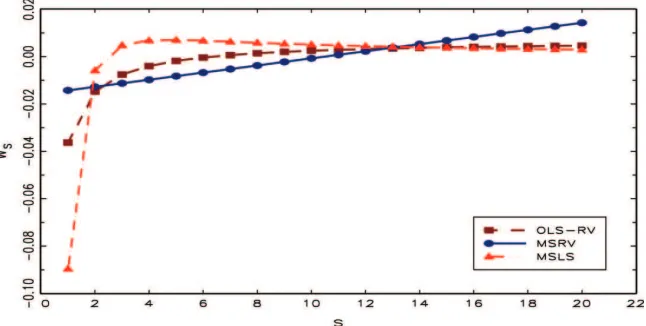
from our OLS weights since for the MSLS approach one uses again averages oversas regressors. The sequence of weights for the OLS, the MSRV, and the MSLS estimators is plotted in Fig-ure 1. The lack of asymptotic efficiency of the OLS estimator is due to the fact thatwsare not linear insand as such underweigh
RVh,s for small and larges, and overweigh RVh,s for sin the middle range. As mentioned above, a weighted LS regression can make the estimator more efficient. To follow up on this idea, note that the leading term in the variance of RVh,s behaves as
1/s. Weighting by√simplies linear weightsABs−ACN. Assuming a normal distribution for the noise, the expression forα∗in Corollary 1(b) depends only onIQandω2. Having pre-liminary estimates for these quantities thus makes our approach operational. In terms of practical implementation, we suggest usingβN = 23(1−ln(ln(ln(NN)))), rather than its limitβ=2/3, since
ln(ln(N))
ln(N) converges to zero extremely slowly. Taking this into
Figure 1. Weightswsfor the OLS-RV, the MSLS estimator of Corsi and Curci (2006), and the MSRV estimator fors=1, . . . ,20. Note that
for eachs, there aresvalues ofws(forh=1, . . . , s) which are plotted as a single point. The online version of this figure is in color.
account in the calculation of α∗, we recommend in finite
samples:
αN∗ = 3
15ω4π2−4γ2 0 +2γ1
βN2IQ .
Regression (2) delivers another interesting statistic: ˆω2=
ˆ
β0/2 as an estimator ofω2. Since the noise variance is an im-portant quantity, we derive the variance of ˆω2in the following theorem.
Theorem 2. LetN → ∞andS=αNβ forα >0 andβ ∈
[0.5,1). The variance of ˆω2is given by
var[ ˆω2]= 1 4
a∗N−1+c
∗α3 30β2N
3β−1
(ln(N))−2
+o(N−1)+oN3β−1(ln(N))−2.
The two terms in the first bracket are of the same order,O(N−1), ifβ = 23(1+ln(ln(ln(NN)))). It follows that for β <
2 3(1+
ln(ln(N)) ln(N) ), we have Var[ ˆω2]= 4aN∗ +o(N−
1
). In the case of normal noise (κ=1), a∗=8ω4, and the asymptotic variance of ˆω2 can be written as limN→∞Var[N1/2ωˆ2]=2ω4.
The noise variance estimator ˆω2converges at the parametric
speed √N and has the same asymptotic variance as the ML
estimator derived in A¨ıt-Sahalia, Mykland, and Zhang (2005), wheneverβ < 23(1+ln(ln(ln(NN)))). Theorem 2 implies that choosing
βN = 23(1−ln(ln(ln(NN))))< 23(1+ln(ln(ln(NN)))) falls also in the optimal
range forβin terms of estimatingω2.
2.2 Dependent Noise
We consider two types of dependence: in clock time, and in tick time. We believe that the concept of clock-time dependence is new and define it here.
2.2.1 Dependence in Clock Time. In high-frequency datasets, observation times are always rounded to the near-est value of some minimal time increment (e.g., a second or a millisecond). Let τ =1,2, . . . , τmax denote the clock time whereτmax is the maximal value of the clock for the observed
sample. For example, with NYSE TAQ data, observation times are typically recorded as seconds elapsed since the opening of the exchange (9:30 EST). Since the NYSE is open for 6.5 hours, a dataset containing observations of a single day has
τmax=23,400. Until now, we worked with transaction timestj
which were standardized to take values in the interval [0,1], so thattj =1/2 implies a transaction that occurred in the middle
of the trading day. We denote the clock time of the transaction by τj =tjτmax so that continuing with the previous example
τj =11,700. For an arbitraryt∈[0,1], we defineτ = ⌈t τmax⌉, where ⌈x⌉denotes the nearest integer larger or equal to x. At actual transaction timestj, we do not need the rounding, since
all transactions are recorded as a multiple of a minimal time in-crement. The clock-time-dependent noise satisfies the following assumption:
Assumption 4. The noise process ut is dependent in clock
time if
(a) ps∗⊥⊥ut, for allsandt;
(b) E[ut]=0, for all t;
(c) ut is covariance stationary with autocovariance function
given byγ(q)=E[uτuτ−q],τ = ⌈t τmax⌉,q=1,2, . . ..
Clock-time dependence is not the same as calendar-time de-pendence, since the lag q is not a fixed interval of calendar time. Thus,q=5 can represent 5-second or 5-millisecond de-pendence. Clock-time dependence has some of the features of
calendar-time dependence (since q is a measure of physical
time) and of tick-time dependence discussed below (since it scales with the resolution of the time stamps and thus implicitly with trading activity). The dependence structure is only defined at the times at which the noise actually occurs (integer-valued
q), thus having an advantage over calendar-time dependence
which should be defined for any real q. The advantage over
tick-time dependence is that markets do operate in physical time; a 1-second tick and a 1-minute tick are rather different in terms of the amount of information processed by the market over the particular time interval, and so it is to be expected that the dependence structure in the noise process should take this into account. We now consider the implications of clock-time
dependence for our regression framework. Under Assumptions sult is a straightforward extension of Equation (1) taking into account that under Assumption 4, var[ej s+h]=2(γ(0)−γ(q)),
where q=τj s+h−τ(j−1)s+h. The approximation in Equation
(4) results from truncating the autocorrelation function at lag
Q. The equation could be made exact if one explicitly assumes
γ(q)=0 forq > Q, for some positiveQ. In terms of practi-cal implementation,Qhas to be chosen by the econometrician, an issue we revisit later. The OLS regression corresponding to Equation (4) takes the form
yh,s =c+β′xh,s +εh,s, s=1, . . . , S, h=1, . . . , s, note that clock-time dependence is applicable directly for a mul-tivariate process. This is not the case for tick-time dependence, which is discussed in the following section.
2.2.2 Dependence in Tick Time. The tick-time-dependent noise satisfies the following assumption.
Assumption 5. The noise processutis dependent in tick time
if
(a) ps∗⊥⊥ut, for allsandt;
(b) E[ut]=0, for allt;
(c) ut is covariance stationary with autocovariance function
given byγ(q)=E[ujuj−q].
The difference with respect to clock-time dependence is that
qnow measures the number of ticks rather than the number of
time units between two observations. Under Assumptions 1, 3, and 5, we have that
and thus γ(0)−γ(s) cannot be identified without additional assumptions. A possible identifying assumption is to postulate thatγ(q)=0 forq≥Q¯ for some ¯Q >0. Then fors≥Q¯, we
which is essentially the iid noise framework (since in this case
γ(0)=ω2), where we have assumed that the noise in ¯Q-tick re-turns can be considered to be iid. Given the evidence in Hansen and Lunde (2006), ¯Qcan be chosen so that there is approx-imately 1 minute between returns. The iid noise theory can then be applied to the resulting ¯Q-tick returns. As an alterna-tive, if ¯Qis too large compared to an optimally selectedS, we recommend using some sparse sampling (as the approximately 1-minute sampling in Barndorff-Nielsen et al. (2008)) and ap-plying the OLS regression for the iid noise case to the sparse returns.
2.3 Endogenous Noise
We motivate the idea of endogenous noise from a market mi-crostructure perspective. A feature of high-frequency data is that prices do not always fully reflect all available information. This phenomenon is observed, for example, in the trading model of Campbell, Lo, and MacKinlay (1997) based on regular sampling in the absence of trading activity. As Bandi and Russell (2006a) argued, midquotes can be sticky at high frequencies implying observed zero returns. One possibility for writing a model of this kind is to assume thatpj =pj−1+φrj∗. In this model, the
full information returnr∗
j is only partially incorporated in the
current observed pricepj. Whenφ=0, prices are sticky and
observed returns are zero. A problem with this specification is that it implies uj =(φ−1)p∗j. Since both the efficient price
and noise are ˆIto processes, the variation ofp∗
j anduj is not
identifiable, a problem which is stressed by A¨ıt-Sahalia, Myk-land, and Zhang (2006). In order to have an identifiable model which allows for partial incorporation of information, we define observed prices as
pj =pj∗−1+φrj∗+νj, (7)
whereφ plays the same role as above andνj is an additional
source of noise, which we assume to be iid with mean zero and varianceω2. Clearly, the caseν
j =0 can be considered as a
spe-cial case. The equation above implies thatuj =(φ−1)rj∗+νj,
a version of the specification suggested by Hansen and Lunde (2006). In this respect, what we propose here is an intuitive refor-mulation of their specification, where the parameterφrepresents the degree of information processing. Ifφ=1, then all infor-mation is incorporated fully anduj is an iid process. The
im-plication of this noise specification for our OLS methodology is the following: On the tick frequency (full grid), the return noise process is given byej =(φ−1)(rj∗−rj∗−1)+νj −νj−1. It
fol-sds. The full-grid realized variance is given by
RV(N)=Nj=1(rj∗ 2
+2r∗
jej +ej2), and thus
E [RV(N)]=IV+2φ(φ−1)IV+2N ω2, (8)
where we have used as an approximationNj=1σ 2
j−1=IV. If prices adjust incompletely to the new information,φ∈[0,1) so thatφ(φ−1)≤0, whileφ >1 would imply price overreaction. Note that the polynomialφ(φ−1) is symmetric aroundφ=0.5 so that for identification purposes, we restrict the range ofφto
φ≥0.5. To provide an intuition of why this arises, assume
for a moment that νj =0, and consider the casesφ=1 and
φ=0, both of which lead toφ(φ−1)=0. These two cases are (almost) indistinguishable in terms of their impact on the bias of RV, since in the first case we observe the efficient price process without noise, while in the second case, we have a one-tick delay, that is, we observep∗
j−1attj. Thus, in the latter case, we
observe again allr∗
j, with the exception of the last returnrN∗. The
approximationNj=1σj2−1=IV makes both cases identical.
In order to analyze the impact of specification (7) on
our OLS regression, we need to derive E[RVh,s(Nh,s)]. We
have that by definition ej s+h=uj s+h−u(j−1)s+h, which in
this case results in ej s+h=(φ−1)(rj s∗+h,1−r(∗j−1)s+h,1)+
νj s+h−ν(j−1)s+h, where rj s∗+h,1=p∗j s+h−pj s∗+h−1 is a
one-tick return contrary to the s-tick return which we have
de-fined earlier asrj s∗+h≡pj s∗+h−p∗(j−1)s+h(and analogously for
sds. It is important to stress that the dependence
oper-ates at the highest frequency, as a result of which the identifiabil-ity problems mentioned above do not arise. Using the definition of the sparse-grid RV, it follows that
ERVh,s(Nh,s)
we reconcile this with the downward sloping VSP obtained
for midquote data in Hansen and Lunde (2006) (and also in
our empirical analysis below)? We argue that specification (7) can be seen as an encompassing model for which the restric-tionω2
=0 represents a model suitable for midquotes and the restrictionφ=1 is representative for trade data. Specifying dif-ferent models for both types of data can be further motivated by the empirical studies of Dacorogna et al. (2001), Barndorff-Nielsen et al. (2009), and Oomen (2010), among others, doc-umenting differences in the properties of transaction versus midquote returns. Theoretically, one can substitute the assump-tionω2
=0 for midquote data with local-to-zero asymptotics of the typeω2
=ω02N−αwithα
≥1 and a constantω02, discussed by Barndorff-Nielsen et al. (2008). As they noted, however, this is essentially equivalent to theω2=0, that is, no noise, case. In this sense, assumingω2=0 is a simple way of formalizing that the predominant source of noise in midquotes is due to
incom-plete price adjustment, consistent with downward-sloping VSP. As far as transaction data are concerned, the assumptionφ=1 is inconsequential because as soon as there is an exogenous (not necessarily iid) noise component of orderO(1), it dominates the effect of endogeneity of the type we have assumed. This follows up to a first-order approximation
for some constantζ. Using this approximation, we can write
ERVh,s(Nh,s)≈IV+Nh,s(2ω2+ζ /N).
It is clear that the slope coefficient in the OLS regression (2) now estimates (2ω2
+ζ /N) which converges to 2ω2 as
N → ∞, while the intercept remains a consistent estimator of IV. This analysis relates nicely to the discussion in Section 5.5 of Barndorff-Nielsen et al. (2008), who showed that the impact of a linear endogeneity model of the type (7) is asymptotically negligible in terms of estimation of IV. The above contempla-tions imply the following regression models for trade and quote data, respectively:
ERVh,s(Nh,s)=IV+2ω2Nh,s with trade data, (11)
ERVh,s(Nh,s)=IV+ζ Nh,s/N with midquote data.
(12)
Can we learn something about the price adjustment coefficient
φ from the estimate of ζ? We argue that NN
j s+h is an average per tick volatility which is then
scaled to a daily volatility byN (with constant volatility and equidistant sampling we would have equality). Given that the
Nh,s ticks are spread over the whole day (i.e., the tick at time
tj s+hcan be thought of as representative in terms of volatility for
thesticks betweent(j−1)s+handtj s+h) and that typically there is
not a large variation in durations, we think that this is a reason-able approximation. The implication is thatζ ≈2φ(φ−1)IV.
Solving forφ, we have thatφ1/2=
I V±√I V2+2I V ζ
2I V . Ifζ is
neg-ative, as we would expect for midquote data, the rootφ2<0.5, which we assumed away for identification purposes. Thus, we define an estimator ofφin terms of the coefficients in regression
model (12) as ˆφ= I V+
√
I V2+2I Vζˆ
2I V . We report estimates ofφfor
midquote data in the empirical section.
2.4 Jumps
Until now we have assumed thatp∗ has continuous sample
paths. We relax this assumption by introducing jumps into the model so that now
p∗t =
t
0
σudWu+Jt. (13)
We follow Barndorff-Nielsen and Shephard (2006) and assume
thatJtis given byJt = Nt
j=1cj, whereNtis a simple counting
process andcj are nonzero iid random variables. The quadratic
variation of p∗ can now be decomposed as a sum of the
integrated variance IV≡ut=0σ2
udu and the sum of squared
jumps JV≡Nt
j=1c 2
j. In this section, we show how one can
adapt the OLS regression (2) to estimate the integrated variance in the presence of jumps. The regression is based on the (stag-gered) bipower variation defined on the full grid as (see, e.g.,
Huang and Tauchen2005)
dard normal random variable. The case i=0 corresponds to
the “standard” bipower variation and i=1,2, . . . represents the case when the returns are staggered by iticks. The sparse subgrid version of the bipower variation is given by
BVh,si (Nh,s)=µ−12
If there is no noise and the price process is given by Equation (13), BVi(N) is a consistent estimator of IV. The effect of MMS
noise is thatrjandrj−1are correlated so that the results in Huang and Tauchen (2005) suggest that the bias of BV0(N) depends, in a complicated way, on a term measuring the expectation of the product of the absolute value of two correlated Gaussian variables. The consequence is that both ˆcand ˆω2=βˆ0/2 from regression (2) withyh,s≡BVh,s0 (Nh,s) are biased, as evidenced
in our simulation study. Given the iid noise assumption, how-ever,rj andrj−2are independent. With the additional assump-tion thatutis normally distributed, it is straightforward to show
(again, using the results in Huang and Tauchen2005) that the bias of the staggered (i=1) bipower variation is simply 2N ω2. This has the nice implication that withyh,s ≡BV
h,s
1 (Nh,s), we
obtain unbiased estimators of IV and ω2, resulting in a joint jump-robust estimation of both integrated variance and noise variance. While jump- and noise-robust approaches for the esti-mation of IV do exist (see, e.g., Podolskij and Vetter2009), we believe ours to be the first result on jump-robust joint estimation of IV andω2. As a final remark, we note that an estimator ofJV can be defined as ˆcRV−cˆBV
1, that is the difference between ˆc
in regression (2), with RV and BV1as dependent variables. The corresponding test for jumps is beyond the scope of the article and is left for further research.
3. SIMULATION EVIDENCE
We classify our estimators depending on the variable used as yh,s in Equation (2) as OLS-RV, OLS-BV0 and OLS-BV1, BV0and BV1representing bipower and staggered bipower vari-ation, respectively. To compare the finite-sample performance
of our class of estimators against other consistent estimation
techniques, namely, the MS-DST of Corsi and Curci (2006),
the MSRV of Zhang (2006), the TSRV of Zhang, Mykland,
and A¨ıt-Sahalia (2005), and the RK of Barndorff-Nielsen et al. (2008) using the modified Tukey-Hanning2kernel, we resort to Monte Carlo simulations. We employ an iid noise setup, since in this case we have an asymptotic theory for the OLS-RV, MSRV, TSRV, and the RK estimators, and a theoretically founded way of choosing an optimal number of subgrids or kernel length.
The notationSis used to denote both the number of subgrids
and the number of realized autocovariances (kernel length) in the RK framework. The simulation setup is borrowed from the
SV1FJ specification in Huang and Tauchen (2005) for which
the efficient price process is given by
dpt∗=µdt+exp(β0+β1vt)dW p∗
t +dJt, p∗0 =0,
dvt =αvvtdt+dWtv, v0=1/(−2α),
where Wp∗ and Wv are Brownian motion processes. We
al-low them to be correlated to examine whether the results are affected by the presence of a leverage effect, which was as-sumed away to facilitate the proofs of the theoretical results. Note that we also allow for drift, although in Assumption
1 we have µ=0. The parameterization is also as in Huang
and Tauchen (2005) (with some slight modifications following Barndorff-Nielsen et al. (2008)). We setµ=0.03,β1=0.125,
αv = −0.025, andβ0=β12/2αv, which is a normalization
en-suring that E[01σ2
udu]=1. The coefficient of correlation
be-tweendWtp∗anddWtvtakes values{0,−0.62}, representing the
no-leverage and leverage cases, respectively. The jump process,
Jt, is a compound Poisson process with constant jump
inten-sityλ∈ {0,0.058}(representing the no-jump and jump cases, respectively) and the jump sizescj areN(0,1). The noise
pro-cess,u(t), is iidN(0, ω2), where the size of ω2 is not defined in absolute terms, but rather in terms of the noise-to-signal
ratio ξ2=ω2/01σ4
udu for which we assign values 0.0001
(low-noise regime), 0.001 (medium-noise regime), and 0.01 (high-noise regime). We also consider the case of noise due to rounding, which is simply achieved by rounding the prices to the nearest cent. This results in 16 scenarios that are summarized inTable 1.
We conduct two experiments with 5,000 simulation runs, summarized as follows:
1. SetN =23,400 (corresponding to 6.5 hours of
second-by-second data), vary S (the number of subgrids, or kernel
length) from 2 to 100 with a step of 2 (S=2,4,6, . . . ,
100);
2. LetNvary from 1000 to 100,000 with a step of 1000, for a total of 100 values. For each of the five estimators, choose
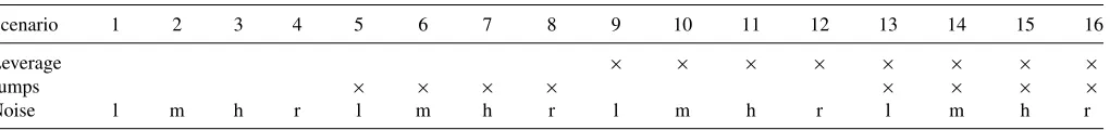
Table 1. Summary of simulation scenarios.×indicates whether the particular effect is present. l, m, h, and r represent the low, medium, high, and rounding noise scenarios, respectively
Scenario 1 2 3 4 5 6 7 8 9 10 11 12 13 14 15 16
Leverage × × × × × × × ×
Jumps × × × × × × × ×
Noise l m h r l m h r l m h r l m h r
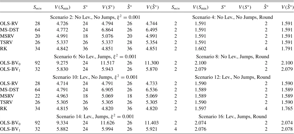
Table 2. Relative RMSEs (in percentage) of the true value of IV.Smindenotes the number of subsamples (kernel length) for which the corresponding minimum is achieved across the values ofSconsidered in the simulation,S∗denotes the asymptotically optimal number of
subsamples (kernel length) using true values of IV,IQ, andω2, and ˆS∗denotes the asymptotically optimal number of subsamples (kernel length) based on estimated values of IV,IQ, andω2, following Barndorff-Nielsen et al. (2009)
Smin V(Smin) S∗ V(S∗) Sˆ∗ V( ˆS∗) Smin V(Smin) S∗ V(S∗) Sˆ∗ V( ˆS∗)
Scenario 2: No Lev., No Jumps,ξ2
=0.001 Scenario 4: No Lev., No Jumps, Round
OLS-RV 28 4.726 24 4.794 26 4.744 2 1.591 2 1.591
MS-DST 64 4.772 24 6.864 26 6.495 2 1.591 2 1.591
MSRV 20 4.991 18 5.076 20 4.991 2 1.591 2 1.591
TSRV 26 5.337 26 5.337 28 5.354 2 1.591 2 1.591
RK 34 4.842 36 4.851 36 4.851 2 1.602 4 1.791
Scenario 6: No Lev., Jumps,ξ2
=0.001 Scenario 8: No Lev., Jumps, Round
OLS-BV0 92 9.275 24 11.517 26 11.300 2 2.100 2 2.100
OLS-BV1 32 5.830 24 5.943 26 5.870 2 2.079 2 2.079
Scenario 10: Lev., No Jumps,ξ2
=0.001 Scenario 12: Lev., No Jumps, Round
OLS-RV 28 4.714 24 4.791 26 4.733 2 1.590 2 1.590
MS-DST 64 4.791 24 6.905 26 6.536 2 1.589 2 1.589
MSRV 22 4.963 18 5.069 18 5.069 2 1.589 2 1.589
TSRV 26 5.305 26 5.305 26 5.305 2 1.590 2 1.590
RK 34 4.815 36 4.820 36 4.820 2 1.597 4 1.765
Scenario 14: Lev., Jumps,ξ2
=0.001 Scenario 16: Lev., Jumps, Round
OLS-BV0 92 9.334 24 11.626 26 11.403 2 2.074 2 2.074
OLS-BV1 32 5.882 24 5.994 26 5.921 4 2.076 2 2.078
NOTE: Finally,V(x) is the value of the statistic (RMSE) atx. Due to the fact that in the simulations,Stakes on only even values from 2 to 100,Sminis even by construction, whileS∗
and ˆS∗are rounded to the nearest even number.
S in an optimal way, given the corresponding asymptotic
theory.
A summary of the results for the first simulation experiment is presented inTable 2for all scenarios with medium noise and rounding. Scaling the noise parameterξ2does not lead to qual-itative differences and therefore, due to space limitations, the results for the remaining scenarios are not reported here but are available from the authors upon request. In each scenario, we first report the value ofSthat minimized the root mean squared error (RMSE) in the simulations (Smin) and the associated value
of the RMSE. To address the applicability of the asymptotically optimal rule for choosingS, we further report the infeasible
S∗, assuming that ω2
and IQ (and where necessary IV) are
known, the feasible ˆS∗ with estimated plug-in quantities, and
the associated RMSEs. Corsi and Curci (2006) did not provide a rule for their estimator but, as it is a regression-type estimator,
we use the optimalS for our OLS estimator given in
Corol-lary 1, which is also used for the OLS-BV0 and the OLS-BV1
estimators. If the source of noise is rounding, the true value of
ω2is not available and hence the corresponding columns in the table are missing. The results for the jump-robust estimators are only reported in the scenarios with jumps. In these scenarios, the other estimators measure the total quadratic variation and are thus biased forIV. It is immediately clear from the table that leverage does not play an important role.
Rounding can be seen as representative of a very small nonnormal iid noise effect and, as such, is handled quite well. As expected from the theoretical analysis in Section 2.4 the OLS-BV0is biased for IV, which is the reason for the fairly large
RMSE. The OLS-BV1estimates IV very well, even though
com-pared to the OLS-RV in the absence of jumps, there is a small
loss of efficiency. Interestingly, the asymptotically optimal rule for the choice ofS∗works rather well, although there is some
scope for improvement in the lines of Bandi and Russell (2008, 2009), who suggest a finite-sample RMSE correction forS∗.
Finally, it is evident that “borrowing” the value ofS∗and using
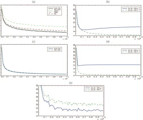
it for the MS-DST as well as for the OLS-BV estimators is not a good idea so that developing some sort of optimal rule of choice would greatly improve their performance. Given the robustness with respect to leverage and thatξ2 =0.001 is considered rep-resentative, for the second simulation experiment, we choose scenarios 2 and 6. The results are illustrated in Figure 2. In panel (a), we compare the OLS-RV against the four competing estimators. The RMSEs of the RK and the OLS-RV are almost identical (the lines practically overlap) with both estimators out-performing the TSRV, the MSRV, and the MS-DST. As we saw in Experiment 1, the performance of the MS-DST depends on the right choice ofS, for which we do not have a selection crite-rion. Panel (b) compares our jump-robust estimators for which it is again evident that the OLS-BV0is biased while the
OLS-BV1 achieves a very low RMSE. Panels (c) and (d) illustrate
the RMSE of the estimators forω2 in the absence/presence of jumps.
As Theorem 2 shows, the OLS-RV estimator forω2is√N
-consistent and, thus, much more precise than the estimator forIV
for largeN, which is also the case for the MS-DST estimator. In the presence of jumps, as discussed in Section 2.4 the OLS-BV0 is biased for ω2 and, therefore, the RMSE does not converge.
As claimed, the OLS-BV1 delivers a jump-robust estimate of
ω2 which appears to be consistent. In panel (e), we look at
the RMSE of the differences ˆcRV−cˆBV
0 and ˆcRV−cˆBV1 as
estimators forJV. The estimator based on BV1performs well as expected.
Figure 2. Summary of the results for simulation Experiment 2. Each panel illustrates the percentage RMSE of various estimators as a function ofNfor (a) IV in the absence of jumps, (b) IV in the presence of jumps, (c)ω2in the absence of jumps, (d)ω2in the presence of jumps, and (e) JV. The online version of this figure is in color.
4. EMPIRICAL ANALYSIS
In this section, we apply the LS estimation framework to high-frequency data (trades and quotes) of 27 stocks for the period April 1, 2004, to July 31, 2008. We refer the reader to Barndorff-Nielsen et al. (2009) for a description of the data cleaning procedures. The ticker symbols used in the study can be found in the first column ofTable 3. The first 25 stocks trade on NYSE and the last 2 on NASDAQ.
An empirical application of the LS estimation methodology as proposed in this article requires a choice ofQandS. While
we provide an indication of how to chooseS in Corollary 1,
the choice of Q should be data driven as it depends on the
strength of the serial dependence of the noise process. In or-der to analyze this dependence, we propose a graphical tool, theQ-plot, very similar to the VSP mentioned in Section 2. A
Q-plot is a plot of the estimate of IV orω2 againstQfrom the regression in Equation (5), arising from the relation in Equation
(4). To ensure sufficient counts Nh,s(q), q=1, . . . , Q when
Qis large (we letQ go up to 30), we use an arbitrary larger value ofS=50, and we note that while a suboptimally chosen
S might increase the variance of the estimator, it cannot lead to serious biases. TheQ-plots are a guide for the value of Q
which should be chosen in practice so that the resulting esti-mate of IV is (at least approxiesti-mately) unbiased. IfQis chosen too large relative to the strength of the dependence inu, then the estimate will be unbiased but its standard error will be in-creased (inclusion of irrelevant regressors). If, on the contrary,
Q is chosen too small relative to the strength of the
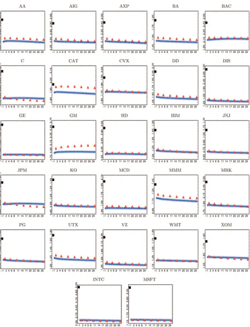
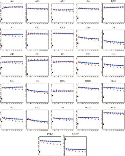
depen-dence inu, then the estimate will be biased (omitted variable bias). As an alternative, a suitable value forQcan be deduced from autocorrelations of returns. Figures3 and4 are collec-tions ofQ-plots for the 27 stocks in our study for the trade and quote data, respectively. For comparison, we also compute the realized Parzen kernel as recommended in Barndorff-Nielsen et al. (2009), with data sampled at ticks at approximately Q
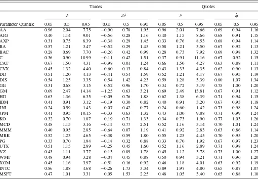
Table 3. Results from the OLS regression (2) applied to the model in Equations (11) and (12)
Trades Quotes
ˆ
c ωˆ2 cˆ φˆ
Parameter Quantile 0.05 0.5 0.95 0.05 0.5 0.95 0.05 0.5 0.95 0.05 0.5 0.95 AA 0.96 2.04 7.75 −0.90 0.78 1.95 0.96 2.01 7.66 0.69 0.94 1.16 AIG 0.40 1.14 9.01 −0.56 0.28 1.16 0.40 1.15 8.66 0.68 0.91 1.15 AXP 0.31 0.75 8.39 −0.38 0.29 1.45 0.33 0.76 8.53 0.68 0.94 1.14 BA 0.57 1.21 3.47 −0.52 0.29 1.45 0.58 1.21 3.50 0.67 0.92 1.13 BAC 0.28 0.69 7.70 −0.26 0.42 0.99 0.28 0.73 7.92 0.69 0.98 1.32 C 0.36 0.90 10.99 −0.11 0.42 1.51 0.37 0.91 11.16 0.67 0.92 1.15 CAT 0.67 1.50 4.31 −0.98 0.01 1.24 0.66 1.50 4.27 0.63 0.88 1.11 CVX 0.45 1.32 4.40 −0.60 0.13 0.84 0.43 1.33 4.35 0.62 0.90 1.13 DD 0.51 1.20 4.13 −0.41 0.54 1.59 0.52 1.21 4.17 0.67 0.95 1.19 DIS 0.54 1.25 3.35 0.54 1.42 4.23 0.59 1.28 3.39 0.80 1.07 1.34 GE 0.31 0.68 3.15 0.52 0.96 1.70 0.34 0.72 3.19 0.75 1.00 1.20 GM 0.69 2.47 14.14 −1.25 0.63 3.21 0.69 2.49 13.81 0.67 0.91 1.12 HD 0.63 1.36 6.35 −0.09 0.76 1.88 0.62 1.38 6.39 0.71 0.94 1.15 IBM 0.41 0.91 3.12 −0.19 0.30 0.82 0.40 0.91 3.20 0.67 0.93 1.18 JNJ 0.24 0.59 1.43 0.07 0.42 0.77 0.24 0.60 1.42 0.73 0.98 1.24 JPM 0.41 0.95 10.15 −0.33 0.63 1.32 0.43 1.00 9.88 0.71 0.99 1.24 KO 0.32 0.70 1.87 0.19 0.71 1.33 0.34 0.73 1.90 0.77 1.03 1.26 MCD 0.48 1.15 3.16 −0.14 0.77 2.51 0.52 1.16 3.14 0.70 1.01 1.24 MMM 0.40 0.95 2.85 −0.64 0.07 1.19 0.41 0.92 2.83 0.63 0.86 1.14 MRK 0.52 1.23 4.65 −0.38 0.59 1.80 0.55 1.25 4.45 0.70 0.95 1.20 PG 0.33 0.70 1.94 −0.14 0.32 0.88 0.33 0.70 1.92 0.67 0.97 1.23 UTX 0.51 1.15 2.89 −0.25 0.45 1.60 0.52 1.16 2.89 0.71 0.98 1.24 VZ 0.43 1.11 3.77 0.13 0.89 1.78 0.45 1.12 3.78 0.73 1.00 1.27 WMT 0.48 0.94 3.28 −0.04 0.45 0.88 0.50 0.94 3.21 0.71 0.96 1.20 XOM 0.45 1.16 3.97 −0.51 0.16 0.92 0.46 1.18 4.01 0.63 0.92 1.19 INTC 0.86 1.88 4.68 −0.26 1.73 3.34 0.89 1.97 4.80 0.65 0.87 1.07 MSFT 0.47 1.01 3.31 0.05 1.53 2.25 0.48 1.05 3.40 0.65 0.88 1.10
NOTE: The estimates ofω2are scaled by 104. For each parameter, we report the 5% median and 95% quantile of the distribution across days for the full sample of 1,152 days.
seconds apart for Q=1,5,10,15,20,25,30 (Barndorff-Nielsen et al. (2009) recommended using all data, which cor-responds in our plots to the kernel atQ=1). As a benchmark, we also report the standard RV using all data which is plot-ted for convenience atQ= −1. A clear difference between the plots based on transaction data and the plots based on quote data is that both the OLS-RV estimator and the RK are con-siderably more stable when applied to transaction data. Fur-thermore, the full-grid RV is always upward biased with trade data, while it is almost always downward biased with midquote
data. It can be clearly observed fromFigure 3 that Q=0 is
a very reasonable choice with trade data, which is also con-firmed by the close match with the RK using all data. We do not report standard errors but, given the confidence intervals reported in Barndorff-Nielsen et al. (2008), the differences be-tween the OLS and the kernel estimates are not significant. Choosing a larger value ofQhardly changes the estimate, while it most likely increases the variance as discussed above. Thus, while noise in trade data might not be iid, it seems that its iid component is overwhelmingly dominating in terms of biasing the RV at very high frequencies. Fine tuning the estimator to take potential non-iid features of the noise into account ap-pears redundant. The explanation for the downward bias of RV with midquote data, put forward in Section 2.3 was that with midquotes the dominating source of noise is the incomplete
price adjustment mechanism. We examine this phenomenon in more detail shortly.
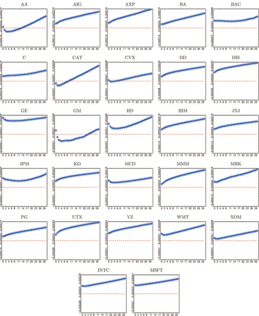
Concerning the noise variance, if the noise is iid, theQ-plot should remain flat as ˆω2 is unbiased for allQ. If, on the con-trary, the noise follows an MA( ˜Q) process, then the estimate of ˆω2will be biased in all regressions for whichQ <Q˜ due to omission of relevant variables. This analysis is meaningful for trade data for which an exogenous noise component seems to be a good description. For midquote data, we have advocated an endogenous noise specification, and therefore, we only analyze theQ-plots for trade data, collected inFigure 5. The plots reveal that the iid assumption is an oversimplification as the estimate ofω2is increasing inQ. In particular, for smaller values ofQ, ˆω2
is downward biased. Based on the theory of omitted variables, we know that the bias is determined by the sign of the correla-tion of the omitted variable with the included variable and the sign of the coefficient on the omitted variable. Given that the regressor related toβ0,Nh,s, is positively related to the
regres-sors Nh,s(q) (the more the observations, the more will be the
counts for eachq), and the omitted variables have coefficients
−2γ(q), we conclude thatγ(q) is generally positive. This phe-nomenon is consistent with price impacts of large trades which can cause a temporary deviation of the observed price from its efficient level in one direction (a cluster of positive or neg-ative noise terms), an effect which iid noise cannot capture.
Figure 3. Q-plots for IV with transaction data against values ofQranging from 0 to 30 (pluses). The RV estimator using all available data is plotted for comparison at−1 (square). Realized kernels with data sampled at approximatelyQseconds using the Parzen kernel are plotted for values ofQ=1,5,10,15,20,25,30 (triangles). All plots are averages over the whole sample (1,152 days). The online version of this figure is in color.
Figure 4. Q-plots for IV with midquote data against values ofQranging from 0 to 30 (pluses). The RV estimator using all available data is plotted for comparison at−1 (square). Realized kernels with data sampled at approximatelyQseconds using the Parzen kernel are plotted for values ofQ=1,5,10,15,20,25,30 (triangles). All plots are averages over the whole sample (1,152 days). The online version of this figure is in color.
Figure 5. Q-plots forω2with midquote data against values ofQranging from 0 to 30. The dashed line is at zero for each plot. All plots are averages over the whole sample (1,152 days). The online version of this figure is in color.
Comparing theQ-plots for the integrated variance against the
Q-plots forω2 (Figures3and5), there seems to be a contra-diction: the estimates of IV are largely unaffected by increasing
Qbeyond 0, while ˆω2 is rather sensitive. We provide two ex-planations to resolve this issue: First, we argue that magnitude plays a role. The varianceω2is of the same order of magnitude as the autocovariancesγ(q), while the integrated variance is of a much larger magnitude. Second, which is a more compelling theoretical argument, omitted variable bias can be decomposed as the product of the coefficients of the regression of the omit-ted variables on the included variables and the coefficients on the omitted variables. Let us consider what happens whenQis increased fromQ=0 toQ=1. The biases of ˆcand ˆβ0then de-pend on the coefficients of the regression ofNh,s(1) (the omitted
variable) on a constant andNh,s (the included variables). The
intercept of this regression will, in population, be zero, as for
Nh,s =0, anyNh,s(q),q >0 will necessarily be zero as well,
while the slope coefficient will be positive since, as mentioned above,Nh,s is positively related to the regressorsNh,s(q). Thus,
there is a strong theoretical reason why the estimate ofω2is bi-ased, while the estimate of integrated variance is not. This type of argument naturally carries over for anyQ >0. Admitting that Q=0 is likely not the best choice in terms of estimat-ingω2, we focus our analysis on further issues and setQ=0 henceforth.
To study the incomplete price adjustment mechanism
pro-posed in Section 2.3 and to assess the robustness of the IV
estimator to different noise characteristics, we estimate Equa-tions (11) and (12). SettingQ=0 allows us to use our optimal rule forS∗ in Corollary 1, which is what we do in our further
analysis. InTable 3, we present summarized results for the pa-rameter estimates of the regression (2) applied to the model in Equations (11) and (12) for trade and quote data, respectively. For each coefficient, we report the 5% quantile, median and across the days in the sample. First, we note that the distri-bution of ˆcacross days with trade data is very similar to the one obtained with quote data, which implies that the estimator is robust to various noise effects. The median of the coeffi-cient of price adjustment,φ, is smaller than 1 for 22 out of the 27 stocks, which is in line with the theoretical argumentation implying that on more than half of the days the prices incorpo-rated new information with a delay. Interestingly, the two NAS-DAQ stocks do not appear to have significantly different values ofφ.
This lends support to the hypothesis that the “sluggishness” in midquotes is likely due to the asynchronous movement of the bid and ask prices causing staggered adjustment and thus a pure artefact of the way midquote prices are calculated. Carrying out the analysis directly on the bid and ask prices and on a much larger selection of stocks might shed more light on the possible differences between the markets. We remind that coefficients larger than 1 are still consistent with the model and indicate a partial short-term overreaction of the observed price. We note,
however, that the model proposed in Equation (7) is highly
stylized. Clearly, having a constant φ throughout the day is
not likely and a model with time-varying coefficient is arguably more realistic and an extension worth looking into. Furthermore, the calculation ofφis based on an approximation, which might be better on certain days and worse on others.
5. CONCLUSION
The article proposes an LS regression for the estimation of integrated volatility and noise moments of stochastic volatility martingales observed with noise, based on sampling the process at different frequencies. In the case of iid noise, we derive the asymptotic properties of the estimators and provide a rule for choosing the optimal (in a RMSE sense) number of frequencies. The framework is then extended to cover the case of dependent and endogenous noise and jumps. Further extensions of the pro-posed methodology are possible, once it is recognized that it relies on a moment condition which can be derived for other functionals of the volatility, for example, integrated quarticity, or integrated covariation in the case of higher-dimensional pro-cesses, the latter being undertaken in Nolte and Voev (2008).
The finite-sample properties of the estimators are examined in a Monte Carlo simulation, confirming its precision relative to other approaches in the extant literature. Empirically, we find that suitable specifications of the model can accommodate the characteristics of transaction and midquote prices, and can ex-plain the differences in the noise process present in both types of data. We argue that an iid noise component is dominant in transaction prices, while for midquotes a more involved endoge-nous noise specification based on partial price adjustment seems more suitable.
SUPPLEMENTARY MATERIALS
Supplementary materials containing the proofs to Theorems 1 and 2, as well Corollary 1, are available online.
ACKNOWLEDGMENTS
We would like to thank Peter Hansen, Wolfgang H¨ardle, Ilze Kalnina, Asger Lunde, Mark Podolskij, Kevin Sheppard, and Almut Veraart for helpful discussions. All remaining errors are ours. The work has been supported in part by the Euro-pean Community’s Human Potential Program under contract HPRN-CT-2002-00232, Microstructure of Financial Markets in Europe; and by the Fritz Thyssen Foundation through the project “Dealer-Behavior and Price-Dynamics on the Foreign Exchange Market”. Financial support by the Center for Research in Econometric Analysis of Time Series, CREATES, funded by the Danish National Research Foundation, is gratefully acknowledged.
[Received May 2009. Accepted April 2011.]
REFERENCES
A¨ıt-Sahalia, Y., Mykland, P. A., and Zhang, L. (2005), “How Often to Sample a Continuous-Time Process in the Presence of Market Microstructure Noise,” Review of Financial Studies, 18(2), 351–416. [97]
A¨ıt-Sahalia, Y., Mykland, P., and Zhang, L. (2006), “Comment on Realized Vari-ance and Market Microstructure Noise,”Journal of Business and Economic Statistics, 24(2), 162–167. [98]
A¨ıt-Sahalia, Y., and Yu, J. (2009), “High Frequency Market Microstructure Noise Estimates and Liquidity Measures,”Annals of Applied Statistics, 3(1), 422–457. [94]
Bandi, F. M., and Russell, J. R. (2006a), “Comment on Realized Variance and Market Microstructure Noise,”Journal of Business and Economic Statistics, 24(2), 167–173. [98]
—— (2006b), “Separating Microstructure Noise from Volatility,”Journal of Financial Economics, 79(3), 655–692. [94,96]
—— (2008), “Microstructure Noise, Realized Variance, and Optimal Sam-pling,”Review of Economic Studies, 75(2), 339–369. [101]
—— (2009), “Market Microstructure Noise, Integrated Variance Estimators, and the Accuracy of Asymptotic Approximation,” Working Paper, Univer-sity of Chicago, Booth School of Business. [101]
Barndorff-Nielsen, O. E., Hansen, P., Lunde, A., and Shephard, N. (2008), “Designing Realized Kernels to Measure the Ex-post Variation of Eq-uity Prices in the Presence of Noise,” Econometrica, 76, 1481–1536. [94,98,99,100,103]
—— (2009), “Realized Kernels in Practice: Trades and Quotes,”Econometrics Journal, 12(3), C1–C32. [99,102]
Barndorff-Nielsen, O. E., and Shephard, N. (2006), “Econometrics of Testing for Jumps in Financial Economics Using Bipower Variation,”Journal of Financial Econometrics, 4(1), 1–30. [99]
Campbell, J. Y., Lo, A. W., and MacKinlay, A. C. (1997), The Econo-metrics of Financial Markets, Princeton NJ: Princeton University Press. [98]
Corsi, F., and Curci, G., (2006), “Discrete Sine Transform for Multi-Scales Realized Volatility Measures,” Working Paper, University of Lugano. [94,96,100,101]
Dacorogna, M. M., Genc¸ay, R., M¨uller, U. A., Olsen, R. B., and Pictet, O. V. (2001)An Introduction to High-Frequency Finance, San Diego, CA: Academic Press. [99]
Hansen, P. R., and Lunde, A. (2006), “Realized Variance and Market Mi-crostructure Noise,” Journal of Business and Economic Statistics, 24, 127–161. [94,96,98,99]
Huang, X., and Tauchen, G. (2005), “The Relative Contribution of Jumps to Total Price Variance,”Journal of Financial Econometrics, 3(4), 456–499. [100,100]
Jacod, J., Li, Y., Mykland, P. A., Podolskij, M., and Vetter, M. (2009), “Mi-crostructure Noise in the Continuous Case: The Pre-averaging Approach,” Stochastic Processes and Their Applications, 119(7), 2249–2276 [94] Li, Y., Mykland, P. A., Renault, E., Zhang, L., and Zheng, X. (2009),
“Real-ized Volatility When Sampling Times can be Endogenous.” Working Paper, University of Chicago. [95]
Mykland, P. A., and Zhang, L. (2006), “ANOVA for Diffusions and Ito Pro-cesses,”The Annals of Statistics, 34(4), 1931–1963. [95]
Nolte, I., and Voev, V. (2008), “Estimating High-Frequency Based (Co-) Vari-ances: A Unified Approach,” CREATES Working Paper 2008-31, Aarhus University. [95,107]
Oomen, R. C. A. (2005), “Properties of Bias-Corrected Realized Variance Under Alternative Sampling Schemes,”Journal of Financial Econometrics, 3, 555–577. [94]
—— (2010), “Zero Intelligence Realized Variance Estimation,”Finance and Stochastics, 14(2), 249–283. [99]
Podolskij, M., and Vetter, M. (2009), “Estimation of Volatility Functionals in the Simultaneous Presence of Microstructure Noise and Jumps,”Bernoulli, 15(3), 634–658. [100]
Zhang, L. (2006), “Efficient Estimation of Stochastic Volatility Using Noisy Observations: A Multi-Scale Approach,”Bernoulli, 12, 1019–1043. [94,95,96,100]
Zhang, L., Mykland, P. A., and A¨ıt-Sahalia, Y. (2005), “A Tale of Two Time Scales: Determining Integrated Volatility With Noisy High Frequency Data,” Journal of the American Statistical Association, 100, 1394–1411. [94,100]