a short introduction to probability

(1)

A Short Introduction to

Probability

Prof. Dirk P. Kroese Department of Mathematics

c

(2)

(3)

Preface

These notes form a comprehensive 1-unit (= half a semester) second-year in-troduction to probability modelling. The notes are not meant to replace the lectures, but function more as a source of reference. I have tried to include proofs of all results, whenever feasible. Further examples and exercises will be given at the tutorials and lectures. To completely master this course it is important that you

1. visit the lectures, where I will provide many extra examples;

2. do the tutorial exercises and the exercises in the appendix, which are there to help you with the “technical” side of things; you will learn here to apply the concepts learned at the lectures,

3. carry out random experiments on the computer, in the simulation project. This will give you a better intuition about how randomness works.

All of these will be essential if you wish to understand probability beyond “filling in the formulas”.

Notation and Conventions

Throughout these notes I try to use a uniform notation in which, as a rule, the number of symbols is kept to a minimum. For example, I prefer qij to q(i, j),

Xt to X(t), andEX to E[X].

The symbol “:=” denotes “is defined as”. We will also use the abbreviations r.v. for random variable and i.i.d. (or iid) for independent and identically and distributed.

(6)

Numbering

All references to Examples, Theorems, etc. are of the same form. For example, Theorem 1.2 refers to the second theorem of Chapter 1. References to formula’s appear between brackets. For example, (3.4) refers to formula 4 of Chapter 3.

Literature

• Leon-Garcia, A. (1994). Probability and Random Processes for Electrical Engineering, 2nd Edition. Addison-Wesley, New York.

• Hsu, H. (1997). Probability, Random Variables & Random Processes. Shaum’s Outline Series, McGraw-Hill, New York.

• Ross, S. M. (2005). A First Course in Probability, 7th ed., Prentice-Hall, Englewood Cliﬀs, NJ.

• Rubinstein, R. Y. and Kroese, D. P. (2007). Simulation and the Monte Carlo Method, second edition, Wiley & Sons, New York.

(7)

Chapter 1

Random Experiments and

Probability Models

1.1 Random Experiments

The basic notion in probability is that of a random experiment: an experi-ment whose outcome cannot be determined in advance, but is nevertheless still subject to analysis.

Examples of random experiments are:

1. tossing a die,

2. measuring the amount of rainfall in Brisbane in January,

3. counting the number of calls arriving at a telephone exchange during a fixed time period,

4. selecting a random sample of fifty people and observing the number of left-handers,

5. choosing at random ten people and measuring their height.

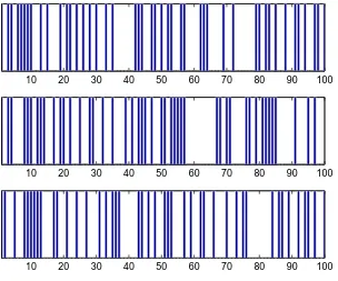
Example 1.1 (Coin Tossing) The most fundamental stochastic experiment is the experiment where a coin is tossed a number of times, sayntimes. Indeed, much of probability theory can be based on this simple experiment, as we shall see in subsequent chapters. To better understand how this experiment behaves, we can carry it out on a digital computer, for example in Matlab. The following simple Matlab program, simulates a sequence of 100 tosses with a fair coin(that is, heads and tails are equally likely), and plots the results in a bar chart.

(8)

Here x is a vector with 1s and 0s, indicating Heads and Tails, say. Typical outcomes for three such experiments are given in Figure 1.1.

10 20 30 40 50 60 70 80 90 100

Figure 1.1: Three experiments where a fair coin is tossed 100 times. The dark bars indicate when “Heads” (=1) appears.

We can also plot the average number of “Heads” against the number of tosses. In the same Matlab program, this is done in two extra lines of code:

y = cumsum(x)./[1:100] plot(y)

(9)

1.1 Random Experiments 7

Example 1.2 (Control Chart) Control charts, see Figure 1.3, are frequently used in manufacturing as a method for quality control. Each hour the average output of the process is measured — for example, the average weight of 10 bags of sugar — to assess if the process is still “in control”, for example, if the machine still puts on average the correct amount of sugar in the bags. When the process> Upper Control Limitor <Lower Control Limit and an alarm is raised that the process is out of control, e.g., the machine needs to be adjusted, because it either puts too much or not enough sugar in the bags. The question is how to set the control limits, since the random process naturally fluctuates around its “centre” or “target” line.

(10)

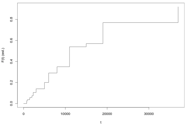
Example 1.3 (Machine Lifetime) Suppose 1000 identical components are monitored for failure, up to 50,000 hours. The outcome of such a random experiment is typically summarised via the cumulative lifetime table and plot, as given in Table 1.1 and Figure 1.3, respectively. Here ˆF(t) denotes the proportion of components that have failed at time t. One question is how ˆF(t) can be modelled via a continuous function F, representing the lifetime distribution of a typical component.

t(h) failed F(t) 0 0 0.000 750 22 0.020 800 30 0.030 900 36 0.036 1400 42 0.042 1500 58 0.058 2000 74 0.074 2300 105 0.105

t (h) failed F(t) 3000 140 0.140 5000 200 0.200 6000 290 0.290 8000 350 0.350 11000 540 0.540 15000 570 0.570 19000 770 0.770 37000 920 0.920

Table 1.1: The cumulative lifetime table

t

F(t) (est.)

0 10000 20000 30000

0.0

0.2

0.4

0.6

0.8

(11)

1.1 Random Experiments 9

Example 1.4 A 4-engine aeroplane is able to fly on just one engine on each wing. All engines are unreliable.

Figure 1.5: A aeroplane with 4 unreliable engines

Number the engines: 1,2 (left wing) and 3,4 (right wing). Observe which engine works properly during a specified period of time. There are 24 = 16 possible outcomes of the experiment. Which outcomes lead to “system failure”? More-over, if the probability of failure within some time period is known for each of the engines, what is the probability of failure for the entire system? Again this can be viewed as a random experiment.

Below are two more pictures of randomness. The first is a computer-generated “plant”, which looks remarkably like a real plant. The second is real data depicting the number of bytes that are transmitted over some communications link. An interesting feature is that the data can be shown to exhibit “fractal” behaviour, that is, if the data is aggregated into smaller or larger time intervals, a similar picture will appear.

Figure 1.6: Plant growth

125 130 135 140 145 150 155

0 2000 4000 6000 8000 10000 12000 14000

Interval

number of bytes

Figure 1.7: Telecommunications data

(12)

1.2 Sample Space

Although we cannot predict the outcome of a random experiment with certainty we usually can specify a set of possible outcomes. This gives the first ingredient in our model for a random experiment.

Definition 1.1 The sample spaceΩ of a random experiment is the set of all possible outcomes of the experiment.

Examples of random experiments with their sample spaces are:

1. Cast two dice consecutively,

Ω =_{(1,1),(1,2), . . . ,(1,6),(2,1), . . . ,(6,6)_}.

2. The lifetime of a machine (in days),

Ω =R+=_{positive real numbers _}.

3. The number of arriving calls at an exchange during a specified time in-terval,

Ω =_{0,1,_{· · · }}=Z+.

4. The heights of 10 selected people.

Ω =_{(x1, . . . , x10), xi ≥0, i= 1, . . . ,10}=R10+ .

Here (x1, . . . , x10) represents the outcome that the length of the first se-lected person isx1, the length of the second person isx2, et cetera.

Notice that for modelling purposes it is often easier to take the sample space larger than necessary. For example the actual lifetime of a machine would certainly not span the entire positive real axis. And the heights of the 10 selected people would not exceed 3 metres.

1.3 Events

Often we are not interested in a single outcome but in whether or not one of a group of outcomes occurs. Such subsets of the sample space are calledevents. Events will be denoted by capital letters A, B, C, . . . . We say that event A

(13)

1.3 Events 11

Examples of events are:

1. The event that the sum of two dice is 10 or more,

A={(4,6),(5,5),(5,6),(6,4),(6,5),(6,6)}.

2. The event that a machine lives less than 1000 days,

A= [0,1000).

3. The event that out of fifty selected people, five are left-handed,

A=_{5_}.

Example 1.5 (Coin Tossing) Suppose that a coin is tossed 3 times, and that we “record” every head and tail (not only the number of heads or tails). The sample space can then be written as

Ω ={HHH, HHT, HT H, HT T, T HH, T HT, T T H, T T T},

where, for example, HTH means that the first toss is heads, the second tails, and the third heads. An alternative sample space is the set {0,1}3 _{of binary} vectors of length 3, e.g., HTH corresponds to (1,0,1), and THH to (0,1,1). The eventA that the third toss is heads is

A={HHH, HT H, T HH, T T H}.

Since events are sets, we can apply the usual set operations to them:

1. the setA∪B (A unionB) is the event thatA or B or both occur, 2. the setA_∩B (AintersectionB) is the event that AandB both occur, 3. the eventAc (A complement) is the event thatA does not occur, 4. if A_⊂B (Ais a subsetofB) then event A is said toimplyevent B. Two events Aand B which have no outcomes in common, that is, A_∩B =_∅, are calleddisjointevents.

Example 1.6 Suppose we cast two dice consecutively. The sample space is Ω = _{(1,1),(1,2), . . . ,(1,6),(2,1), . . . ,(6,6)_}. Let A = _{(6,1), . . . ,(6,6)_} be the event that the first die is 6, and let B = _{(1,6), . . . ,(1,6)_} be the event that the second dice is 6. ThenA∩B ={(6,1), . . . ,(6,6)}∩{(1,6), . . . ,(6,6)}=

(14)

It is often useful to depict events in aVenn diagram, such as in Figure 1.8

Figure 1.8: A Venn diagram

In this Venn diagram we see

(i) A_∩C =_∅ and therefore events A and C are disjoint.

(ii) (A_∩Bc₎_∩₍_Ac_∩_B_{) =}_∅_{and hence events} _A_∩_Bc _and_Ac_∩_B _{are disjoint.}

Example 1.7 (System Reliability) In Figure 1.9 three systems are depicted, each consisting of 3 unreliable components. Theseriessystem works if and only if (abbreviated as iff)allcomponents work; theparallelsystem works iffat least oneof the components works; and the 2-out-of-3 system works iff at least 2 out of 3 components work.

1 2 3

Series

1

2

3

Parallel

2

3

2 3

1 1

2-out-of-3 Figure 1.9: Three unreliable systems

Let Ai be the event that the ith component is functioning,i= 1,2,3; and let

Da, Db, Dc be the events that respectively the series, parallel and 2-out-of-3

system is functioning. Then,

Da=A1∩A2∩A3 , and

(15)

1.4 Probability 13

Also,

Dc = (A1∩A2∩A3)∪(Ac1∩A2∩A3)∪(A1∩Ac2∩A3)∪(A1∩A2∩Ac3) = (A1∩A2)∪(A1∩A3)∪(A2∩A3).

Two useful results in the theory of sets are the following, due toDe Morgan: If_{Ai}is a collection of events (sets) then

This is easily proved via Venn diagrams. Note that if we interpret Ai as the

event that a component works, then the left-hand side of (1.1) is the event that the corresponding parallel system is not working. The right hand is the event that at all components are not working. Clearly these two events are the same.

1.4 Probability

The third ingredient in the model for a random experiment is the specification of the probability of the events. It tells us howlikelyit is that a particular event will occur.

Definition 1.2 A probability P is a rule (function) which assigns a positive number to each event, and which satisfies the followingaxioms:

Axiom 1: P(A)≥0.

Axiom 2 just states that the probability of the “certain” event Ω is 1. Property (1.3) is thecrucialproperty of a probability, and is sometimes referred to as the sum rule. It just states that if an event can happen in a number of diﬀerent waysthat cannot happen at the same time, then the probability of this event is simply the sum of the probabilities of the composing events.

(16)

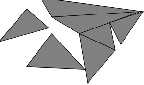
Figure 1.10: The probability measure has the same properties as the “area” measure: the total area of the triangles is the sum of the areas of the idividual triangles.

is how you should interpret property (1.3). But instead of measuring areas, P measures probabilities.

As a direct consequence of the axioms we have the following properties for P.

Theorem 1.1 Let Aand B be events. Then,

1. P(∅) = 0.

2. A_⊂B =_⇒P(A)_≤P(B). 3. P(A)_≤1.

4. P(Ac) = 1₋P(A).

5. P(A∪B) =P(A) +P(B)−P(A∩B).

Proof_.

1. Ω = Ω ∩ ∅ ∩ ∅ ∩ · · ·, therefore, by the sum rule,P(Ω) =P(Ω) +P(∅) + P(_∅) +_{· · ·}, and therefore, by the second axiom, 1 = 1 +P(_∅) +P(_∅) +_{· · ·}, from which it follows thatP(_∅) = 0.

2. IfA_⊂B, thenB =A_∪(B_∩Ac), whereAandB_∩Acare disjoint. Hence, by the sum rule, P(B) =P(A) +P(B_∩Ac_{), which is (by the first axiom)}

greater than or equal to P(A).

3. This follows directly from property 2 and axiom 2, since A⊂Ω.

4. Ω = A_∪Ac_{, where} _A _and _Ac _{are disjoint. Hence, by the sum rule and}

axiom 2: 1 =P(Ω) =P(A) +P(Ac), and thusP(Ac) = 1−P(A).

5. Write A_∪B as the disjoint union of A and B_∩Ac_{. Then,} _P₍_A_∪_B_{) =}

(17)

1.4 Probability 15

We have now completed our model for a random experiment. It is up to the modeller to specify the sample space Ω and probability measureP which most closely describes the actual experiment. This is not always as straightforward as it looks, and sometimes it is useful to model only certainobservations in the experiment. This is whererandom variablescome into play, and we will discuss these in the next chapter.

Example 1.8 Consider the experiment where we throw a fair die. How should we define Ω andP?

Obviously, Ω = _{1,2, . . . ,6_}; and some common sense shows that we should definePby

P(A) = |A|

6 , A⊂Ω,

where_|A_|denotes the number of elements in setA. For example, the probability of getting an even number isP({2,4,6}) = 3/6 = 1/2.

In many applications the sample space iscountable, i.e. Ω =_{a1, a2, . . . , an} or

Ω =_{a1, a2, . . .}. Such a sample space is calleddiscrete.

The easiest way to specify a probability _P on a discrete sample space is to specify first the probability pi of each elementary event {ai} and then to

define

P(A) =

i:ai∈A

pi , for all A⊂Ω.

This idea is graphically represented in Figure 1.11. Each element ai in the

sample is assigned a probability weight pi represented by a black dot. To find

the probability of the setA we have to sum up the weights of all the elements inA.

(18)

Again, it is up to the modeller to properly specify these probabilities. Fortu-nately, in many applications all elementary events are equally likely, and thus the probability of each elementary event is equal to 1 divided by the total num-ber of elements in Ω. E.g., in Example 1.8 each elementary event has probability 1/6.

Because the “equally likely” principle is so important, we formulate it as a theorem.

Theorem 1.2 (Equilikely Principle) If Ω has a finite number of outcomes, and all are equally likely, then the probability of each event Ais defined as

P(A) = |A|

|Ω_| .

Thus for such sample spaces the calculation of probabilities reduces tocounting the number of outcomes (in A and Ω).

When the sample space is not countable, for example Ω = R+, it is said to be continuous.

Example 1.9 We draw at random a point in the interval [0,1]. Each point is equally likely to be drawn. How do we specify the model for this experiment? The sample space is obviously Ω = [0,1], which is a continuous sample space. We cannot define P via the elementary events _{x_}, x _∈ [0,1] because each of these events must have probability 0 (!). However we can define P as follows: For each 0≤a≤b≤1, let

P([a, b]) =b−a .

This completely specifies P. In particular, we can find the probability that the point falls into any (suﬃciently nice) set A as thelength of that set.

1.5 Counting

Counting is not always easy. Let us first look at some examples:

1. A multiple choice form has 20 questions; each question has 3 choices. In how many possible ways can the exam be completed?

2. Consider a horse race with 8 horses. How many ways are there to gamble on the placings (1st, 2nd, 3rd).

(19)

1.5 Counting 17

4. How many diﬀerent throws are possible with 3 dice?

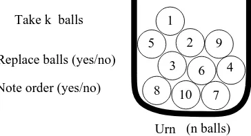
To be able to comfortably solve a multitude of counting problems requires a lot of experience andpractice, and even then, some counting problems remain exceedingly hard. Fortunately, many counting problems can be cast into the simple framework of drawing balls from an urn, see Figure 1.12.

4

2 9

1 5

3

8 ₁₀ ₇

6

Urn (n balls) Note order (yes/no)

Replace balls (yes/no) Take k balls

Figure 1.12: An urn with nballs

Consider an urn withndiﬀerent balls, numbered 1, . . . , nfrom whichkballs are drawn. This can be done in a number of diﬀerent ways. First, the balls can be drawn one-by-one, or one could draw all thekballs at the same time. In the first case the order in which the balls are drawn can be noted, in the second case that is not possible. In the latter case we can (and will) still assume the balls are drawn one-by-one, but that the order is not noted. Second, once a ball is drawn, it can either be put back into the urn (after the number is recorded), or left out. This is called, respectively, drawing with and withoutreplacement. All in all there are 4 possible experiments: (ordered, with replacement), (ordered, without replacement), (unordered, without replacement) and (ordered, with replacement). The art is to recognise a seemingly unrelated counting problem as one of these four urn problems. For the 4 examples above we have the following

1. Example 1 above can be viewed as drawing 20 balls from an urn containing 3 balls, noting the order, and with replacement.

2. Example 2 is equivalent to drawing 3 balls from an urn containing 8 balls, noting the order, and without replacement.

3. In Example 3 we take 3 balls from an urn containing 20 balls, not noting the order, and without replacement

4. Finally, Example 4 is a case of drawing 3 balls from an urn containing 6 balls, not noting the order, and with replacement.

(20)

by sets, e.g., _{1,2,3_} = _{3,2,1_}. We now consider for each of the four cases how to count the number of arrangements. For simplicity we consider for each case how the counting works for n= 4 and k = 3, and then state the general situation.

Drawing with Replacement, Ordered

Here, after we draw each ball, note the number on the ball, and put the ball back. Let n= 4, k = 3. Some possible outcomes are (1,1,1),(4,1,2), (2,3,2),

(4,2,1), . . . To count how many such arrangements there are, we can reason as follows: we have three positions (·,·,·) to fill in. Each position can have the numbers 1,2,3 or 4, so the total number of possibilities is 4_×4_×4 = 43 = 64. This is illustrated via the following tree diagram:

4 1 2 3

(3,2,1) (1,1,1)

First position

Second position Third position

1

2

3

4

For general nand k we can reason analogously to find:

The number of ordered arrangements of k numbers chosen from

{1, . . . , n_}, with replacement (repetition) is nk_.

Drawing Without Replacement, Ordered

(21)

1.5 Counting 19

size k from set _{1, . . . , n_}. (A permutation of _{1, . . . , n_} of size n is simply called a permutation of{1, . . . , n}(leaving out “of sizen”). For the 1st position we have 4 possibilities. Once the first position has been chosen, we have only 3 possibilities left for the second position. And after the first two positions have been chosen there are 2 positions left. So the number of arrangements is 4_×3_×2 = 24 as illustrated in Figure 1.5, which is the same tree as in Figure 1.5, but with all “duplicate” branches removed.

4 2 3

(3,2,1)

First position

Second position Third position

1

2

3

4

1

3 4

1 2

4

1 2

3

1 4

(2,3,1) (2,3,4)

For generaln andk we have:

The number of permutations of size k from _{1, . . . , n_} is nPk =

n(n₋1)_{· · ·}(n₋k+ 1).

In particular, when k= n, we have that the number of ordered arrangements of n items is n! = n(n₋1)(n₋2)_{· · ·}1, where n! is called n-factorial. Note that

n_P k=

n! (n₋k)!.

Drawing Without Replacement, Unordered

This time we draw k numbers from {1, . . . , n} but do not replace them (no replication), and do not note the order (so we could draw them in one grab). Taking again n = 4 and k = 3, a possible outcome is {1,2,4}, {1,2,3}, etc. If we noted the order, there would benPk outcomes, amongst which would be

(22)

arrangements without replications are called combinations of sizekfrom the set {1, . . . , n}.

To determine the number of combinations of size k simply need to divide nPk

be the number of permutations of k items, which is k!. Thus, in our example (n = 4, k = 3) there are 24/6 = 4 possible combinations of size 3. In general we have:

The number of combinations of sizek from the set_{1, . . . n_} is

n_C k=

n

k =

n_P k

k! =

n! (n₋k)!k! .

Note the two diﬀerent notations for this number. We will use the second one.

Drawing With Replacement, Unordered

Taking n = 4, k = 3, possible outcomes are {3,3,4}, {1,2,4},{2,2,2}, etc. The trick to solve this counting problem is to represent the outcomes in a diﬀerent way, via an ordered vector (x1, . . . , xn) representing how many times

an element in{1, . . . ,4}occurs. For example, {3,3,4}corresponds to (0,0,2,1) and _{1,2,4_} corresponds to (1,1,0,1). Thus, we can count how many distinct vectors (x1, . . . , xn) there are such that the sum of the components is 3, and

each xi can take value 0,1,2 or 3. Another way of looking at this is to consider

placing k= 3 balls into n= 4 urns, numbered 1,. . . ,4. Then (0,0,2,1) means that the third urn has 2 balls and the fourth urn has 1 ball. One way to distribute the balls over the urns is to distribute n−1 = 3 “separators” and

k= 3 balls overn₋1 +k= 6 positions, as indicated in Figure 1.13.

6 3 4 5 2

1

Figure 1.13: distributingkballs over nurns

The number of ways this can be done is the equal to the number of ways k

positions for the balls can be chosen out ofn−1 +kpositions, that is,n+_kk−1. We thus have:

The number of diﬀerent sets _{x1, . . . , xk} with xi ∈ {1, . . . , n},i=

1, . . . , k is

n+k₋1

(23)

1.5 Counting 21

Returning to our original four problems, we can now solve them easily:

1. The total number of ways the exam can be completed is 320= 3,486,784,401. 2. The number of placings is8_P

3 = 336.

3. The number of possible combinations of CDs is20₃= 1140. 4. The number of diﬀerent throws with three dice is 8₃= 56.

More examples

Here are some more examples. Not all problems can be directly related to the 4 problems above. Some require additional reasoning. However, the counting principles remain the same.

1. In how many ways can the numbers 1,. . . ,5 be arranged, such as 13524, 25134, etc?

Answer: 5! = 120.

2. How many diﬀerent arrangements are there of the numbers 1,2,. . . ,7, such that the first 3 numbers are 1,2,3 (in any order) and the last 4 numbers are 4,5,6,7 (in any order)?

Answer: 3!×4!.

3. How many diﬀerent arrangements are there of the word “arrange”, such as “aarrnge”, “arrngea”, etc?

Answer: Convert this into a ball drawing problem with 7 balls, numbered 1,. . . ,7. Balls 1 and 2 correspond to ’a’, balls 3 and 4 to ’r’, ball 5 to ’n’, ball 6 to ’g’ and ball 7 to ’e’. The total number of permutations of the numbers is 7!. However, since, for example, (1,2,3,4,5,6,7) is identical to (2,1,3,4,5,6,7) (when substituting the letters back), we must divide 7! by 2!×2! to account for the 4 ways the two ’a’s and ’r’s can be arranged. So the answer is 7!/4 = 1260.

4. An urn has 1000 balls, labelled 000, 001, . . . , 999. How many balls are there that have all number in ascending order (for example 047 and 489, but not 033 or 321)?

Answer: There are 10×9×8 = 720 balls with diﬀerent numbers. Each triple of numbers can be arranged in 3! = 6 ways, and only one of these is in ascending order. So the total number of balls in ascending order is 720/6 = 120.

5. In a group of 20 people each person has a diﬀerent birthday. How many diﬀerent arrangements of these birthdays are there (assuming each year has 365 days)?

(24)

Once we’ve learned how to count, we can apply the equilikely principle to calculate probabilities:

1. What is the probability that out of a group of 40 people all have diﬀerent birthdays?

Answer: Choosing the birthdays is like choosing 40 balls with replace-ment from an urn containing the balls 1,. . . ,365. Thus, our sample space Ω consists of vectors of length 40, whose components are cho-sen from {1, . . . ,365}. There are |Ω| = 36540 such vectors possible, and all are equally likely. Let A be the event that all 40 people have diﬀerent birthdays. Then, _|A_| = 365_P

40 = 365!/325! It follows that P(A) =|A|/|Ω| ≈0.109, so not very big!

2. What is the probability that in 10 tosses with a fair coin we get exactly 5 Heads and 5 Tails?

Answer: Here Ω consists of vectors of length 10 consisting of 1s (Heads) and 0s (Tails), so there are 210 of them, and all areequally likely. Let A

be the event of exactly 5 heads. We must count how many binary vectors there are with exactly 5 1s. This is equivalent to determining in how many ways the positions of the 5 1s can be chosen out of 10 positions, that is, 10₅. Consequently, P(A) =10₅/210 = 252/1024 _≈0.25.

3. We draw at random 13 cards from a full deck of cards. What is the probability that we draw 4 Hearts and 3 Diamonds?

Answer: Give the cards a number from 1 to 52. Suppose 1–13 is Hearts, 14–26 is Diamonds, etc. Ω consists of unordered sets of size 13, without repetition, e.g.,{1,2, . . . ,13}. There are|Ω|=52₁₃of these sets, and they are all equally likely. Let A be the event of 4 Hearts and 3 Diamonds. To form A we have to choose 4 Hearts out of 13, and 3 Diamonds out of 13, followed by 6 cards out of 26 Spade and Clubs. Thus, _|A_| =

₁₃

4

×13₃×26₆. So thatP(A) =|A|/|Ω| ≈0.074.

1.6 Conditional probability and independence

B A

Ω

How do probabilities change when we know some event B _⊂Ω has occurred? SupposeB

has occurred. Thus, we know that the out-come lies in B. ThenAwill occur if and only ifA_∩B occurs, and the relative chance of A

occurring is therefore

P(A∩B)/P(B).

(25)

1.6 Conditional probability and independence 23

P(A|B) = P(A∩B)

P(B) (1.4)

Example 1.10 We throw two dice. Given that the sum of the eyes is 10, what is the probability that one 6 is cast?

LetB be the event that the sum is 10,

B={(4,6),(5,5),(6,4)}.

LetA be the event that one 6 is cast,

A={(1,6), . . . ,(5,6),(6,1), . . . ,(6,5)}.

Then, A_∩B = _{(4,6),(6,4)_}. And, since all elementary events are equally likely, we have

P(A_|B) = 2/36 3/36 =

2 3.

Example 1.11 (Monte Hall Problem) This is a nice application of condi-tional probability. Consider a quiz in which the final contestant is to choose a prize which is hidden behind one three curtains (A, B or C). Suppose without loss of generality that the contestant chooses curtain A. Now the quiz master (Monte Hall) always opens one of the other curtains: if the prize is behind B, Monte opens C, if the prize is behind C, Monte opens B, and if the prize is behind A, Monte opens B or C with equal probability, e.g., by tossing a coin (of course the contestant does not see Monte tossing the coin!).

A

B

_C

Suppose, again without loss of generality that Monte opens curtain B. The contestant is now oﬀered the opportunity to switch to curtain C. Should the contestant stay with his/her original choice (A) or switch to the other unopened curtain (C)?

(26)

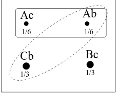
is behind C, and Monte opens B. Let A, B, C be the events that the prize is behind A, B and C, respectively. Note that A = {Ac, Ab}, B = {Bc} and

C =_{Cb_}, see Figure 1.14.

Ab

Cb Bc

1/6 1/6

1/3 1/3 Ac

Figure 1.14: The sample space for the Monte Hall problem.

Now, obviously P(A) = P(B) = P(C), and since Ac and Ab are equally likely, we have P({Ab}) = P({Ac}) = 1/6. Monte opening curtain B means that we have information that event _{Ab, Cb_} has occurred. The probability that the prize is under A given this event, is therefore

P(A|B is opened) = P({Ac, Ab} ∩ {Ab, Cb}) P({Ab, Cb}) =

P({Ab}) P({Ab, Cb}) =

1/6 1/6 + 1/3 =

1 3. This is what we expected: the fact that Monte opens a curtain does not give us any extra information that the prize is behind A. So one could think that it doesn’t matter to switch or not. But wait a minute! What about P(B_|B is opened)? Obviously this is 0 — opening curtain B means that we know that event B cannot occur. It follows then that P(C_|B is opened) must be 2/3, since a conditional probability behaves like any other probability and must satisfy axiom 2 (sum up to 1). Indeed,

P(C_|B is opened) = P({Cb} ∩ {Ab, Cb}) P(_{Ab, Cb_}) =

P({Cb}) P(_{Ab, Cb_}) =

1/3 1/6 + 1/3 =

2 3. Hence, given the information that B is opened, it is twice as likely that the prize is under C than under A. Thus, the contestant should switch!

1.6.1 Product Rule

By the definition of conditional probability we have

P(A_∩B) =P(A)P(B_|A). (1.5) We can generalise this tonintersectionsA1∩A2∩· · ·∩An, which we abbreviate

as A1A2· · ·An. This gives theproduct rule of probability (also called chain

rule).

Theorem 1.3 (Product rule) LetA1, . . . , An be a sequence of events with

P(A1. . . An−1)>0. Then,

(27)

Proof_{. We only show the proof for 3 events, since the}_{n >}_{3 event case follows}

similarly. By applying (1.4) toP(B|A) and P(C|A∩B), the left-hand side of which is equal to the left-hand size of (1.6).

Example 1.12 We draw consecutively 3 balls from a bowl with 5 white and 5 black balls, without putting them back. What is the probability that all balls will be black?

Solution: LetAi be the event that the ith ball is black. We wish to find the

probability ofA1A2A3, which by the product rule (1.6) is

Note that this problem can also be easily solved by counting arguments, as in the previous section.

Example 1.13 (Birthday Problem) In Section 1.5 we derived by counting arguments that the probability that all people in a group of 40 have diﬀerent birthdays is

365_×364_{× · · · ×}326

365×365× · · · ×365 ≈0.109. (1.7) We can derive this also via the product rule. Namely, letAi be the event that

the firsti people have diﬀerent birthdays, i = 1,2, . . .. Note that A1 ⊃A2 ⊃

A3 ⊃ · · ·. ThereforeAn=A1∩A2∩ · · · ∩An, and thus by the product rule

P(A40) =P(A1)P(A2|A1)P(A3|A2)· · ·P(A40|A39).

NowP(Ak|Ak−1 = (365−k+ 1)/365 because given that the firstk−1 people have diﬀerent birthdays, there are no duplicate birthdays if and only if the birthday of the k-th is chosen from the 365₋(k₋1) remaining birthdays. Thus, we obtain (1.7). More generally, the probability thatnrandomly selected people have diﬀerent birthdays is

P(An) =

A graph ofP(An) against nis given in Figure 1.15. Note that the probability

P(An) rapidly decreases to zero. Indeed, forn = 23 the probability of having

(28)

10 20 30 40 50 60 0.2

0.4 0.6 0.8 1

Figure 1.15: The probability of having no duplicate birthday in a group of n

people, against n.

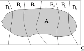
1.6.2 Law of Total Probability and Bayes’ Rule

SupposeB1, B2, . . . , Bnis apartitionof Ω. That is,B1, B2, . . . , Bnare disjoint

and their union is Ω, see Figure 1.16

A

B B2 B3 B4 B5 B

6 1

Ω

Figure 1.16: A partition of the sample space

Then, by the sum rule, P(A) =n_i₌₁P(A_∩Bi) and hence, by the definition of

conditional probability we have

P(A) =n_i₌₁P(A|Bi)P(Bi)

This is called the law of total probability.

Combining the Law of Total Probability with the definition of conditional prob-ability gives Bayes’ Rule:

P(Bj|A) = P

(A_|Bj)P(Bj)

n

i=1 P(A|Bi)P(Bi)

(29)

probability of a defective chip at 1, 2, 3 is 0.01, 0.05, 0.02, respectively. Suppose someone shows us a defective chip. What is the probability that this chip comes from factory 1?

LetBi denote the event that the chip is produced by factoryi. The{B} form

a partition of Ω. LetAdenote the event that the chip is faulty. By Bayes’ rule,

P(B1|A) =

0.15_×0.01

0.15×0.01 + 0.35×0.05 + 0.5×0.02 = 0.052.

1.6.3 Independence

Independence is a very important concept in probability and statistics. Loosely speaking it models the lack of information between events. We say A and

B are independent if the knowledge that A has occurred does not change the probability thatB occurs. That is

A,B independent_⇔P(A_|B) =P(A)

SinceP(A_|B) =P(A_∩B)/P(B) an alternative definition of independence is

A,B independent_⇔_P(A_∩B) =_P(A)_P(B)

This definition covers the caseB =∅(empty set). We can extend the definition to arbitrarily many events:

Definition 1.3 The events A1, A2, . . . , are said to be (mutually) indepen-dentif for anyn and any choice of distinct indices i1, . . . , ik,

P(Ai1 ∩Ai2∩ · · · ∩Aik) =P(Ai1)P(Ai2)· · ·P(Aik).

Remark 1.1 In most cases independence of events is a model assumption. That is, we assume that there exists a Psuch that certain events are indepen-dent.

Example 1.15 (A Coin Toss Experiment and the Binomial Law) We flip a coinntimes. We can write the sample space as the set of binary n-tuples:

Ω ={(0, . . . ,0), . . . ,(1, . . . ,1)}.

Here 0 represent Tails and 1 represents Heads. For example, the outcome (0,1,0,1, . . .) means that the first time Tails is thrown, the second time Heads, the third times Tails, the fourth time Heads, etc.

How should we defineP? LetAidenote the event of Heads during theith throw,

i= 1, . . . , n. Then,Pshould be such that the eventsA1, . . . , Anareindependent.

And, moreover,P(Ai) should be the same for alli. We don’t know whether the

(30)

These two rules completely specify P. For example, the probability that the first kthrows are Heads and the last n−kare Tails is

P({(1,1, . . . ,1,0,0, . . . ,0)}) = P(A1)· · ·P(Ak)· · ·P(Akc+1)· · ·P(Acn)

= pk(1₋p)n−k.

Also, let Bk be the event that there are k Heads in total. The probability of

this event is the sum the probabilities of elementary events {(x1, . . . , xn)}such

that x1+· · ·+xn=k. Each of these events has probabilitypk(1−p)n−k, and

there aren_k of these. Thus,

P(Bk) =

n

k p

k₍₁

−p)n−k, k= 0,1, . . . , n .

We have thus discovered thebinomial distribution.

Example 1.16 (Geometric Law) There is another important law associated with the coin flip experiment. Suppose we flip the coin until Heads appears for the first time. LetCk be the event that Heads appears for the first time at the

k-th toss, k = 1,2, . . .. Then, using the same events _{Ai} as in the previous

example, we can write

Ck =Ac1∩Ac2∩ · · · ∩Ack−1∩Ak,

so that with the product law and the mutual independence of Ac

1, . . . , Ak we

have thegeometric law:

P(Ck) =P(Ac1)· · ·P(Ack−1)P(Ak)

= (1₋p)_{· · ·}(1₋p)

k−1 times

(31)

Chapter 2

Random Variables and

Probability Distributions

Specifying a model for a random experiment via a complete description of Ω andPmay not always be convenient or necessary. In practice we are only inter-ested in variousobservations (i.e., numerical measurements) of the experiment. We include these into our modelling process via the introduction of random variables.

2.1 Random Variables

Formally arandom variableis afunctionfrom the sample space Ω to_R. Here is a concrete example.

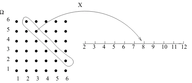
Example 2.1 (Sum of two dice) Suppose we toss two fair dice and note their sum. If we throw the dice one-by-one and observe each throw, the sample space is Ω =_{(1,1), . . . ,(6,6)_}. The functionX, defined by X(i, j) =i+j, is a random variable, which maps the outcome (i, j) to the sumi+j, as depicted in Figure 2.1. Note that all the outcomes in the “encircled” set are mapped to 8. This is the set of all outcomes whose sum is 8. A natural notation for this set is to write{X = 8}. Since this set has 5 outcomes, and all outcomes in Ω are equally likely, we have

P(_{X= 8_}) = 5 36.

This notation is very suggestive and convenient. From a non-mathematical viewpoint we can interpret X as a “random” variable. That is a variable that can take on several values, with certain probabilities. In particular it is not diﬃcult to check that

P(_{X =x_}) = 6− |7−x|

(32)

2 3 4 5 6 7 8 9 10 11 12

1 2 3 4 5 6

X

Ω

Figure 2.1: A random variable representing the sum of two dice

Although random variables are, mathematically speaking, functions, it is often convenient to view random variables as observations of a random experiment that has not yet been carried out. In other words, a random variable is consid-ered as a measurement that becomes available once we carry out the random experiment, e.g.,tomorrow. However, all thethinkingabout the experiment and measurements can be done today. For example, we can specify today exactly the probabilities pertaining to the random variables.

We usually denote random variables withcapitalletters from the last part of the alphabet, e.g. X, X1, X2, . . . , Y, Z. Random variables allow us to use natural and intuitive notations for certain events, such as {X = 10}, {X > 1000},

{max(X, Y)_≤Z_}, etc.

Example 2.2 We flip a coinntimes. In Example 1.15 we can find a probability model for this random experiment. But suppose we are not interested in the complete outcome, e.g., (0,1,0,1,1,0. . . ), but only in the total number of heads (1s). Let X be the total number of heads. X is a “random variable” in the true sense of the word: X could lie anywhere between 0 and n. What we are interested in, however, is the probability that X takes certain values. That is, we are interested in the probability distribution of X. Example 1.15 now suggests that

P(X=k) =

n

k p

k₍₁₋_p₎n−k_, _k_{= 0}_,₁_{, . . . , n .} _(2.1)

This contains all the information aboutXthat we could possibly wish to know. Example 2.1 suggests how we can justify this mathematically Define X as the function that assigns to each outcomeω= (x1, . . . , xn) the numberx1+· · ·+xn.

Then clearlyXis a random variable in mathematical terms (that is, a function). Moreover, the event that there are exactly kHeads in nthrows can be written as

{ω∈Ω :X(ω) =k}.

(33)

2.2 Probability Distribution 31

We give some more examples of random variables without specifying the sample space.

1. The number of defective transistors out of 100 inspected ones, 2. the number of bugs in a computer program,

3. the amount of rain in Brisbane in June, 4. the amount of time needed for an operation.

The set of all possible values a random variableX can take is called therange ofX. We further distinguish between discrete and continuous random variables:

Discrete random variables can only takeisolated values.

For example: a count can only take non-negative integer values. Continuous random variables can take values in an interval.

For example: rainfall measurements, lifetimes of components, lengths, . . . are (at least in principle) continuous.

2.2 Probability Distribution

LetXbe a random variable. We would like to specify the probabilities of events such as {X=x}and {a≤X≤b}.

If we can specify all probabilities involving X, we say that we have specified the probability distributionof X.

One way to specify the probability distribution is to give the probabilities of all events of the form_{X_≤x_},x_∈R. This leads to the following definition.

Definition 2.1 The cumulative distribution function (cdf) of a random variableX is the function F :R→[0,1] defined by

F(x) :=P(X_≤x), x_∈R.

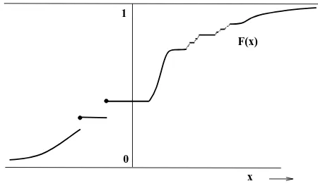
Note that above we should have written _P(_{X _≤ x_}) instead of _P(X _≤ x). From now on we will use this type of abbreviation throughout the course. In Figure 2.2 the graph of a cdf is depicted.

(34)

x F(x)

0 1

Figure 2.2: A cumulative distribution function

1. F is right-continuous: limh↓0F(x+h) =F(x), 2. limx→∞F(x) = 1; limx→−∞F(x) = 0.

3. F is increasing: x_≤y_⇒F(x)_≤F(y), 4. 0_≤F(x)_≤1.

Proof_{. We will prove (1) and (2) in STAT3004. For (3), suppose} _x _≤_y _and

define A=_{X _≤x_}and B =_{X _≤y_}. Then, obviously, A_⊂B (for example if_{X_≤3_}then this implies _{X_≤4_}). Thus, by (2) on page 14,P(A)_≤P(B), which proves (3). Property (4) follows directly from the fact that 0≤P(A)≤1 for any eventA — and hence in particular forA=_{X_≤x_}.

Any functionF with the above properties can be used to specify the distribution of a random variable X. Suppose thatX has cdf F. Then the probability that

X takes a value in the interval (a, b] (excluding a, includingb) is given by P(a < X _≤b) =F(b)₋F(a).

Namely,P(X_≤b) =P(_{X _≤a_}∪{a < X _≤b_}), where the events_{X_≤a_}and

{a < X _≤b_} are disjoint. Thus, by the sum rule: F(b) =F(a) +_P(a < X _≤b), which leads to the result above. Note however that

P(a_≤X _≤b) =F(b)₋F(a) +P(X =a) =F(b)₋F(a) +F(a)₋lim

h↓0F(a−h) =F(b)₋lim

h↓0F(a−h).

(35)

2.2 Probability Distribution 33

2.2.1 Discrete Distributions

Definition 2.2 We say that X has a discrete distribution if X is a discrete random variable. In particular, for some finite or countable set of values

x1, x2, . . . we have P(X = xi) > 0, i = 1,2, . . . and iP(X = xi) = 1. We

define the probability mass function (pmf) f of X by f(x) = P(X = x). We sometimes writefX instead off to stress that the pmf refers to the random

variableX.

The easiest way to specify the distribution of a discrete random variable is to specify its pmf. Indeed, by the sum rule, if we knowf(x) for allx, then we can calculate all possible probabilities involvingX. Namely,

P(X _∈B) =

x∈B

f(x) (2.2)

for any subsetB of the range of X.

Example 2.3 Toss a die and let X be its face value. X is discrete with range

{1,2,3,4,5,6}. If the die is fair the probability mass function is given by

Example 2.4 Toss two dice and letX be the largest face value showing. The pmf ofX can be found to satisfy

x 1 2 3 4 5 6

Definition 2.3 A random variable X is said to have a continuous distri-bution if X is a continuous random variable for which there exists apositive functionf withtotal integral 1, such that for all a, b

P(a < X ≤b) =F(b)−F(a) =

b

a

(36)

The functionf is called theprobability density function(pdf) of X.

f(x)

x

a b

Figure 2.3: Probability density function (pdf)

Note that the corresponding cdf F is simply a primitive (also called anti-derivative) of the pdf f. In particular,

F(x) =P(X _≤x) =

x

−∞

f(u)du.

Moreover, if a pdff exists, then f is thederivative of the cdf F:

f(x) = d

dxF(x) =F

′₍_x₎_.

We caninterpret f(x) as the “density” thatX =x. More precisely,

P(x_≤X_≤x+h) =

x+h

x

f(u)du_≈h f(x).

However, it is important to realise that f(x) is not a probability — is a prob-ability density. In particular, if X is a continuous random variable, then P(X =x) = 0, for all x. Note that this also justifies usingP(x≤X ≤x+h) above instead of P(x < X_≤x+h). Although we will use the same notation f

for probability mass function (in the discrete case) and probability density func-tion (in the continuous case), it is crucial to understand the diﬀerence between the two cases.

Example 2.5 Draw a random number from the interval of real numbers [0,2]. Each number is equally possible. Let X represent the number. What is the probability density functionf and the cdfF ofX?

Solution: Take an x∈[0,2]. Drawing a numberX “uniformly” in [0,2] means that P(X_≤x) =x/2, for all suchx. In particular, the cdf ofX satisfies:

F(x) =

⎧ ⎨ ⎩

0 x <0, x/2 0_≤x_≤2,

1 x >2.

By diﬀerentiatingF we find

f(x) =

1/2 0_≤x_≤2,

(37)

2.3 Expectation 35

Note that this density is constant on the interval [0,2] (and zero elsewhere), reflecting that each point in [0,2] is equally likely. Note also that we have modelled this random experiment using a continuous random variable and its pdf (and cdf). Compare this with the more “direct” model of Example 1.9.

Describing an experiment via a random variable and its pdf, pmf or cdf seems much easier than describing the experiment by giving the probability space. In fact, we have not used a probability space in the above examples.

2.3 Expectation

Although all the probability information of a random variable is contained in its cdf (or pmf for discrete random variables and pdf for continuous random variables), it is often useful to consider various numerical characteristics of that random variable. One such number is theexpectation of a random variable; it is a sort of “weighted average” of the values that X can take. Here is a more precise definition.

Definition 2.4 LetX be adiscreterandom variable with pmff. The expec-tation (or expected value) of X, denoted by EX, is defined by

EX =

x

xP(X=x) =

x

x f(x).

The expectation ofX is sometimes written as µX.

Example 2.6 FindEX ifX is the outcome of a toss of a fair die. SinceP(X= 1) =. . .=P(X= 6) = 1/6, we have

EX= 1 (1 6) + 2 (

1

6) +. . .+ 6 ( 1 6) =

7 2.

Note: EX is not necessarily a possible outcome of the random experiment as in the previous example.

One way to interpret the expectation is as a type of “expected profit”. Specifi-cally, suppose we play a game where you throw two dice, and I pay you out, in dollars, the sum of the dice,X say. However, to enter the game you must pay med dollars. You can play the game as many times as you like. What would be a “fair” amount ford? The answer is

d=_EX = 2_P(X= 2) + 3_P(X = 3) +_{· · ·}+ 12_P(X = 12) = 2 1

36 + 3 2

(38)

Namely, in the long run the fractions of times the sum is equal to 2, 3, 4, . . . are ₃₆1 ,₃₅2,₃₆3, . . ., so the average pay-out per game is the weighted sum of 2,3,4,. . . with the weights being the probabilities/fractions. Thus the game is “fair” if the average profit (pay-out - d) is zero.

Another interpretation of expectation is as acentre of mass. Imagine that point masses with weights p1, p2, . . . , pn are placed at positionsx1, x2, . . . , xn on the

real line, see Figure 2.4.

pn p2

p1

xn

EX

x1 x2

Figure 2.4: The expectation as a centre of mass

Then there centre of mass, the place where we can “balance” the weights, is centre of mass =x1p1+· · ·+xnpn,

which is exactly the expectation of the discrete variableXtaking valuesx1, . . . , xn

with probabilities p1, . . . , pn. An obvious consequence of this interpretation is

that for a symmetric probability mass function the expectation is equal to the symmetry point (provided the expectation exists). In particular, suppose

f(c+y) =f(c₋y) for all y, then

EX =c f(c) +

x>c

xf(x) +

x<c

xf(x)

=c f(c) +

y>0

(c+y)f(c+y) +

y>0

(c₋y)f(c₋y)

=c f(c) +

y>0

c f(c+y) +c

y>0

f(c−y)

=c

x

f(x) =c

For continuous random variables we can define the expectation in a similar way:

Definition 2.5 Let X be a continuous random variable with pdf f. The ex-pectation(or expected value) of X, denoted by EX, is defined by

EX=

x

x f(x)dx .

(39)

2.3 Expectation 37

entirely “obvious”: the expected value of a function ofXis the weighted average of the values that this function can take.

Theorem 2.1 IfX isdiscrete with pmff, then for any real-valued functiong

Eg(X) =

x

g(x)f(x).

Similarly, ifX iscontinuous with pdff, then

Eg(X) =

_∞

−∞

g(x)f(x)dx .

Proof_{. We prove it for the discrete case only. Let} _Y ₌_g₍_X_{), where} _X _{is a}

discrete random variable with pmffX, andgis a function. Y is again a random

variable. The pmf ofY,fY satisfies

fY(y) =P(Y =y) =P(g(X) =y) =

Thus, the expectation ofY is EY =

An important consequence of Theorem 2.1 is that the expectation is “linear”. More precisely, for any real numbersaand b, and functionsg and h

1. E(a X+b) =aEX+b .

2. E(g(X) +h(X)) =Eg(X) +Eh(X) .

Proof_{. Suppose}_X _{has pmf}_f_{. Then 1. follows (in the discrete case) from}

(40)

The continuous case is proved analogously, by replacing the sum with an inte-gral.

Another useful number about (the distribution of) X is the variance of X. This number, sometimes written as σ2_X, measures the spread or dispersion of the distribution ofX.

Definition 2.6 The variance of a random variable X, denoted by Var(X) is defined by

Var(X) =E(X−EX)2 .

The square root of the variance is called thestandard deviation. The number EXr is called therth momentof X.

The following important properties for variance hold for discrete or continu-ous random variables and follow easily from the definitions of expectation and variance.

1. Var(X) =EX2₋(EX)2 2. Var(aX +b) =a2Var(X)

Proof_{. Write} _E_X ₌ _µ_{, so that Var(}_X_{) =} _E₍_X₋_µ₎2 ₌ _E₍_X2₋₂_µX ₊_µ2_).

By the linearity of the expectation, the last expectation is equal to the sum E(X2)−2µEX+µ2 =EX2−µ2, which proves 1. To prove 2, note first that the expectation of aX+bis equal to aµ+b. Thus,

Var(aX+b) =E(aX+b₋(aµ+b))2 =E(a2(X₋µ)2) =a2Var(X).

2.4 Transforms

Many calculations and manipulations involving probability distributions are fa-cilitated by the use oftransforms. We discuss here a number of such transforms.

Definition 2.7 Let X be a non-negative and integer-valued random variable. Theprobability generating function(PGF) ofXis the functionG: [0,1]→

[0,1] defined by

G(z) :=EzX =

∞

x=0

zxP(X =x).

Example 2.8 Let X have pmff given by

f(x) = e−λ λ

x

(41)

2.4 Transforms 39

We will shortly introduce this as the Poisson distribution, but for now this is not important. The PGF ofX is given by

G(z) =

Knowing only the PGF ofX, we can easily obtain the pmf:

P(X=x) = 1

Thus we have theuniqueness property: two pmf’s are the same if and only if their PGFs are the same.

Another useful property of the PGF is that we can obtain the moments ofX

by diﬀerentiatingGand evaluating it at z= 1. Diﬀerentiating G(z) w.r.t.z gives

G′(z) = dEz

Et cetera. If you’re not convinced, write out the expectation as a sum, and use the fact that the derivative of the sum is equal to the sum of the derivatives (although we need a little care when dealing with infinite sums).

In particular,

EX =G′(1),

and

(42)

Definition 2.8 Themoment generating function(MGF) of a random vari-able X is the function,M :I →[0,∞), given by

M(s) =EesX .

Here I is an open interval containing 0 for which the above integrals are well defined for alls_∈I.

In particular, for a discrete random variable with pmf f,

M(s) =

x

esxf(x),

and for a continuous random variable with pdff,

M(s) =

x

esxf(x)dx .

We sometimes write MX to stress the role of X.

As for the PGF, the moment generation function has theuniqueness property: Two MGFs are the same if and only if their corresponding distribution functions are the same.

Similar to the PGF, the moments of X follow from the derivatives ofM: If EXn _{exists, then} _M _is _n_{times diﬀerentiable, and}

EXn=M(n)(0).

Hence the name moment generating function: the moments of X are simply found by diﬀerentiating. As a consequence, the variance ofX is found as

Var(X) =M′′(0)₋(M′(0))2.

Remark 2.1 The transforms discussed here are particularly useful when deal-ing with sums of independent random variables. We will return to them in Chapters 4 and 5.

2.5 Some Important Discrete Distributions

In this section we give a number of important discrete distributions and list some of their properties. Note that the pmf of each of these distributions depends on one or more parameters; so in fact we are dealing withfamiliesof distributions.

2.5.1 Bernoulli Distribution

We say that X has a Bernoulli distribution with success probability p if X

(43)

2.5 Some Important Discrete Distributions 41

We writeX_∼Ber(p). Despite its simplicity, this is one of the most important distributions in probability! It models for example a single coin toss experiment. The cdf is given in Figure 2.5.

1−p 1

0 1

Figure 2.5: The cdf of the Bernoulli distribution

Here are some properties:

1. The expectation isEX = 0P(X = 0)+1P(X = 1) = 0_×(1₋p)+1_×p=p. 2. The variance is Var(X) =EX2−(EX)2 =EX−(EX)2 =p−p2=p(1−p).

(Note that X2₌_X_).

3. The PGF is given byG(z) =z0(1₋p) +z1p= 1₋p+zp.

2.5.2 Binomial Distribution

Consider a sequence ofncoin tosses. IfX is the random variable which counts the total number of heads and the probability of “head” is p then we say X

has abinomialdistribution with parametersnandpand writeX∼Bin(n, p). The probability mass functionX is given by

f(x) =P(X =x) =

n x p

x₍₁₋_p₎n−x_, _x_{= 0}_,₁_{, . . . , n.} _(2.4)

This follows from Examples 1.15 and 2.2. An example of the graph of the pmf is given in Figure 2.6

Here are some important properties of the Bernoulli distribution. Some of these properties can be proved more easily after we have discussed multiple random variables.

1. The expectation is EX = np. This is a quite intuitive result. The ex-pected number of successes (heads) inncoin tosses isnp, ifpdenotes the probability of success in any one toss. To prove this, one could simply evaluate the sum

n

x=0

x

n x p

x₍₁₋_p₎n−x_,

(44)

0 1 2 3 4 5 6 7 8 9 10

Figure 2.6: The pmf of theBin(10,0.7)-distribution

whereXi indicates whether thei-th toss is a success or not,i= 1, . . . , n.

Also we will prove that the expectation of such a sum is the sum of the expectation, therefore,

we can easily prove this after we consider multiple random variables in Chapter 4. Namely,

G(z) =EzX =EzX1+···+Xn ₌_E_zX1_{· · ·}_E_zXn

= (1−p+zp)× · · · ×(1−p+zp) = (1−p+zp)n .

However, we can also easily prove it using Newton’s binomial formula:

(a+b)n=

Note that once we have obtained the PGF, we can obtain the expectation and variance as G′(1) =npand G′′(1) +G′(1)₋(G′(1))2 = (n₋1)np2+

(45)

2.5.3 Geometric distribution

Again we look at a sequence of coin tosses but count a diﬀerent thing. LetX

be the number of tosses needed before the first head occurs. Then

P(X=x) = (1₋p)x−1p, x= 1,2,3, . . . (2.5) since the only string that has the required form is

ttt . . . t

x−1

h

and this has probability (1−p)x−1p.See also Example 1.16 on page 28. Such a random variableX is said to have a geometricdistribution with parameterp. We writeX_∼G(p). An example of the graph of the pdf is given in Figure 2.7

1 2 3 4 5 6 7 8 9 10 11 12 13 14 15 16 0.05

0.1 0.15 0.2 0.25 0.3

p=0.3

Figure 2.7: The pmf of theG(0.3)-distribution

We give some more properties, including the expectation, variance and PGF of the geometric distribution. It is easiest to start with the PGF:

1. The PGF is given by

G(z) =

∞

x=1

zxp(1₋p)x−1=z p

∞

k=0

(z(1₋p))k = z p 1₋z(1₋p),

using the well-known result for geometric sums: 1 +a+a2+_{· · ·} = ₁₋1_a, for_|a_|<1.

2. The expectation is therefore

EX=G′(1) = 1

p,

(46)

3. By diﬀerentiating the PGF twice we find the variance:

Var(X) =G′′(1) +G′(1)−(G′′(1))2 = 2(1−p)

p2 +

1

p−

1

p2 = 1₋p

p2 .

4. The probability of requiring more than ktosses before a success is P(X > k) = (1₋p)k.

This is obvious from the fact that{X > k}corresponds to the event of k

consecutive failures.

A final property of the geometric distribution which deserves extra attention is thememoryless property. Think again of the coin toss experiment. Suppose we have tossed the coinktimes without a success (Heads). What is the proba-bility that we need more thanx additional tosses before getting a success. The answer is, obviously, the same as the probability that we require more than x

tosses if we start from scratch, that is, P(X > x) = (1₋p)x, irrespective ofk. The fact that we have already hadkfailures does not make the event of getting a success in the next trial(s) any more likely. In other words, the coin does not have a memory of what happened, hence the word memoryless property. Mathematically, it means that for anyx, k = 1,2, . . .,

P(X > k+x|X > k) =P(X > x)

Proof_{. By the definition of conditional probability}

P(X > k+x_|X > k) = P({X=k+x} ∩ {X > k}) P(X > k) .

Now, the event {X > k+x} is a subset of {X > k}, hence their intersection is _{X > k+x_}. Moreover, the probabilities of the events _{X > k+x_} and

{X > k_} are (1₋p)k+x _{and (1}₋_p₎k_{, respectively, so that}

P(X > k+x_|X > k) = (1−p)

k+x

(1−p)k = (1−p)

x ₌_P₍_{X > x}₎_,

as required.

2.5.4 Poisson Distribution

A random variableX for which

P(X=x) = λ

x

x! e

−λ_, _x_{= 0}_,₁_,₂_{, . . . ,} _(2.6)

(47)

coin tossing experiment where we toss a coin ntimes with success probability

λ/n. LetXbe the number of successes. Then, as we have seenX ∼Bin(n, λ/n). e−λ _{(this is one of the defining properties of the exponential function). Hence,}

we have

which shows that the Poisson distribution is a limiting case of the binomial one. An example of the graph of its pmf is given in Figure 2.8

0 1 2 3 4 5 6 7 8 9 1011121314151617181920

Figure 2.8: The pdf of thePoi(10)-distribution

We finish with some properties.

1. The PGF was derived in Example 2.8:

G(z) = e−λ(1−z) .

2. It follows that the expectation isEX =G′(1) =λ. The intuitive explana-tion is that the mean number of successes of the corresponding coin flip experiment is np=n(λ/n) =λ.

3. The above argument suggests that the variance should be n(λ/n)(1₋

λ/n)→λ. This is indeed the case, as

Var(X) =G′′(1) +G′(1)₋(G′(1))2 =λ2+λ₋λ2=λ .

(48)

2.5.5 Hypergeometric Distribution

We say that a random variable X has aHypergeometric distribution with parameters N,nand r if

P(X=k) =

_r

k

_N₋_r

n−k

_N

n

,

for max_{0, r+n₋N_{} ≤}k_≤min_{n, r_}.

We write X _∼ Hyp(n, r, N). The hypergeometric distribution is used in the following situation.

Consider an urn withN balls, r of which are red. We draw at randomnballs from the urn without replacement. The number of red balls amongst the n

chosen balls has aHyp(n, r, N) distribution. Namely, if we number the red balls 1, . . . , rand the remaining ballsr+1, . . . , N, then the total number of outcomes of the random experiment isN_n, and each of these outcomes is equally likely. The number of outcomes in the event “k balls are red” is _kr×N_n₋−_kr because thekballs have to be drawn from ther red balls, and the remainingn₋kballs have to be drawn from the N₋knon-red balls. In table form we have:

Red Not Red Total

Selected k n−k n

Not Selected r−k N−n−r+k N−n

Total r N ₋r N

Example 2.9 Five cards are selected from a full deck of 52 cards. Let X be the number of Aces. ThenX _∼Hyp(n= 5, r= 4, N = 52).

k 0 1 2 3 4

P(X=k) 0.659 0.299 0.040 0.002 0.000 1

The expectation and variance of the hypergeometric distribution are EX=n r

N

and

Var(X) =n r N

1₋ r

N

_N₋_n

N−1 .

(49)

2.6 Some Important Continuous Distributions 47

2.6 Some Important Continuous Distributions

In this section we give a number of important continuous distributions and list some of their properties. Note that the pdf of each of these distributions depends on one or more parameters; so, as in the discrete case discussed before, we are dealing withfamiliesof distributions.

2.6.1 Uniform Distribution

We say that a random variable X has a uniform distribution on the interval [a, b], if it has density function f, given by

f(x) = 1

b−a, a≤x≤b .

We write X ∼U[a, b]. X can model a randomly chosen point from the inter-val [a, b], where each choice is equally likely. A graph of the pdf is given in Figure 2.9.

a b

1

b−a

x_→

Figure 2.9: The pdf of the uniform distribution on [a, b]

We have

This can be seen more directly by observing that the pdf is symmetric around

c= (a+b)/2, and that the expectation is therefore equal to the symmetry point

c. For the variance we have

Var(X) =EX2₋(EX)2 =

(50)

2.6.2 Exponential Distribution

A random variableX with probability density functionf, given by

f(x) =λe−λ x, x_≥0 (2.7) is said to have an exponentialdistribution with parameterλ. We writeX ∼

Exp(λ). The exponential distribution can be viewed as a continuous version of the geometric distribution. Graphs of the pdf for various values of λare given in Figure 2.10.

Figure 2.10: The pdf of theExp(λ)-distribution for variousλ(c should beλ).

Here are some properties of the exponential function:

1. The moment generating function is

M(s) =

2. From the moment generating function we find by diﬀerentiation:

EX=M′(0) = λ

Alternatively, you can use partial integration to evaluate