Generalized Space-Time
Autoregressive Modeling
Dhoriva Urwatul Wutsqa1, Suhartono2 and Brodjol Sutijo2
1Department of Mathematics Education, University of State Yogyakarta, Indonesia
2Department of Statistics, Institute Technology of Sepuluh Nopember, Indonesia
Abstract. Generalized Space-Time Autoregressive (GSTAR) model is relatively new method for spatial time series data. It is a generalization of Space-Time Autoregressive (STAR) model that allows the autoregressive parameters vary in each location. In this paper we discuss the procedure to build the GSTAR model. The steps are similar to those of Box-Jenkins procedure, starting from order selection of spatial and temporal autoregressive model, parameters estimation, and diagnostic check of white noise errors. The Akaike’s Information Criterion (AIC) is used for order selection. Particularly, there are two types estimation in GSTAR model. The first is determining space weights; here we propose normalization of cross-correlation between locations. The second is estimating the autoregressive parameters, which is performed by using least square method. We develop Wald test for evaluating the significance of the least square estimators. The Pormanteau multivariate test is adopted for detecting white noise error in multivariate case. Simulation study is performed to all the steps to illustrate the computation of the procedure.
Keywords:
GSTAR Modeling, Akaike’s Information Criteria, normalization of cross-correlation,Wald test, Pormanteau multivariate test
1 Introduction
Spatial time series is addressed to the data that depend on time and site. It deals with single variable observed over time at a number of different locations. Daily air pollution measurements recorded from detector at many location, daily oil production at a number of wells, and traffic flow measurements taken from a set of loop detectors in a very frequent basis are examples of spatial time series data. Such kinds of data are also recognized as space time data.
parameters than VARMA model. Then, Pfeifer dan Deutsch [6,7] further studied those models and developed the procedure of their modeling
In STAR model, the autoregressive parameters are assumed to be the same for all locations. This assumption is impractical, since different locations usually lead different parameters. A more flexible model, i.e., Generalized STAR model was proposed by Borovkova et.al [2], allowing different autoregressive parameters.
This paper present the method of GSTAR modeling through the procedures adopted from Box and Jenkins [1]. The procedures start from stationer condition. Discussions about stationery GSTAR model can be read extensively in [8,9] and [12]. This paper focuses the discussion on the three stage modeling procedure. Those are model identification, parameters estimation, and diagnostic check to ensure that the model has white noise error vector.
2. GSTAR (Generalized Space-Time Autoregressive) Model
The GSTAR model is specific form of VAR (Vector Autoregressive)
model. It reveals linear dependencies of space and time. The main difference is
on the spatial dependent, that in GSTAR model, it is expressed by weight
matrix. Let
{
Z t( ) :t= ± ±0, 1, 2,...}
be a multivariate time series of Ncomponents. In matrix notation, the GSTAR model of autoregressive order p
and spatial orders λ1λ2,...,λp, GSTAR (pλ1λ2,...,λp) could be written as (see [2])
( ) 0
1 1
( )
(
)
( )
s p
k
s sk
s k
Z t
W
Z t
s
e t
λ
= =
⎡
⎤
=
⎢
Φ + Φ
⎥
− +
⎣
⎦
∑
∑
(1)where
(
1 N)
0 diag s0, , s0
s φ φ
Φ = … and
(
1 N)
sk sk
diag , ,
sk φ φ
Φ = … ,
weights are choosen to satisfy
w
ii( )k=
0
and ij( )k 1 i j≠ w =3. Model Identification
As in time series modeling, the first step is identifying a tentative model
which is characterized by spatial and time order. Spatial order is generally
restricted on order 1, since the higher order is difficult to be interpreted.
Approving the method in VAR and VARMA models, the time (autoregressive)
order is determined by using the Akaike Information Criterion (AIC) (see
[13])
AIC(i) =
( )
2
2 ˆ ln
T i
k i
Σ + (2)
where k is the number of parameters in the model and T is the number of
observation. The autoregressive order of GSTAR model is p such that
AIC(p) =
0
0
min ≤ ≤i p AIC( )i . This value p can be obtained by performing SAS
program using PROCSTATESPACE.
4. Parameters Estimation
4.1 Determination of space weight
Determination of space weight by using the normalisation result of
cross-correlation between locations at the appropriate time lag is firstly proposed by
the method well performed on GSTAR(11) model. In general, cross-correlation
between two variables or location i and j at the time lag k, corr[Zi(t),Zj(t−k)],
defined as (see [1, 14])
( ) ( ),
j i ij ij
k k
σ σ γ
ρ = k=0,±1 ,±2,… (3)
where γij(k) is cross-covarians between observation in location i and j at the
time lag k, σi and σj is standard deviation of observation in location i and j.
The estimated of cross-correlation in sample data is
⎟⎟⎠ ⎞ ⎜⎜⎝
⎛ −
⎟⎟⎠ ⎞ ⎜⎜⎝
⎛ −
− − −
=
∑ ∑
∑
= =
+ =
n
t
j j n
t
i i n
k t
j j
i i
ij
Z t Z Z
t Z
Z k t Z Z t Z k
r
1
2 1
2 1
] ) ( [ ] ) ( [
] ) ( ][ ) ( [ )
( . (4)
Then, determination of space weight could be done by normalisation of the
the cross-correlation between locations at the appropriate time lag. This
process generally yields space weight for GSTAR(p1) model, i.e.
( ) , | ( ) |
ij ij
ik k i
r k w
r k
≠
=
∑
where i≠ j, k = 1, …, p (5)and this weight satisfies | | 1 1
=
∑
≠ j
ij
w
Space weights by using the normalisation of the cross-correlation between
relationship between locations. Hence, there is no strict constraint about the
weight values that must depend on distance between locations. This weight
also gives flexibility on the sign and size of the relationship between locations.
4.2. Autoregressive Parameter Estimation of GSTAR (pλ1λ2,...,λp) model
Recall GSTAR (pλ1λ2,...,λp) model
(
)
( ) ( ) ( ) ( )
1 1 2 2
1 0
( ) ( ) ( ) ( ) ( )
s p
i k k k
i sk i i iN N i
s k
Z t w Z t s w Z t s w Z t s t
λ
ϕ
= =
=
∑∑
− + − + + − +e (6)for t= p p, +1,...,T, i = 1, 2, ..., N, where (0) 1
ij
w = for i = j and zero otherwise.
It is assumed that e( )t ∼White Noise (0, ∑) , where e(t) = (e t ,1( ) e t , …, 2( )
( ) N
e t )
Least square estimator of autoregressive parameter has been dirived by
Borovkova et.al [3]. They define new notations
( ) ( )
( ) ( )
N
k k
i ij j
j i
V t w Z t
≠
=
∑
for k ≥ 1 and (0)( ) ( )i i
V t =Z t ,
(
( ),..., ( ))
i = Z pi Z Ti ′
Y , ui =
(
e pi( ),..., ( )e Ti)
′1 1
1 1
( ) ( )
(0) (0)
( ) ( )
(0) (0)
( 1) ( 1) (0) (0)
( 1) ( 1) ( ) ( )
p
p
i i i i
i
i i i i
V p V p V V
V T V T V T p V T p
λ λ
λ λ
⎛ − − ⎞
⎜ ⎟
= ⎜ ⎟
⎜ − − − − ⎟
⎝ ⎠
and
(
)
1 2
( ) ( ) ( ) ( ) ( ) ( ) 10 ,..., 1 , 20,..., 2 ,..., 0,..., p
i i i i i i
i = φ φ φλ φλ φp φλ ′
β
Equation (6) can be expressed for all location simultaneously as linear model = +
Y Xβ u, (7)
where Y=
(
Y1′,...,YN′)
′, X=(
X1,...,XN)
, β=(
β1′,...,βN′)
′, u=(
u1′,...,u′N)
′Thus, least square estimator ˆβTis of the form
βˆT =
( )
X X′ −1X u′ (8)Asymptotic normality of the estimator ˆβT will be explained below.
Write M =diag
(
M1,...,MN)
where Mi =diag(
Mi1,...,Mip)
, for i = 1, 2, ... ,N and s = 1, 2, ..., p
(1) (1) (1) (1)
1 , 1 , 1 ,
( ) ( ) ( ) ( )
1 , 1 , 1
0 0 1 0 0
0
0
s s s s
i i i i i i N
is
i i i i i iN
w w w w
w w w w
− +
− +
⎛ ⎞
⎜ ⎟
⎜ ⎟
= ⎜ ⎟
⎜ ⎟
⎜ ⎟
⎝ ⎠
M
λ λ λ λ
(9)
Define covariance matrix
( )
(0) ( 1) ( 1)
(1) (0) ( 2)
( 1) ( 2) (0)
p
p
p
p p
− − +
⎡ ⎤
⎢ − + ⎥
⎢ ⎥
= ⎢ ⎥
⎢ − − ⎥
⎣ ⎦
Γ Γ Γ
Γ Γ Γ
Γ
Γ Γ Γ
where Γ( )s = E
[
Z( )t Z′(t+s)]
.Under some conditions Borovkova et.al. [3] have shown asymptotic
multivariate normality of least square estimator in GSTAR model, i.e.
T(βˆT −β) ⎯⎯→d d( ,0 C*) (11)
where d = d = + + +(p λ1 λp)N, and
(
)
(
)
1(
)
(
(
)
)
1* = ⊗ ( )p ′ − ⊗ ( )p ′ ⊗ ( )p ′ −
C M I Γ M M ∑ Γ M M I Γ M ,
M is defined in (9) and Γ( )p is defined in (10).
The parameter ∑can be estimated by
(
)(
)
1
ˆ ( ) ˆ( ) ( ) ˆ( )
1 T
T
t p
t t t t
T p =
′
= − −
− +
∑
Z Z Z Z∑
where
( ) 0
1 1
ˆ( ) p ˆ ( ) s ˆ k ( )
s sk
s k
t =
∑
= t− +s∑
λ= t−sZ Φ Z Φ W Z
The elements of matrix Γ( )p can be estimated
0
1
ˆ ( ) ( ) ( )
1 T s
T
t
s t t s
T s
−
= ′
= − +
∑
−Γ Z Z
It is also proven in [3] that ˆ∑T dan Γˆ( )p are consistent estimators for ∑ and
( )p
Γ respectively.
The hypothesis to test the significantcy of parameter in GSTAR model can
be written as
H0 : Rβ=r against H1 : Rβ≠r. (12)
By using property (11) and the facts that ˆ∑T dan Γˆ( )p are consistent estimators
for ∑ and Γ( )p , and modifying Wald Statistic on linear model from White [15]
we develope Wald satistic for the hypothesis (12) .Let m = rank (R), if H0 :
r =
Rβ holds, under some conditions,
i) T(RβˆT −r) ( , )⎯⎯→d d 0 (13)
where d = d = + + +(p λ1 λp)N, and
=RC R* ′
ii) The Wald statistic
W=T(RβˆT −r) ( ) (′ ˆ −1 RβˆT −r) ⎯⎯→χd 2m (14)
where ˆ=RC Rˆ* ′
After found the significant model, the final step is checking wether the
model fulfill the assumtion of white noise error vector. White noise meants
residuals of model form an uncorrelated sequence that leads model fit. Based
on the estimated model, the error estimate can be written as
ˆ ˆ= ( )t ( )t
e Z - Z ,
The Portmanteau Multivariat test, a generalization of Ljung and Box (in
[13])for multivariate case, can be used to test white noise error vector. The
null hypothesis of this test is
H0 : ρ1 = = ρm =0, (15)
where ρ is correlation matrix of error vector.
The test statistic is
(
)
2 1 1
0 0 1
1 ˆ ˆ ˆ ˆ
( ) m
N t t
t
Q m T tr
T t
− −
= ′
=
−
∑
Γ Γ Γ Γ (16)Under the null hypothesis (15), the statistic test (16) approximate Chi Square
distribution with N2m degree of freedem.
6. Empirical Study
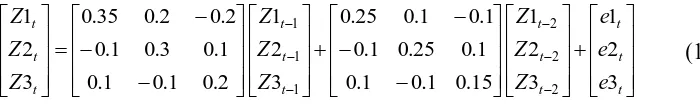
The empirical study is carried out through the simmulation study. It aims
to explain the implementation of GSTAR modeling procedures that conducted
based on the theory discribed obove. Here, the GSTAR model of spatial order
SAS program. The simulation is done for sample size 100. The simmulation
model is in the following expression
⎥ ⎥ ⎥ ⎦ ⎤ ⎢ ⎢ ⎢ ⎣ ⎡ + ⎥ ⎥ ⎥ ⎦ ⎤ ⎢ ⎢ ⎢ ⎣ ⎡ ⎥ ⎥ ⎥ ⎦ ⎤ ⎢ ⎢ ⎢ ⎣ ⎡ − − − + ⎥ ⎥ ⎥ ⎦ ⎤ ⎢ ⎢ ⎢ ⎣ ⎡ ⎥ ⎥ ⎥ ⎦ ⎤ ⎢ ⎢ ⎢ ⎣ ⎡ − − − = ⎥ ⎥ ⎥ ⎦ ⎤ ⎢ ⎢ ⎢ ⎣ ⎡ − − − − − − t t t t t t t t t t t t e e e Z Z Z Z Z Z Z Z Z 3 2 1 3 2 1 15 . 0 1 . 0 1 . 0 1 . 0 25 . 0 1 . 0 1 . 0 1 . 0 25 . 0 3 2 1 2 . 0 1 . 0 1 . 0 1 . 0 3 . 0 1 . 0 2 . 0 2 . 0 35 . 0 3 2 1 2 2 2 1 1 1 (17)
As mentioned in Section 3 the spatial order 1 is used to build GSTAR
model. And after running the simmulation data by using PROCSTATESPACE,
the minimum AIC value is in lag 2, so the autoregressive order 2 is the best
choise The result of cross-correlation between locations at the time lag 1 and 2,
) 1 (
ij
r and rij(2)where i≠ jof simulation data followed equation (4) can be
[image:10.612.135.485.172.224.2]seen in Table 1.
Tabel 1.The result of cross-correlation between locations
Parameter Coefficient estimated
The weights are attained by normalize that cross correlation using (5), i.e. ⎥ ⎥ ⎥ ⎦ ⎤ ⎢ ⎢ ⎢ ⎣ ⎡ = ⎥ ⎥ ⎥ ⎦ ⎤ ⎢ ⎢ ⎢ ⎣ ⎡ − − = 0 597 . 0 403 . 0 925 , 0 0 075 , 0 050 . 0 950 . 0 0 dan 0 826 . 0 174 . 0 772 , 0 0 228 , 0 122 . 0 878 . 0 0 2 1 W W
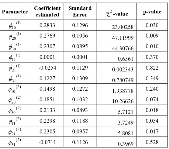
By using these weight, the resulted parameter estimates and significant test of
GSTAR(21) model are shown in Table 2.
Tabel 2. The result of parameter estimates GSTAR(21) model
Parameter Coefficient estimated Standard Error χ2
-value p-value
) 1 ( 10
φ 0.2833 0.1296 23.00258 0.030 )
1 ( 20
φ 0.2769 0.1056 47.11999 0.009 )
1 ( 30
φ 0.2307 0.0895 44.30766 0.010 )
1 ( 11
φ 0.0001 0.0001 0.6561 0.370 )
1 ( 21
φ -0.0254 0.1129 0.002343 0.822 )
1 ( 31
φ 0.1227 0.1309 0.780749 0.349 )
2 ( 10
φ 0.1498 0.1272 1.938778 0.240 )
2 ( 20
φ 0.1851 0.1032 10.26626 0.074 )
2 ( 30
φ 0.2133 0.0893 5.7121 0.018 )
2 ( 11
φ 0.2298 0.1188 3.7249 0.054 )
2 ( 21
φ 0.2305 0.0957 5.8081 0.017 )
2 ( 31
φ -0.0711 0.1126 0.3969 0.528
The last column in Table 2. reveals that not all parameters are significant.
Then, the model re-estimated after excluding the insignificant parameters one
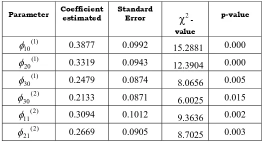
by one. The final result only includes the significant parameters, and it is
[image:11.612.176.454.276.520.2]Tabel 3.The result of significant parameter estimates GSTAR(21) model
Parameter Coefficient estimated Standard Error χ2
-value p-value ) 1 ( 10
φ 0.3877 0.0992 15.2881 0.000 )
1 ( 20
φ 0.3319 0.0943 12.3904 0.000 )
1 ( 30
φ 0.2479 0.0874 8.0656 0.005 )
2 ( 30
φ 0.2133 0.0871 6.0025 0.015 )
2 ( 11
φ 0.3094 0.1012 9.3636 0.002 )
2 ( 21
φ 0.2669 0.0905 8.7025 0.003
By using that result and applying matrix operation, the GSTAR (21) model is:
⎥ ⎥ ⎥ ⎦ ⎤ ⎢ ⎢ ⎢ ⎣ ⎡ + ⎥ ⎥ ⎥ ⎦ ⎤ ⎢ ⎢ ⎢ ⎣ ⎡ ⎥ ⎥ ⎥ ⎦ ⎤ ⎢ ⎢ ⎢ ⎣ ⎡ + ⎥ ⎥ ⎥ ⎦ ⎤ ⎢ ⎢ ⎢ ⎣ ⎡ ⎥ ⎥ ⎥ ⎦ ⎤ ⎢ ⎢ ⎢ ⎣ ⎡ = ⎥ ⎥ ⎥ ⎦ ⎤ ⎢ ⎢ ⎢ ⎣ ⎡ − − − − − − t t t t t t t t t t t t e e e Z Z Z Z Z Z Z Z Z 3 2 1 3 2 1 2133 . 0 0 0 2469 . 0 0 0200 . 0 0155 . 0 2939 . 0 0 3 2 1 2479 . 0 0 0 0 3319 . 0 0 0 0 3877 . 0 3 2 1 2 2 2 1 1 1 (18)
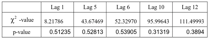
Then, the procedure continues to the last step, that is checking the white noise
assumption. Table 4. gives the result of Portmanteau Multivariate test using
Tabel 4. The result of Portmanteau Multivariate Test
It can be perceived from the p-value that the model is suitable for the white
noise error vector assumption. Thus, how to proceed all the steps of GSTAR
modeling as an implementation of theorycal result has illustrated clearly.
7. Conclusion
The method of GSTAR modeling is applyed through the procedures in the spirit of Box-Jenkins. The procedure starts from model identification involving spatial and autoregressive orders determination. Only spatial order 1 is considered, while autoregressive order is specified by minumum value of AIC (2). Normalizes cross corelation (5) is proposed as estimator of space weight and least square estimator (8) is derived as an estimate of autoregressive parameter. Wald test statistic (14) is constructed to select the significant autoregressive parameter. The Portmanteau Multivariat test (16) is cosedered as a tool to check the white noise error assumption in multivariate case. Simmulation study has been performed to describe the procedures of GSTAR modeling. As a remark on space weight determination, other technic could be attempted to obtain better estimates.
References
1. Box, G.E.P., Jenkins, G.M. and Reinsel, G.C.: Time Series Analysis, Forecasting and Control. 3rd edition, Englewood Cliffs: Prentice Hall. (1994)
2. Borovkova, S.A., Lopuhaa, H.P., and Nurani, B.: Generalized STAR model with experimental weights. In M Stasinopoulos & G Touloumi (Eds.), Proceedings of the 17th International Workshop
on Statistical Modeling (pp. 139-147). (2002)
3. Borovkova, S.A., Lopuhaa, H.P., and Nurani, B.: .Consistency and asymptotic normality of least squares estimators in generalized STAR models.Working paper. (2008)
Lag 1 Lag 5 Lag 6 Lag 10 Lag 12
2
4. Cliff. A.D., Ord, J.: Spatial Autocorrelation. London. Pioneer. (1973)
5. Lopuhaa H.P. and Borovkova S.: Asymptotic properties of least squares estimators in generalized STAR models. Technical Report. Delft University of Technology. (2005)
6. Pfeifer, P.E. and Deutsch, S.J.: A Three Stage Iterative Procedure for Space-Time Modeling.
Technometrics, Vol. 22, No. 1, pp. 35-47. (1980)
7. Pfeifer, P.E. and Deutsch, S.J.: Identification and Interpretation of First Order Space-Time ARMA Models. Technometrics, Vol. 22, No. 1, pp. 397-408. (1980)
8. Ruchjana, B.N.: Suatu Model Generalisasi Space-Time Autoregressive dan Penerapannya pada Produksi Minyak Bumi. (Disertasi, Institut Teknologi Bandung). (2002.)
9. Ruchjana, B.N.: Pemodelan Kurva Produksi Minyak Bumi Menggunakan Model Generalisasi S-TAR.
Forum Statistika dan Komputasi, IPB, Bogor. (2002).
10. Suhartono dan Atok, R.M.: Pemilihan bobot lokasi yang optimal pada model GSTAR. Prosiding
Konferensi Nasional Matematika XIII, Universitas Negeri Semarang. (2006)
11.Suhartono and Subanar.: The Optimal Determination of Space Weight in GSTAR Model by using Cross-correlation Inference. JOURNAL OF QUANTITATIVE METHODS: Journal Devoted to The
Mathematical and Statistical Application in Various Fields, Vol. 2, No. 2, pp. 45-53. (2006)
12.Suhartono and Subanar.: Some Comments on the Theorem Providing Stationarity Condition for GSTAR Models in the Paper by Borovkova et al. Journal of The Indonesian Mathematical Society (MIHMI), Vol. 13, No. 1, pp. 44-52. (2007)
13.Tsay, R.S.: Analysis of Financial Time series. John Wiley & Sons. New Jersey. (2005)
14.Wei, W.W.S.: Time series Analysis: Univariate and Multivariate Methods. Addison-Wesley Publishing Co., USA. (1990)