Copyright c2006 S. Dasgupta, C. H. Papadimitriou, and U. V. Vazirani
Contents
Preface 9
0 Prologue 11
0.1 Books and algorithms . . . 11
0.2 Enter Fibonacci . . . 12
0.3 Big-O notation . . . 15
Exercises . . . 18
1 Algorithms with numbers 21 1.1 Basic arithmetic . . . 21
1.2 Modular arithmetic . . . 25
1.3 Primality testing . . . 33
1.4 Cryptography . . . 39
1.5 Universal hashing . . . 43
Exercises . . . 48
Randomized algorithms: a virtual chapter 39 2 Divide-and-conquer algorithms 55 2.1 Multiplication . . . 55
2.2 Recurrence relations . . . 58
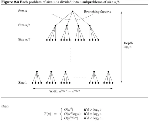
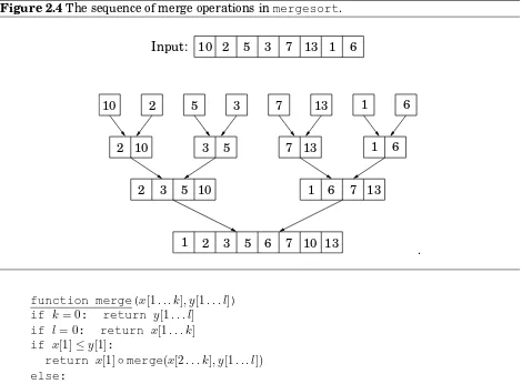
2.3 Mergesort . . . 60
2.4 Medians . . . 64
2.5 Matrix multiplication . . . 66
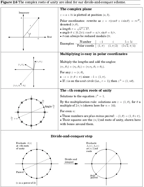
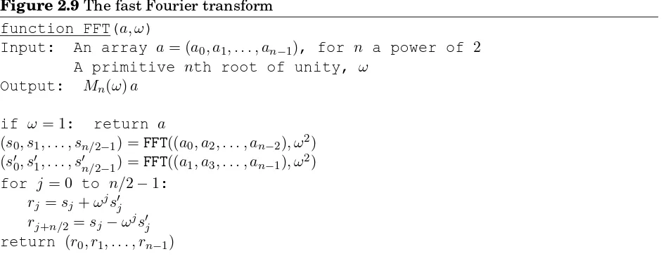
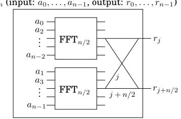
2.6 The fast Fourier transform . . . 68
Exercises . . . 83
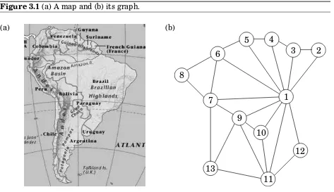
3 Decompositions of graphs 91 3.1 Why graphs? . . . 91
3.2 Depth-first search in undirected graphs . . . 93
3.3 Depth-first search in directed graphs . . . 98
3.4 Strongly connected components . . . 101
4 Paths in graphs 115
4.1 Distances . . . 115
4.2 Breadth-first search . . . 116
4.3 Lengths on edges . . . 118
4.4 Dijkstra’s algorithm . . . 119
4.5 Priority queue implementations . . . 126
4.6 Shortest paths in the presence of negative edges . . . 128
4.7 Shortest paths in dags . . . 130
Exercises . . . 132
5 Greedy algorithms 139 5.1 Minimum spanning trees . . . 139
5.2 Huffman encoding . . . 153
5.3 Horn formulas . . . 157
5.4 Set cover . . . 158
Exercises . . . 161
6 Dynamic programming 169 6.1 Shortest paths in dags, revisited . . . 169
6.2 Longest increasing subsequences . . . 170
6.3 Edit distance . . . 174
6.4 Knapsack . . . 181
6.5 Chain matrix multiplication . . . 184
6.6 Shortest paths . . . 186
6.7 Independent sets in trees . . . 189
Exercises . . . 191
7 Linear programming and reductions 201 7.1 An introduction to linear programming . . . 201
7.2 Flows in networks . . . 211
7.3 Bipartite matching . . . 219
7.4 Duality . . . 220
7.5 Zero-sum games . . . 224
7.6 The simplex algorithm . . . 227
7.7 Postscript: circuit evaluation . . . 236
Exercises . . . 239
8 NP-complete problems 247 8.1 Search problems . . . 247
8.2 NP-complete problems . . . 257
8.3 The reductions . . . 262
9 Coping with NP-completeness 283
9.1 Intelligent exhaustive search . . . 284
9.2 Approximation algorithms . . . 290
9.3 Local search heuristics . . . 297
Exercises . . . 306
10 Quantum algorithms 311 10.1 Qubits, superposition, and measurement . . . 311
10.2 The plan . . . 315
10.3 The quantum Fourier transform . . . 316
10.4 Periodicity . . . 318
10.5 Quantum circuits . . . 321
10.6 Factoring as periodicity . . . 324
10.7 The quantum algorithm for factoring . . . 326
Exercises . . . 329
Historical notes and further reading 331
List of boxes
Bases and logs . . . 21
Two’s complement . . . 27
Is your social security number a prime? . . . 33
Hey, that was group theory! . . . 36
Carmichael numbers . . . 37
Randomized algorithms: a virtual chapter . . . 39
An application of number theory? . . . 40
Binary search . . . 60
Annlognlower bound for sorting . . . 62
The Unixsortcommand . . . 66
Why multiply polynomials? . . . 68
The slow spread of a fast algorithm . . . 82
How big is your graph? . . . 93
Crawling fast . . . 105
Which heap is best? . . . 125
Trees . . . 140
A randomized algorithm for minimum cut . . . 150
Entropy . . . 155
Recursion? No, thanks. . . 173
Programming? . . . 173
Common subproblems . . . 177
Of mice and men . . . 179
Memoization . . . 183
On time and memory . . . 189
A magic trick called duality . . . 205
Reductions . . . 209
Matrix-vector notation . . . 211
Visualizing duality . . . 222
Linear programming in polynomial time . . . 236
The story of Sissa and Moore . . . 247
WhyPandNP? . . . 258
The two ways to use reductions . . . 259
Unsolvable problems . . . 276
Entanglement . . . 314
The Fourier transform of a periodic vector . . . 320
Setting up a periodic superposition . . . 325
Preface
This book evolved over the past ten years from a set of lecture notes developed while teaching the undergraduate Algorithms course at Berkeley and U.C. San Diego. Our way of teaching this course evolved tremendously over these years in a number of directions, partly to address our students’ background (undeveloped formal skills outside of programming), and partly to reflect the maturing of the field in general, as we have come to see it. The notes increasingly crystallized into a narrative, and we progressively structured the course to emphasize the “story line” implicit in the progression of the material. As a result, the topics were carefully selected and clustered. No attempt was made to be encyclopedic, and this freed us to include topics traditionally de-emphasized or omitted from most Algorithms books.
Playing on the strengths of our students (shared by most of today’s undergraduates in Computer Science), instead of dwelling on formal proofs we distilled in each case the crisp mathematical idea that makes the algorithm work. In other words, we emphasized rigor over formalism. We found that our students were much more receptive to mathematical rigor of this form. It is this progression of crisp ideas that helps weave the story.
Once you think about Algorithms in this way, it makes sense to start at the historical be-ginning of it all, where, in addition, the characters are familiar and the contrasts dramatic: numbers, primality, and factoring. This is the subject of Part I of the book, which also in-cludes the RSA cryptosystem, and divide-and-conquer algorithms for integer multiplication, sorting and median finding, as well as the fast Fourier transform. There are three other parts: Part II, the most traditional section of the book, concentrates on data structures and graphs; the contrast here is between the intricate structure of the underlying problems and the short and crisp pieces of pseudocode that solve them. Instructors wishing to teach a more tradi-tional course can simply start with Part II, which is self-contained (following the prologue), and then cover Part I as required. In Parts I and II we introduced certain techniques (such as greedy and divide-and-conquer) which work for special kinds of problems; Part III deals with the “sledgehammers” of the trade, techniques that are powerful and general: dynamic programming (a novel approach helps clarify this traditional stumbling block for students) and linear programming (a clean and intuitive treatment of the simplex algorithm, duality, and reductions to the basic problem). The final Part IV is about ways of dealing with hard problems: NP-completeness, various heuristics, as well as quantum algorithms, perhaps the most advanced and modern topic. As it happens, we end the story exactly where we started it, with Shor’s quantum algorithm for factoring.
Prologue
Look around you. Computers and networks are everywhere, enabling an intricate web of com-plex human activities: education, commerce, entertainment, research, manufacturing, health management, human communication, even war. Of the two main technological underpinnings of this amazing proliferation, one is obvious: the breathtaking pace with which advances in microelectronics and chip design have been bringing us faster and faster hardware.
This book tells the story of the other intellectual enterprise that is crucially fueling the computer revolution: efficient algorithms. It is a fascinating story.
Gather ’round and listen close.
0.1
Books and algorithms
Two ideas changed the world. In 1448 in the German city of Mainz a goldsmith named Jo-hann Gutenberg discovered a way to print books by putting together movable metallic pieces. Literacy spread, the Dark Ages ended, the human intellect was liberated, science and tech-nology triumphed, the Industrial Revolution happened. Many historians say we owe all this to typography. Imagine a world in which only an elite could read these lines! But others insist that the key development was not typography, butalgorithms.
Today we are so used to writing numbers in decimal, that it is easy to forget that Guten-berg would write the number 1448 as MCDXLVIII. How do you add two Roman numerals? What is MCDXLVIII + DCCCXII? (And just try to think about multiplying them.) Even a clever man like Gutenberg probably only knew how to add and subtract small numbers using his fingers; for anything more complicated he had to consult an abacus specialist.
The decimal system, invented in India around AD 600, was a revolution in quantitative reasoning: using only 10 symbols, even very large numbers could be written down compactly, and arithmetic could be done efficiently on them by following elementary steps. Nonetheless these ideas took a long time to spread, hindered by traditional barriers of language, distance, and ignorance. The most influential medium of transmission turned out to be a textbook, written in Arabic in the ninth century by a man who lived in Baghdad. Al Khwarizmi laid out the basic methods for adding, multiplying, and dividing numbers—even extracting square roots and calculating digits of π. These procedures were precise, unambiguous, mechanical,
efficient, correct—in short, they werealgorithms, a term coined to honor the wise man after the decimal system was finally adopted in Europe, many centuries later.
Since then, this decimal positional system and its numerical algorithms have played an enormous role in Western civilization. They enabled science and technology; they acceler-ated industry and commerce. And when, much later, the computer was finally designed, it explicitly embodied the positional system in its bits and words and arithmetic unit. Scien-tists everywhere then got busy developing more and more complex algorithms for all kinds of problems and inventing novel applications—ultimately changing the world.
0.2
Enter Fibonacci
Al Khwarizmi’s work could not have gained a foothold in the West were it not for the efforts of one man: the 15th century Italian mathematician Leonardo Fibonacci, who saw the potential of the positional system and worked hard to develop it further and propagandize it.
But today Fibonacci is most widely known for his famous sequence of numbers 0,1,1,2,3,5,8,13,21,34, . . . ,
each the sum of its two immediate predecessors. More formally, the Fibonacci numbersFnare generated by the simple rule
Fn=
Fn−1+Fn−2 ifn >1
1 ifn= 1
0 ifn= 0.
No other sequence of numbers has been studied as extensively, or applied to more fields: biology, demography, art, architecture, music, to name just a few. And, together with the powers of 2, it is computer science’s favorite sequence.
In fact, the Fibonacci numbers grow almostas fast as the powers of 2: for example,F30is
over a million, andF100is already21digits long! In general,Fn≈20.694n(see Exercise 0.3). But what is the precise value of F100, or of F200? Fibonacci himself would surely have
wanted to know such things. To answer, we need an algorithm for computing thenth Fibonacci number.
An exponential algorithm
One idea is to slavishly implement the recursive definition ofFn. Here is the resulting algo-rithm, in the “pseudocode” notation used throughout this book:
function fib1(n) if n= 0: return 0 if n= 1: return 1
return fib1(n−1) + fib1(n−2)
1. Is it correct?
2. How much time does it take, as a function ofn? 3. And can we do better?
The first question is moot here, as this algorithm is precisely Fibonacci’s definition ofFn. But the second demands an answer. Let T(n) be the number of computer steps needed to computefib1(n); what can we say about this function? For starters, ifn is less than2, the procedure halts almost immediately, after just a couple of steps. Therefore,
T(n)≤2 forn≤1.
For larger values ofn, there are two recursive invocations offib1, taking timeT(n−1)and T(n−2), respectively, plus three computer steps (checks on the value ofnand a final addition). Therefore,
T(n) =T(n−1) +T(n−2) + 3 forn >1.
Compare this to the recurrence relation forFn: we immediately see thatT(n)≥Fn.
This is very bad news: the running time of the algorithm grows as fast as the Fibonacci numbers! T(n) is exponential in n, which implies that the algorithm is impractically slow except for very small values ofn.
Let’s be a little more concrete about just how bad exponential time is. To compute F200,
thefib1algorithm executes T(200)≥F200 ≥2138 elementary computer steps. How long this
actually takes depends, of course, on the computer used. At this time, the fastest computer in the world is the NEC Earth Simulator, which clocks 40 trillion steps per second. Even on this machine, fib1(200) would take at least 292 seconds. This means that, if we start the computation today, it would still be going long after the sun turns into a red giant star.
But technology is rapidly improving—computer speeds have been doubling roughly every 18 months, a phenomenon sometimes called Moore’s law. With this extraordinary growth, perhaps fib1 will run a lot faster on next year’s machines. Let’s see—the running time of
fib1(n) is proportional to20.694n ≈ (1.6)n, so it takes 1.6 times longer to computeFn+1 than
Fn. And under Moore’s law, computers get roughly 1.6 times faster each year. So if we can reasonably computeF100with this year’s technology, then next year we will manageF101. And
the year after,F102. And so on: just one more Fibonacci number every year! Such is the curse
of exponential time.
In short, our naive recursive algorithm is correct but hopelessly inefficient. Can we do better?
A polynomial algorithm
Let’s try to understand whyfib1is so slow. Figure 0.1 shows the cascade of recursive
invo-cations triggered by a single call tofib1(n). Notice that many computations are repeated! A more sensible scheme would store the intermediate results—the valuesF0, F1, . . . , Fn−1—
Figure 0.1The proliferation of recursive calls infib1.
✁✂✄
☎✆
✝✞
Fn−3 Fn−1
Fn−4
Fn−2
Fn−4
Fn−6 Fn−5
Fn−4
Fn−2 Fn−3
Fn−3 Fn−4 Fn−5 Fn−5 Fn
function fib2(n) if n= 0 return 0
create an array f[0. . . n] f[0] = 0, f[1] = 1
for i= 2. . . n:
f[i] = f[i−1] + f[i−2] return f[n]
As with fib1, the correctness of this algorithm is self-evident because it directly uses the
definition ofFn. How long does it take? The inner loop consists of a single computer step and is executedn−1times. Therefore the number of computer steps used byfib2islinear inn. From exponential we are down topolynomial, a huge breakthrough in running time. It is now perfectly reasonable to computeF200or evenF200,000.1
As we will see repeatedly throughout this book, the right algorithm makes all the differ-ence.
More careful analysis
In our discussion so far, we have been counting the number ofbasic computer stepsexecuted by each algorithm and thinking of these basic steps as taking a constant amount of time. This is a very useful simplification. After all, a processor’s instruction set has a variety of basic primitives—branching, storing to memory, comparing numbers, simple arithmetic, and
1
so on—and rather than distinguishing between these elementary operations, it is far more convenient to lump them together into one category.
But looking back at our treatment of Fibonacci algorithms, we have been too liberal with what we consider a basic step. It is reasonable to treat addition as a single computer step if small numbers are being added, 32-bit numbers say. But thenth Fibonacci number is about 0.694nbits long, and this can far exceed 32 asngrows. Arithmetic operations on arbitrarily large numbers cannot possibly be performed in a single, constant-time step. We need to audit our earlier running time estimates and make them more honest.
We will see in Chapter 1 that the addition of twon-bit numbers takes time roughly propor-tional ton; this is not too hard to understand if you think back to the grade-school procedure for addition, which works on one digit at a time. Thus fib1, which performs about Fn ad-ditions, actually uses a number of basic steps roughly proportional to nFn. Likewise, the number of steps taken by fib2is proportional to n2, still polynomial in n and therefore ex-ponentially superior tofib1. This correction to the running time analysis does not diminish
our breakthrough.
But can we do even better thanfib2? Indeed we can: see Exercise 0.4.
0.3
Big-
O
notation
We’ve just seen how sloppiness in the analysis of running times can lead to an unacceptable level of inaccuracy in the result. But the opposite danger is also present: it is possible to be tooprecise. An insightful analysis is based on the right simplifications.
Expressing running time in terms ofbasic computer stepsis already a simplification. After all, the time taken by one such step depends crucially on the particular processor and even on details such as caching strategy (as a result of which the running time can differ subtly from one execution to the next). Accounting for these architecture-specific minutiae is a nightmar-ishly complex task and yields a result that does not generalize from one computer to the next. It therefore makes more sense to seek an uncluttered, machine-independent characterization of an algorithm’s efficiency. To this end, we will always express running time by counting the number of basic computer steps, as a function of the size of the input.
And this simplification leads to another. Instead of reporting that an algorithm takes, say, 5n3+ 4n+ 3steps on an input of sizen, it is much simpler to leave out lower-order terms such
as4n and3(which become insignificant as ngrows), and even the detail of the coefficient 5 in the leading term (computers will be five times faster in a few years anyway), and just say that the algorithm takes timeO(n3)(pronounced “big oh ofn3”).
It is time to define this notation precisely. In what follows, think off(n) andg(n) as the running times of two algorithms on inputs of sizen.
Let f(n) and g(n) be functions from positive integers to positive reals. We say f =O(g)(which means that “f grows no faster thang”) ifthere is a constantc >0
such thatf(n)≤c·g(n).
Saying f = O(g) is a very loose analog of “f ≤ g.” It differs from the usual notion of ≤
Figure 0.2Which running time is better?
1 2 3 4 5 6 7 8 9 10
0 10 20 30 40 50 60 70 80 90 100
n 2n+20
n2
disregard what happens for small values ofn. For example, suppose we are choosing between two algorithms for a particular computational task. One takes f1(n) = n2 steps, while the
other takes f2(n) = 2n+ 20 steps (Figure 0.2). Which is better? Well, this depends on the
value of n. For n ≤ 5,f1 is smaller; thereafter, f2 is the clear winner. In this case, f2 scales
much better asngrows, and therefore it is superior.
This superiority is captured by the big-Onotation: f2 =O(f1), because
f2(n)
f1(n)
= 2n+ 20 n2 ≤ 22
for all n; on the other hand, f1 6= O(f2), since the ratio f1(n)/f2(n) = n2/(2n+ 20) can get
arbitrarily large, and so no constantcwill make the definition work.
Now another algorithm comes along, one that uses f3(n) = n+ 1 steps. Is this better
thanf2? Certainly, but only by a constant factor. The discrepancy betweenf2 andf3 is tiny
compared to the huge gap betweenf1 andf2. In order to stay focused on the big picture, we
treat functions as equivalent if they differ only by multiplicative constants. Returning to the definition of big-O, we see thatf2=O(f3):
f2(n)
f3(n)
= 2n+ 20
n+ 1 ≤ 20, and of coursef3 =O(f2), this time withc= 1.
Just asO(·)is an analog of≤, we can also define analogs of≥and=as follows: f = Ω(g)meansg=O(f)
In the preceding example,f2= Θ(f3)andf1= Ω(f3).
Big-O notation lets us focus on the big picture. When faced with a complicated function like3n2+ 4n+ 5, we just replace it withO(f(n)), wheref(n)is as simple as possible. In this particular example we’d use O(n2), because the quadratic portion of the sum dominates the
rest. Here are some commonsense rules that help simplify functions by omitting dominated terms:
1. Multiplicative constants can be omitted: 14n2 becomesn2. 2. nadominatesnbifa > b: for instance,n2dominatesn.
3. Any exponential dominates any polynomial: 3n dominatesn5 (it even dominates2n). 4. Likewise, any polynomial dominates any logarithm: n dominates (logn)3. This also
means, for example, thatn2 dominatesnlogn.
Exercises
The moral: in big-Θterms, the sum of a geometric series is simply the first term if the series is strictly decreasing, the last term if the series is strictly increasing, or the number of terms if the series is unchanging.
0.3. The Fibonacci numbersF0, F1, F2, . . . ,are defined by the rule
F0= 0, F1= 1, Fn =Fn−1+Fn−2.
In this problem we will confirm that this sequence grows exponentially fast and obtain some bounds on its growth.
(a) Use induction to prove thatFn≥20.5nforn≥6.
(b) Find a constantc <1such thatFn≤2cnfor alln≥0. Show that your answer is correct.
(c) What is the largestcyou can find for whichFn= Ω(2cn)?
0.4. Is there a faster way to compute thenth Fibonacci number than byfib2(page 13)? One idea
involvesmatrices.
We start by writing the equationsF1=F1andF2=F0+F1in matrix notation:
Similarly,
(a) Show that two2×2matrices can be multiplied using4additions and8multiplications. But how many matrix multiplications does it take to computeXn?
(b) Show that O(logn) matrix multiplications suffice for computing Xn. (Hint:Think about
computingX8.)
Thus the number of arithmetic operations needed by our matrix-based algorithm, call itfib3, is
justO(logn), as compared toO(n)forfib2.Have we broken another exponential barrier?
The catch is that our new algorithm involves multiplication, not just addition; and multiplica-tions of large numbers are slower than addimultiplica-tions. We have already seen that, when the complex-ity of arithmetic operations is taken into account, the running time offib2becomesO(n2).
(c) Show that all intermediate results offib3areO(n)bits long.
(d) LetM(n)be the running time of an algorithm for multiplyingn-bit numbers, and assume thatM(n) = O(n2)(the school method for multiplication, recalled in Chapter 1, achieves
this). Prove that the running time offib3isO(M(n) logn).
(e) Can you prove that the running time offib3isO(M(n))? (Hint: The lengths of the num-bers being multiplied get doubled with every squaring.)
In conclusion, whether fib3 is faster than fib2 depends on whether we can multiply n-bit integers faster thanO(n2). Do you think this is possible? (The answer is in Chapter 2.)
Finally, there is a formula for the Fibonacci numbers:
Fn =
So, it would appear that we only need to raise a couple of numbers to thenth power in order to computeFn. The problem is that these numbers are irrational, and computing them to sufficient
accuracy is nontrivial. In fact, our matrix methodfib3 can be seen as a roundabout way of
Algorithms with numbers
One of the main themes of this chapter is the dramatic contrast between two ancient problems that at first seem very similar:
Factoring: Given a numberN, express it as a product of its prime factors. Primality: Given a numberN, determine whether it is a prime.
Factoring is hard. Despite centuries of effort by some of the world’s smartest mathemati-cians and computer scientists, the fastest methods for factoring a numberN take time expo-nential in the number of bits ofN.
On the other hand, we shall soon see that we can efficiently test whether N is prime! And (it gets even more interesting) this strange disparity between the two intimately related problems, one very hard and the other very easy, lies at the heart of the technology that enables secure communication in today’s global information environment.
En route to these insights, we need to develop algorithms for a variety of computational tasks involving numbers. We begin with basic arithmetic, an especially appropriate starting point because, as we know, the wordalgorithmsoriginally applied only to methods for these problems.
1.1
Basic arithmetic
1.1.1 Addition
We were so young when we learned the standard technique for addition that we would scarcely have thought to askwhyit works. But let’s go back now and take a closer look.
It is a basic property of decimal numbers that
The sum of any three single-digit numbers is at most two digits long.
Quick check: the sum is at most9 + 9 + 9 = 27, two digits long. In fact, this rule holds not just in decimal but inanybaseb≥2(Exercise 1.1). In binary, for instance, the maximum possible sum of three single-bit numbers is 3, which is a 2-bit number.
Bases and logs
Naturally, there is nothing special about the number 10—we just happen to have 10 fingers, and so 10 was an obvious place to pause and take counting to the next level. The Mayans developed a similar positional system based on the number 20 (no shoes, see?). And of course today computers represent numbers in binary.
How many digits are needed to represent the numberN ≥0in baseb? Let’s see—withk digits in basebwe can express numbers up tobk−1; for instance, in decimal, three digits get us all the way up to999 = 103−1. By solving fork, we find that⌈logb(N + 1)⌉digits (about logbN digits, give or take 1) are needed to writeN in baseb.
How much does the size of a number change when we change bases? Recall the rule for converting logarithms from baseato baseb:logbN = (logaN)/(logab). So the size of integer N in baseais the same as its size in baseb, times a constant factorlogab. In big-O notation, therefore, the base is irrelevant, and we write the size simply asO(logN). When we do not specify a base, as we almost never will, we meanlog2N.
Incidentally, this functionlogNappears repeatedly in our subject, in many guises. Here’s a sampling:
1. logN is, of course, the power to which you need to raise2in order to obtainN.
2. Going backward, it can also be seen as the number of times you must halveN to get down to 1. (More precisely: ⌈logN⌉.) This is useful when a number is halved at each iteration of an algorithm, as in several examples later in the chapter.
3. It is the number of bits in the binary representation ofN. (More precisely:⌈log(N+1)⌉.) 4. It is also the depth of a complete binary tree withN nodes. (More precisely:⌊logN⌋.) 5. It is even the sum1 + 12 +13+· · ·+ N1, to within a constant factor (Exercise 1.5).
This simple rule gives us a way to add two numbers in any base: align their right-hand ends, and then perform a single right-to-left pass in which the sum is computed digit by digit, maintaining the overflow as a carry. Since we know each individual sum is a two-digit number,the carry is always a single digit, and so at any given step, three single-digit numbers are added. Here’s an example showing the addition53 + 35in binary.
Carry: 1 1 1 1
1 1 0 1 0 1 (53) 1 0 0 0 1 1 (35)
1 0 1 1 0 0 0 (88)
Ordinarily we would spell out the algorithm in pseudocode, but in this case it is so familiar that we do not repeat it. Instead we move straight to analyzing its efficiency.
is the kind of question we shall persistently be asking throughout this book. We want the answer expressed as a function of the size of the input: the number of bits of x andy, the number of keystrokes needed to type them in.
Supposex andy are eachnbits long; in this chapter we will consistently use the letter n for the sizes of numbers. Then the sum ofxandyisn+ 1bits at most, and each individual bit of this sum gets computed in a fixed amount of time. The total running time for the addition algorithm is therefore of the formc0+c1n, wherec0andc1are some constants; in other words,
it islinear. Instead of worrying about the precise values ofc0 andc1, we will focus on the big
picture and denote the running time asO(n).
Now that we have a working algorithm whose running time we know, our thoughts wander inevitably to the question of whether there is something even better.
Is there a faster algorithm? (This is another persistent question.) For addition, the answer is easy: in order to add twon-bit numbers we must at least read them and write down the answer, and even that requires n operations. So the addition algorithm is optimal, up to multiplicative constants!
Some readers may be confused at this point: WhyO(n) operations? Isn’t binary addition something that computers today perform by just one instruction? There are two answers. First, it is certainly true that in a single instruction we can add integers whose size in bits is within the word length of today’s computers—32 perhaps. But, as will become apparent later in this chapter, it is often useful and necessary to handle numbers much larger than this, perhaps several thousand bits long. Adding and multiplying such large numbers on real computers is very much like performing the operations bit by bit. Second, when we want to understand algorithms, it makes sense to study even the basic algorithms that are encoded in the hardware of today’s computers. In doing so, we shall focus on thebit complexity of the algorithm, the number of elementary operations on individual bits—because this account-ing reflects the amount of hardware, transistors and wires, necessary for implementaccount-ing the algorithm.
1.1.2 Multiplication and division
1 1 0 1
× 1 0 1 1
1 1 0 1 (1101 times 1)
1 1 0 1 (1101 times 1, shifted once) 0 0 0 0 (1101 times 0, shifted twice) + 1 1 0 1 (1101 times 1, shifted thrice) 1 0 0 0 1 1 1 1 (binary 143)
In binary this is particularly easy since each intermediate row is either zero orx itself, left-shifted an appropriate amount of times. Also notice that left-shifting is just a quick way to multiply by the base, which in this case is2. (Likewise, the effect of a right shift is to divide by the base, rounding down if needed.)
The correctness of this multiplication procedure is the subject of Exercise 1.6; let’s move on and figure out how long it takes. Ifxandy are bothnbits, then there arenintermediate rows, with lengths of up to2nbits (taking the shifting into account). The total time taken to add up these rows, doing two numbers at a time, is
O(n) +O(n) +· · ·+O(n)
| {z }
n−1times
,
which is O(n2), quadraticin the size of the inputs: still polynomial but much slower than
addition (as we have all suspected since elementary school).
But Al Khwarizmi knew another way to multiply, a method which is used today in some European countries. To multiply two decimal numbers x and y, write them next to each other, as in the example below. Then repeat the following: divide the first number by 2, rounding down the result (that is, dropping the .5 if the number was odd), and double the second number. Keep going till the first number gets down to1. Then strike out all the rows in which the first number is even, and add up whatever remains in the second column.
11 13
5 26
2 52 (strike out) 1 104
143 (answer)
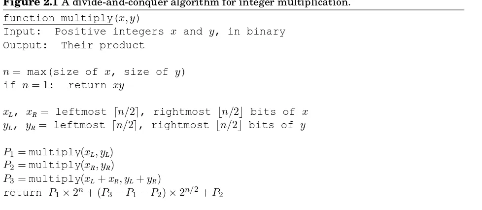
Figure 1.1Multiplication `a la Franc¸ais.
function multiply(x, y)
Input: Two n-bit integers x and y, where y≥0
Output: Their product
if y = 0: return 0 z=multiply(x,⌊y/2⌋) if y is even:
return 2z else:
return x+ 2z
The same algorithm can thus be repackaged in different ways. For variety we adopt a third formulation, the recursive algorithm of Figure 1.1, which directly implements the rule
x·y =
2(x· ⌊y/2⌋) ifyis even x+ 2(x· ⌊y/2⌋) ifyis odd.
Is this algorithm correct? The preceding recursive rule is transparently correct; so check-ing the correctness of the algorithm is merely a matter of verifycheck-ing that it mimics the rule and that it handles the base case (y= 0) properly.
How long does the algorithm take? It must terminate after n recursive calls, because at each callyis halved—that is, its number of bits is decreased by one. And each recursive call requires these operations: a division by2(right shift); a test for odd/even (looking up the last bit); a multiplication by2(left shift); and possibly one addition, a total ofO(n)bit operations. The total time taken is thusO(n2), just as before.
Can we do better? Intuitively, it seems that multiplication requires adding aboutn multi-ples of one of the inputs, and we know that each addition is linear, so it would appear thatn2 bit operations are inevitable. Astonishingly, in Chapter 2 we’ll see that wecando significantly better!
Division is next. To divide an integer xby another integery 6= 0means to find a quotient qand a remainderr, wherex=yq+randr < y. We show the recursive version of division in Figure 1.2; like multiplication, it takes quadratic time. The analysis of this algorithm is the subject of Exercise 1.8.
1.2
Modular arithmetic
pro-Figure 1.2Division.
function divide(x, y)
Input: Two n-bit integers x and y, where y≥1
Output: The quotient and remainder of x divided by y
if x= 0: return (q, r) = (0,0) (q, r) =divide(⌊x/2⌋, y)
q= 2·q, r= 2·r
if x is odd: r=r+ 1 if r ≥y: r =r−y, q =q+ 1 return (q, r)
Figure 1.3Addition modulo 8.
0 0 0
+
=
6
3
1
cessors, numbers are restricted to some size,32bits say, which is considered generous enough for most purposes.
For the applications we are working toward—primality testing and cryptography—it is necessary to deal with numbers that are significantly larger than32bits, but whose range is nonetheless limited.
Modular arithmeticis a system for dealing with restricted ranges of integers. We definex
moduloN to be the remainder whenxis divided byN; that is, ifx =qN +r with0≤r < N, thenxmoduloNis equal tor. This gives an enhanced notion of equivalence between numbers: xandyarecongruent moduloN if they differ by a multiple ofN, or in symbols,
x≡y (modN) ⇐⇒ N divides(x−y).
For instance, 253 ≡ 13 (mod 60) because 253 −13 is a multiple of 60; more familiarly, 253 minutes is 4 hours and 13 minutes. These numbers can also be negative, as in 59 ≡ −1 (mod 60): when it is59minutes past the hour, it is also1minute short of the next hour.
One way to think of modular arithmetic is that it limits numbers to a predefined range
{0,1, . . . , N −1}and wraps around whenever you try to leave this range—like the hand of a clock (Figure 1.3).
N −1. For example, there are three equivalence classes modulo3:
· · · −9 −6 −3 0 3 6 9 · · ·
· · · −8 −5 −2 1 4 7 10 · · ·
· · · −7 −4 −1 2 5 8 11 · · ·
Any member of an equivalence class is substitutable for any other; when viewed modulo 3, the numbers5and11are no different. Under such substitutions, addition and multiplication remain well-defined:
Substitution rule Ifx≡x′ (modN)andy≡y′ (mod N), then:
x+y≡x′+y′ (modN) and xy ≡x′y′ (modN).
(See Exercise 1.9.) For instance, suppose you watch an entire season of your favorite television show in one sitting, starting at midnight. There are25episodes, each lasting3hours. At what time of day are you done? Answer: the hour of completion is (25×3) mod 24, which (since 25≡1 mod 24) is1×3 = 3 mod 24, or three o’clock in the morning.
It is not hard to check that in modular arithmetic, the usual associative, commutative, and distributive properties of addition and multiplication continue to apply, for instance:
x+ (y+z)≡(x+y) +z (modN) Associativity
xy≡yx (modN) Commutativity
x(y+z)≡xy+yz (modN) Distributivity
Taken together with the substitution rule, this implies that while performing a sequence of arithmetic operations, it is legal to reduce intermediate results to their remainders modulo N at any stage. Such simplifications can be a dramatic help in big calculations. Witness, for instance:
2345≡(25)69≡3269≡169≡1 (mod 31).
1.2.1 Modular addition and multiplication
Toaddtwo numbersxandymoduloN, we start with regular addition. Sincexandyare each in the range0 to N −1, their sum is between 0and2(N −1). If the sum exceeds N −1, we merely need to subtract offN to bring it back into the required range. The overall computation therefore consists of an addition, and possibly a subtraction, of numbers that never exceed 2N. Its running time is linear in the sizes of these numbers, in other words O(n), where n=⌈logN⌉is the size ofN; as a reminder, our convention is to use the letternto denote input size.
To multiplytwo mod-N numbersx andy, we again just start with regular multiplication and then reduce the answer moduloN. The product can be as large as(N−1)2, but this is still
Two’s complement
Modular arithmetic is nicely illustrated intwo’s complement, the most common format for storing signed integers. It usesn bits to represent numbers in the range[−2n−1,2n−1 −1] and is usually described as follows:
• Positive integers, in the range 0 to 2n−1−1, are stored in regular binary and have a leading bit of0.
• Negative integers −x, with 1 ≤ x ≤ 2n−1, are stored by first constructingx in binary,
then flipping all the bits, and finally adding 1. The leading bit in this case is1.
(And the usual description of addition and multiplication in this format is even more arcane!) Here’s a much simpler way to think about it: any number in the range−2n−1 to2n−1−1 is stored modulo2n. Negative numbers−xtherefore end up as2n−x. Arithmetic operations like addition and subtraction can be performed directly in this format, ignoring any overflow bits that arise.
compute the remainder upon dividing it byN, using our quadratic-time division algorithm. Multiplication thus remains a quadratic operation.
Divisionis not quite so easy. In ordinary arithmetic there is just one tricky case—division by zero. It turns out that in modular arithmetic there are potentially other such cases as well, which we will characterize toward the end of this section. Whenever division is legal, however, it can be managed in cubic time,O(n3).
To complete the suite of modular arithmetic primitives we need for cryptography, we next turn tomodular exponentiation, and then to thegreatest common divisor, which is the key to division. For both tasks, the most obvious procedures take exponentially long, but with some ingenuity polynomial-time solutions can be found. A careful choice of algorithm makes all the difference.
1.2.2 Modular exponentiation
In the cryptosystem we are working toward, it is necessary to computexy modN for values of x,y, andN that are several hundred bits long. Can this be done quickly?
The result is some number moduloN and is therefore itself a few hundred bits long. How-ever, the raw value ofxy could be much, much longer than this. Even whenx andy are just 20-bit numbers,xy is at least(219)(219)= 2(19)(524288), about10million bits long! Imagine what happens ifyis a500-bit number!
To make sure the numbers we are dealing with never grow too large, we need to perform all intermediate computations moduloN. So here’s an idea: calculatexy modN by repeatedly multiplying byxmoduloN. The resulting sequence of intermediate products,
Figure 1.4Modular exponentiation.
function modexp(x, y, N)
Input: Two n-bit integers x and N, an integer exponent y
Output: xy modN
if y = 0: return 1 z=modexp(x,⌊y/2⌋, N) if y is even:
return z2 modN else:
return x·z2modN
consists of numbers that are smaller than N, and so the individual multiplications do not take too long. But there’s a problem: ify is 500 bits long, we need to perform y −1 ≈ 2500 multiplications! This algorithm is clearly exponential in the size ofy.
Luckily, wecando better: starting withxandsquaring repeatedlymoduloN, we get xmodN →x2 modN →x4 modN →x8 modN → · · · →x2⌊logy⌋ modN.
Each takes justO(log2N)time to compute, and in this case there are onlylogymultiplications. To determine xy modN, we simply multiply together an appropriate subset of these powers, those corresponding to1’s in the binary representation ofy. For instance,
x25 = x110012 = x100002 ·x10002 ·x12 = x16·x8·x1.
A polynomial-time algorithm is finally within reach!
We can package this idea in a particularly simple form: the recursive algorithm of Fig-ure 1.4, which works by executing, moduloN, the self-evident rule
xy =
(x⌊y/2⌋)2 ifyis even x·(x⌊y/2⌋)2 ifyis odd.
In doing so, it closely parallels our recursive multiplication algorithm (Figure 1.1). For in-stance, that algorithm would compute the productx·25by an analogous decomposition to the one we just saw: x·25 = x·16 +x·8 +x·1. And whereas for multiplication the terms x·2i come from repeated doubling, for exponentiation the corresponding terms x2i are generated by repeated squaring.
Letnbe the size in bits ofx,y, andN (whichever is largest of the three). As with multipli-cation, the algorithm will halt after at mostnrecursive calls, and during each call it multiplies n-bit numbers (doing computation moduloN saves us here), for a total running time ofO(n3).
1.2.3 Euclid’s algorithm for greatest common divisor
Figure 1.5Euclid’s algorithm for finding the greatest common divisor of two numbers.
function Euclid(a, b)
Input: Two integers a and b with a≥b≥0 Output: gcd(a, b)
if b= 0: return a return Euclid(b, amodb)
The most obvious approach is to first factor a and b, and then multiply together their common factors. For instance,1035 = 32·5·23and759 = 3·11·23, so their gcd is3·23 = 69.
However, we have no efficient algorithm for factoring. Is there some other way to compute greatest common divisors?
Euclid’s algorithm uses the following simple formula.
Euclid’s rule Ifxandyare positive integers withx≥y, thengcd(x, y) = gcd(xmody, y). Proof. It is enough to show the slightly simpler rulegcd(x, y) = gcd(x−y, y)from which the one stated can be derived by repeatedly subtractingyfromx.
Here it goes. Any integer that divides bothx andymust also dividex−y, sogcd(x, y) ≤ gcd(x−y, y). Likewise, any integer that divides bothx−yandy must also divide bothxand y, sogcd(x, y)≥gcd(x−y, y).
Euclid’s rule allows us to write down an elegant recursive algorithm (Figure 1.5), and its correctness follows immediately from the rule. In order to figure out its running time, we need to understand how quickly the arguments(a, b)decrease with each successive recursive call. In a single round, arguments(a, b)become(b, amodb): their order is swapped, and the larger of them,a, gets reduced toamodb. This is a substantial reduction.
Lemma Ifa≥b, thenamodb < a/2.
Proof. Witness that either b ≤ a/2or b > a/2. These two cases are shown in the following figure. Ifb≤a/2, then we haveamodb < b≤a/2; and ifb > a/2, thenamodb=a−b < a/2.
✁✁
✂✁✂✁✂ ✄✁✄✁✄✁✄☎✁☎✁☎✁☎
a a/2 b a
amodb b
amodb
a/2
Figure 1.6A simple extension of Euclid’s algorithm.
function extended-Euclid(a, b)
Input: Two positive integers a and b with a≥b≥0
Output: Integers x, y, d such that d= gcd(a, b) and ax+by=d
if b= 0: return (1,0, a)
(x′, y′, d) = Extended-Euclid(b, amodb) return (y′, x′− ⌊a/b⌋y′, d)
1.2.4 An extension of Euclid’s algorithm
A small extension to Euclid’s algorithm is the key to dividing in the modular world.
To motivate it, suppose someone claims that dis the greatest common divisor of aandb: how can we check this? It is not enough to verify thatddivides bothaandb, because this only showsdto be a common factor, not necessarily the largest one. Here’s a test that can be used ifdis of a particular form.
Lemma Ifddivides bothaandb, andd=ax+byfor some integersxandy, then necessarily d= gcd(a, b).
Proof. By the first two conditions,dis a common divisor ofaandband so it cannot exceed the greatest common divisor; that is,d≤gcd(a, b). On the other hand, sincegcd(a, b)is a common divisor ofaandb, it must also divideax+by = d, which impliesgcd(a, b) ≤d. Putting these together,d= gcd(a, b).
So, if we can supply two numbers x andy such that d = ax+by, then we can be sure d= gcd(a, b). For instance, we knowgcd(13,4) = 1because13·1 + 4·(−3) = 1. But when can we find these numbers: under what circumstances cangcd(a, b)be expressed in this checkable form? It turns out that italwayscan. What is even better, the coefficientsxandycan be found by a small extension to Euclid’s algorithm; see Figure 1.6.
Lemma For any positive integersaandb, the extended Euclid algorithm returns integersx, y, anddsuch thatgcd(a, b) =d=ax+by.
Proof. The first thing to confirm is that if you ignore thex’s andy’s, the extended algorithm is exactly the same as the original. So, at least we computed= gcd(a, b).
For the rest, the recursive nature of the algorithm suggests a proof by induction. The recursion ends whenb= 0, so it is convenient to do induction on the value ofb.
The base case b = 0 is easy enough to check directly. Now pick any larger value of b. The algorithm finds gcd(a, b) by calling gcd(b, amodb). Sinceamodb < b, we can apply the inductive hypothesis to this recursive call and conclude that thex′andy′it returns are correct:
Writing(amodb)as(a− ⌊a/b⌋b), we find
d= gcd(a, b) = gcd(b, amodb) = bx′+(amodb)y′ = bx′+(a−⌊a/b⌋b)y′ = ay′+b(x′−⌊a/b⌋y′).
Therefored=ax+bywithx=y′andy=x′−⌊a/b⌋y′, thus validating the algorithm’s behavior on input(a, b).
Example.To compute gcd(25,11), Euclid’s algorithm would proceed as follows: 25 = 2·11 + 3
11 = 3·3 + 2 3 = 1·2 + 1 2 = 2·1 + 0
(at each stage, the gcd computation has been reduced to the underlined numbers). Thus gcd(25,11) = gcd(11,3) = gcd(3,2) = gcd(2,1) = gcd(1,0) = 1.
To find x and y such that 25x+ 11y = 1, we start by expressing 1 in terms of the last pair(1,0). Then we work backwards and express it in terms of(2,1),(3,2),(11,3), and finally (25,11). The first step is:
1 = 1−0.
To rewrite this in terms of(2,1), we use the substitution0 = 2−2·1from the last line of the gcd calculation to get:
1 = 1−(2−2·1) =−1·2 + 3·1.
The second-last line of the gcd calculation tells us that1 = 3−1·2. Substituting: 1 =−1·2 + 3(3−1·2) = 3·3−4·2.
Continuing in this same way with substitutions2 = 11−3·3and3 = 25−2·11gives: 1 = 3·3−4(11−3·3) =−4·11 + 15·3 =−4·11 + 15(25−2·11) = 15·25−34·11.
We’re done:15·25−34·11 = 1, sox= 15andy=−34.
1.2.5 Modular division
In real arithmetic, every numbera6= 0 has an inverse,1/a, and dividing byais the same as multiplying by this inverse. In modular arithmetic, we can make a similar definition.
We sayxis themultiplicative inverseofamoduloN ifax≡1 (mod N).
There can be at most one such x modulo N (Exercise 1.23), and we shall denote it by a−1.
form ax+kN. So if gcd(a, N) > 1, then ax 6≡ 1 modN, no matter what x might be, and thereforeacannot have a multiplicative inverse moduloN.
In fact, this is the only circumstance in whichais not invertible. When gcd(a, N) = 1(we say a andN are relatively prime), the extended Euclid algorithm gives us integers x andy such thatax+N y= 1, which means thatax≡1 (mod N). Thusxisa’s sought inverse.
Example. Continuing with our previous example, suppose we wish to compute11−1 mod 25. Using the extended Euclid algorithm, we find that15·25−34·11 = 1. Reducing both sides modulo25, we have−34·11≡1 mod 25. So−34≡16 mod 25is the inverse of11 mod 25. Modular division theorem For any amodN, ahas a multiplicative inverse modulo N if and only if it is relatively prime toN. When this inverse exists, it can be found in timeO(n3)
(where as usualndenotes the number of bits ofN) by running the extended Euclid algorithm.
This resolves the issue of modular division: when working modulo N, we can divide by numbers relatively prime toN—and only by these. And to actually carry out the division, we multiply by the inverse.
Is your social security number a prime?
The numbers7,17,19,71,and79are primes, but how about 717-19-7179? Telling whether a reasonably large number is a prime seems tedious because there are far too many candidate factors to try. However, there are some clever tricks to speed up the process. For instance, you can omit even-valued candidates after you have eliminated the number 2. You can actually omit all candidates except those that are themselves primes.
In fact, a little further thought will convince you that you can proclaimN a prime as soon as you have rejected all candidatesup to √N, for ifN can indeed be factored as N =K·L, then it is impossible for both factors to exceed √N.
We seem to be making progress! Perhaps by omitting more and more candidate factors, a truly efficient primality test can be discovered.
Unfortunately, there is no fast primality test down this road. The reason is that we have been trying to tell if a number is a primeby factoring it. And factoring is a hard problem!
Modern cryptography, as well as the balance of this chapter, is about the following im-portant idea: factoring is hard and primality is easy. We cannot factor large numbers, but we can easily test huge numbers for primality! (Presumably, if a number is composite, such a test will detect thiswithout finding a factor.)
1.3
Primality testing
Fermat’s little theorem Ifpis prime, then for every1≤a < p, ap−1≡1 (modp).
Proof. LetS be the nonzero integers modulop; that is,S ={1,2, . . . , p−1}. Here’s the crucial observation: the effect of multiplying these numbers by a (modulo p) is simply to permute them. For instance, here’s a picture of the casea= 3, p= 7:
6 5 4 3 2
1 1
2
3
4
5
6
Let’s carry this example a bit further. From the picture, we can conclude
{1,2, . . . ,6} = {3·1 mod 7, 3·2 mod 7, . . . , 3·6 mod 7}.
Multiplying all the numbers in each representation then gives6!≡36·6! (mod 7), and dividing
by6!we get36 ≡1 (mod 7), exactly the result we wanted in the casea= 3, p= 7.
Now let’s generalize this argument to other values of a andp, with S = {1,2, . . . , p−1}. We’ll prove that when the elements ofS are multiplied byamodulop, the resulting numbers are all distinct and nonzero. And since they lie in the range[1, p−1], they must simply be a permutation ofS.
The numbersa·imodpare distinct because ifa·i≡a·j (modp), then dividing both sides byagives i≡j (modp). They are nonzero becausea·i≡0similarly impliesi≡0. (And we candivide bya, because by assumption it is nonzero and therefore relatively prime top.)
We now have two ways to write setS:
S = {1,2, . . . , p−1} = {a·1 modp, a·2 modp, . . . , a·(p−1) modp}.
We can multiply together its elements in each of these representations to get (p−1)!≡ap−1·(p−1)! (mod p).
Dividing by(p−1)! (which we can do because it is relatively prime top, since p is assumed prime) then gives the theorem.
Figure 1.7An algorithm for testing primality.
function primality(N)
Input: Positive integer N
Output: yes/no
Pick a positive integer a < N at random if aN−1 ≡1 (mod N):
return yes else:
return no
IsaN−1≡1 modN?
Pick somea
“prime”
“composite” Fermat’s test
Pass
Fail
The problem is that Fermat’s theorem is not an if-and-only-if condition; it doesn’t say what happens when N is not prime, so in these cases the preceding diagram is questionable. In fact, it is possible for a composite number N to pass Fermat’s test (that is, aN−1 ≡ 1 mod
N) for certain choices of a. For instance, 341 = 11·31 is not prime, and yet 2340 ≡ 1 mod 341. Nonetheless, we might hope that for composite N, most values of a will fail the test. This is indeed true, in a sense we will shortly make precise, and motivates the algorithm of Figure 1.7: rather than fixing an arbitrary value ofain advance, we should choose itrandomly from{1, . . . , N−1}.
In analyzing the behavior of this algorithm, we first need to get a minor bad case out of the way. It turns out that certain extremely rare composite numbersN, calledCarmichael num-bers, pass Fermat’s test forall arelatively prime to N. On such numbers our algorithm will fail; but they are pathologically rare, and we will later see how to deal with them (page 38), so let’s ignore these numbers for the time being.
In a Carmichael-free universe, our algorithm works well. Any prime number N will of course pass Fermat’s test and produce the right answer. On the other hand, any non-Carmichael composite numberN must fail Fermat’s test for some value of a; and as we will now show, this implies immediately that N fails Fermat’s test for at least half the possible values ofa!
Lemma IfaN−1 6≡ 1 modN for somearelatively prime to N, then it must hold for at least
half the choices ofa < N.
Proof. Fix some value ofafor whichaN−1 6≡1 modN. The key is to notice that every element b < N that passes Fermat’s test with respect toN (that is,bN−1 ≡1 modN) has a twin,a·b,
that fails the test:
Moreover, all these elements a·b, for fixed a but different choices of b, are distinct, for the same reasona·i6≡a·jin the proof of Fermat’s test: just divide bya.
Fail Pass
The set{1,2, . . . , N−1}
b a·b
The one-to-one functionb7→a·bshows that at least as many elements fail the test as pass it.
Hey, that was group theory!
For any integerN, the set of all numbers modN that are relatively prime to N constitute what mathematicians call agroup:
• There is a multiplication operation defined on this set.
• The set contains a neutral element (namely1: any number multiplied by this remains unchanged).
• All elements have a well-defined inverse.
This particular group is called themultiplicative group ofN, usually denotedZ∗
N.
Group theory is a very well developed branch of mathematics. One of its key concepts is that a group can contain a subgroup—a subset that is a group in and of itself. And an important fact about a subgroup is that its size must divide the size of the whole group.
Consider now the setB ={b:bN−1≡1 modN}. It is not hard to see that it is a subgroup
ofZ∗
N (just check that B is closed under multiplication and inverses). Thus the size of B must divide that ofZ∗
N. Which means that ifB doesn’t contain all of Z∗N, the next largest size it can have is|Z∗
N|/2.
We are ignoring Carmichael numbers, so we can now assert IfN is prime, thenaN−1≡1 modN for alla < N.
IfN is not prime, thenaN−1≡1 modN for at most half the values ofa < N.
The algorithm of Figure 1.7 therefore has the following probabilistic behavior. Pr(Algorithm 1.7 returnsyeswhenN is prime) = 1 Pr(Algorithm 1.7 returnsyeswhenN is not prime) ≤ 1
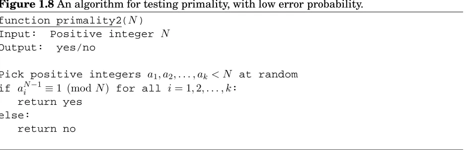
Figure 1.8An algorithm for testing primality, with low error probability.
function primality2(N)
Input: Positive integer N
Output: yes/no
Pick positive integers a1, a2, . . . , ak< N at random
if aNi −1 ≡1 (mod N) for all i= 1,2, . . . , k: return yes
else:
return no
We can reduce thisone-sided errorby repeating the procedure many times, by randomly pick-ing several values ofaand testing them all (Figure 1.8).
Pr(Algorithm 1.8 returnsyeswhenN is not prime) ≤ 1 2k
This probability of error drops exponentially fast, and can be driven arbitrarily low by choos-ingklarge enough. Testingk= 100values ofamakes the probability of failure at most2−100,
which is miniscule: far less, for instance, than the probability that a random cosmic ray will sabotage the computer during the computation!
1.3.1 Generating random primes
We are now close to having all the tools we need for cryptographic applications. The final piece of the puzzle is a fast algorithm for choosing random primes that are a few hundred bits long. What makes this task quite easy is that primes are abundant—a randomn-bit number has roughly a one-in-nchance of being prime (actually about1/(ln 2n)≈1.44/n). For instance, about 1 in 20 social security numbers is prime!
Lagrange’s prime number theorem Let π(x) be the number of primes≤x. Thenπ(x) ≈ x/(lnx), or more precisely,
lim x→∞
π(x) (x/lnx) = 1.
Such abundance makes it simple to generate a randomn-bit prime:
• Pick a randomn-bit numberN.
• Run a primality test onN.
Carmichael numbers
The smallest Carmichael number is561. It is not a prime: 561 = 3·11·17; yet it fools the Fermat test, becausea560≡1 (mod 561)for all values ofarelatively prime to561. For a long time it was thought that there might be only finitely many numbers of this type; now we know they are infinite, but exceedingly rare.
Thereisa way around Carmichael numbers, using a slightly more refined primality test due to Rabin and Miller. Write N −1 in the form 2tu. As before we’ll choose a random base aand check the value ofaN−1modN. Perform this computation by first determining au modN and then repeatedly squaring, to get the sequence:
aumodN, a2u modN, . . . , a2tu =aN−1 modN.
If aN−1 6≡1 modN, then N is composite by Fermat’s little theorem, and we’re done. But if
aN−1 ≡1 modN, we conduct a little follow-up test: somewhere in the preceding sequence, we ran into a1for the first time. If this happened after the first position (that is, ifaumodN 6= 1), and if the preceding value in the list is not−1 modN, then we declareN composite.
In the latter case, we have found anontrivial square root of 1 moduloN: a number that is not ±1 modN but that when squared is equal to1 modN. Such a number can only exist ifN is composite (Exercise 1.40). It turns out that if we combine this square-root check with our earlier Fermat test, then at least three-fourths of the possible values ofabetween1and N −1will reveal a compositeN, even if it is a Carmichael number.
How fast is this algorithm? If the randomly chosen N is truly prime, which happens with probability at least 1/n, then it will certainly pass the test. So on each iteration, this procedure has at least a1/nchance of halting. Therefore on average it will halt withinO(n) rounds (Exercise 1.34).
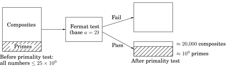
Next, exactly which primality test should be used? In this application, since the numbers we are testing for primality are chosen at random rather than by an adversary, it is sufficient to perform the Fermat test with base a = 2 (or to be really safe, a = 2,3,5), because for random numbers the Fermat test has a much smaller failure probability than the worst-case 1/2 bound that we proved earlier. Numbers that pass this test have been jokingly referred to as “industrial grade primes.” The resulting algorithm is quite fast, generating primes that are hundreds of bits long in a fraction of a second on a PC.
The important question that remains is: what is the probability that the output of the al-gorithm is really prime? To answer this we must first understand how discerning the Fermat test is. As a concrete example, suppose we perform the test with basea = 2for all numbers N ≤25×109. In this range, there are about109primes, and about20,000composites that pass
✁✁✁✁✁
all numbers≤25×109 After primality test
Primes
Randomized algorithms: a virtual chapter
Surprisingly—almost paradoxically—some of the fastest and most clever algorithms we have rely on chance: at specified steps they proceed according to the outcomes of random coin tosses. Theserandomized algorithmsare often very simple and elegant, and their output is correctwith high probability. This success probability does not depend on the randomness of the input; it only depends on the random choices made by the algorithm itself.
Instead of devoting a special chapter to this topic, in this book we intersperse randomized algorithms at the chapters and sections where they arise most naturally. Furthermore, no specialized knowledge of probability is necessary to follow what is happening. You just need to be familiar with the concept of probability, expected value, the expected number of times we must flip a coin before getting heads, and the property known as “linearity of expectation.”
Here are pointers to the major randomized algorithms in this book: One of the earliest and most dramatic examples of a randomized algorithm is the randomized primality test of Figure 1.8. Hashing is a general randomized data structure that supports inserts, deletes, and lookups and is described later in this chapter, in Section 1.5. Randomized algorithms for sorting and median finding are described in Chapter 2. A randomized algorithm for the min cut problem is described in the box on page 150. Randomization plays an important role in heuristics as well; these are described in Section 9.3. And finally the quantum algorithm for factoring (Section 10.7) works very much like a randomized algorithm, its output being correct with high probability—except that it draws its randomness not from coin tosses, but from the superposition principle in quantum mechanics.
Virtual exercises: 1.29, 1.34, 2.24, 9.8, 10.8.
1.4
Cryptography
The typical setting for cryptography can be described via a cast of three characters: Alice and Bob, who wish to communicate in private, and Eve, an eavesdropper who will go to great lengths to find out what they are saying. For concreteness, let’s say Alice wants to send a specific message x, written in binary (why not), to her friend Bob. She encodes it as e(x), sends it over, and then Bob applies his decryption functiond(·)to decode it:d(e(x)) =x. Here e(·)andd(·)are appropriate transformations of the messages.
Eve
Bob Alice
Encoder Decoder
x e(x) x=d(e(x))
Alice and Bob are worried that the eavesdropper, Eve, will intercepte(x): for instance, she might be a sniffer on the network. But ideally the encryption functione(·) is so chosen that without knowing d(·), Eve cannot do anything with the information she has picked up. In other words, knowinge(x)tells her little or nothing about whatxmight be.
For centuries, cryptography was based on what we now callprivate-key protocols. In such a scheme, Alice and Bob meet beforehand and together choose a secret codebook, with which they encrypt all future correspondence between them. Eve’s only hope, then, is to collect some encoded messages and use them to at least partially figure out the codebook.
An application of number theory?
The renowned mathematician G. H. Hardy once declared of his work: “I have never done anything useful.” Hardy was an expert in the theory of numbers, which has long been re-garded as one of the purest areas of mathematics, untarnished by material motivation and consequence. Yet the work of thousands of number theorists over the centuries, Hardy’s in-cluded, is now crucial to the operation of Web browsers and cell phones and to the security of financial transactions worldwide.
1.4.1 Private-key schemes: one-time pad and AES
If Alice wants to transmit an important private message to Bob, it would be wise of her to scramble it with an encryption function,
e:hmessagesi → hencoded messagesi.
Of course, this function must be invertible—for decoding to be possible—and is therefore a bijection. Its inverse is the decryption functiond(·).
In the one-time pad, Alice and Bob meet beforehand and secretly choose a binary string r of the same length—say, n bits—as the important message x that Alice will later send. Alice’s encryption function is then a bitwise exclusive-or, er(x) = x⊕r: each position in the encoded message is the exclusive-or of the corresponding positions inxandr. For instance, if r= 01110010, then the message11110000is scrambled thus:
er(11110000) = 11110000⊕01110010 = 10000010.
This functioner is a bijection fromn-bit strings ton-bit strings, as evidenced by the fact that it is its own inverse!
er(er(x)) = (x⊕r)⊕r = x⊕(r⊕r) = x⊕0 = x,
where 0is the string of all zeros. Thus Bob can decode Alice’s transmission by applying the same encryption function a second time: dr(y) =y⊕r.
How should Alice and Bob chooserfor this scheme to be secure? Simple: they should pick rat random, flipping a coin for each bit, so that the resulting string is equally likely to be any element of{0,1}n. This will ensure that if Eve intercepts the encoded messagey=e
r(x), she gets no information about x. Suppose, for example, that Eve finds outy = 10; what can she deduce? She doesn’t know r, and the possible values it can take all correspond to different original messagesx:
00
01
10
11
x
10
e11
e01 e00