A CAUCHY PROBLEM FOR HELMHOLTZ EQUATION: REGULARIZATION AND ERROR ESTIMATES
Nguyen Huy Tuan and Pham Hoang Quan
Abstract. In this paper, the Cauchy problem for the Helmholtz equation is investigated. It is known that such problem is severely ill-posed. We propose a new regularization method to solve it based on the solution given by the method of separation of variables. Error estimation and convergence analysis have been given. Finally, we present numerical results for several examples and show the effectiveness of the proposed method.
2000Mathematics Subject Classification: 35K05, 35K99, 47J06, 47H10. 1. Introduction
The Helmholtz equation arises in many physical applications (see, e.g., [1, 2, 4, 9, 12] and the references therein). The direct problem for Helmholtz equation, i.e., Dirich-let, Neumann or mixed boundary value problems have been studied extensively in the past century. However, in some practical problems, the boundary data on the whole boundary cannot be obtained. We only know the noisy data on a part of the boundary of the concerning domain, which will lead to some inverse prob-lems. The Cauchy problem for the Helmholtz equation is an inverse problem and is severely ill-posed [3]. That means the solution does not depend continuously on the given Cauchy data and any small perturbation in the given data may cause large change to the solution. In recent years, the Cauchy problems associated with the Helmholtz equation have been studied by using different numerical methods, such as the Landweber method with boundary element method (BEM) [8], the conju-gate gradient method [7], the method of fundamental solutions (MFS) [14] and so on. However, most of numerical methods are short of stability analysis and error estimate.
solving a Cauchy problem of modified Helmhotlz equation where they consider a homogenous Neumann boundary condition, the results are less encouraging. The main aim of this paper is to present a new regularization method, and investigate the error estimate between the regularization solution and the exact one.
The paper is organized as follows. In Section 2, the regularization method is intro-duced; in Section 3, some stability estimates are proved under some priori conditions; in Section 4, some numerical results are reported.
2. Mathematical Problem And Regularization.
We consider the following Cauchy problem for the Helmholtz equation with nonho-mogeneous Neumman boundary condition
∆u+k2u= 0,(x, y)∈(0, π)×(0,1)
u(0, y) =u(π, y) = 0, y∈(0,1)
uy(x,0) =f(x),(x, y)∈(0, π)×(0,1)
u(x,0) =g(x),0< x < π
(1)
where g(x), f(x) is a given vector in L2(0, π) and 0< k <1 is the wave number. By the method of separation of variables, the solution of problem (1) is as follows
u(x, y) = ∞
X
n=1
"
e√n2−k2y+e−√n2−k2y 2
!
gn+
e√n2−k2y−e−√n2−k2y 2√n2−k2
!
fn #
sinnx (2)
where
f(x) = ∞
X
n=1
fnsinnx, g(x) =
∞
X
n=1
gnsinnx.
Physically,gcan only be measured, there will be measurement errors, and we would actually have as data some function gǫ ∈L2(0, π), for which
kgǫ−gk ≤ǫ
where the constant ǫ >0 represents a bound on the measurement error,k.kdenotes the L2-norm. Denote β is the regularization parameter depend onǫ.
The case f = 0, the problem (1) becomes
∆u+k2u= 0,(x, y)∈(0, π)×(0,1)
u(0, y) =u(π, y) = 0, y∈(0,1)
uy(x,0) = 0,(x, y)∈(0, π)×(0,1)
u(x,0) =g(x),0< x < π
Very recently, in [6], H.H.Quin and T.Wei considered (2) by the quasi-reversibility method. They established the following problem for a fourth-order equation
Separation of variables leads to the solution of problem (4) as follows
uǫ(x, y) = become large, so it is the unstability cause. To regularization the problem (2), we should replace it by the better terms. In (4), the authors replaced e√n2−k2y and
1+βn2y respectively. Notice the reader
that in the case k= 0, the problem (4) is also considered in [10](See page 481). To the author’s knowledge, although the problem (4) is investigated by some recent paper but there are rarely results of regularize method for treating the problem (3) until now. In this paper, we shall replace e√n2
−k2y by the different better terms
e(√n2−k2−β(n2−k2))y and modify the exact solutionu as follows
sponding to the noisy data gǫ
vǫ(x, y) =
3. Main Results
Theorem 1Letvǫandwǫbe the solution of problem (7)andvǫ(x,0) =gǫ(x), wǫ(x,0) =
hǫ(x). Assume that kgǫ−hǫk ≤ǫ, then we have
kvǫ(., y)−wǫ(., y)k ≤e41βǫ. (8)
Proof.
vǫ(x, y) = ∞
X
n=1
"
eA(β,n,k)y+e−√n2−k2y 2
!
gnǫ + e
A(β,n,k)y−e−√n2−k2y 2√n2−k2
!
fn #
sinnx. (9) and
wǫ(x, y) = ∞
X
n=1
"
eA(β,n,k)y+e−√n2−k2y 2
!
hǫn+ e
A(β,n,k)y−e−√n2−k2y 2√n2−k2
!
fn #
sinnx.(10)
where
hǫn= 2
π
Z π
0
hǫ(x) sin(nx)dx.
It follows from (9) and (10) that
vǫ(x, y)−wǫ(x, y) = ∞
X
n=1
eA(β,n,k)y+e−√n2−k2y 2
!
(gnǫ −hǫn) sinnx.
Using the inequality A(β, n, k)≤ 41β and (a+b)2 ≤2a2+ 2b2, we have
kvǫ(., y)−wǫ(., y)k2 = π 2
∞
X
n=1
eA(β,n,k)y+e−√n2−k2y 2
!2
|gnǫ −hǫn|2
≤ π 4(e
1 2ǫ + 1)
∞
X
n=1
|gnǫ −hǫn|2
≤ 12(e21β + 1)kg−hk2
≤ e21βǫ2. (11)
This completes the proof of Theorem 1.
Theorem 2.Let ku(.,1)k ≤A1. Let f be a function such that ∞
X
n=1
(n2−k2)2e2√n2−k2af2
Let β= ln1ǫ−1
then one has
ku(x, y)−vǫ(x, y)k ≤√ǫ+
This error order is the same in the Theorem 3.1, in [6].
Proof. We have
u(x, y)−uǫ(x, y) =
We also have
< u(x,1),sinnx >= e
It implies that
For k, n >0, it is easy to prove that (n2−k2)2
e2k√n2−k2) ≤
4
k4. Thus, for y <1
e2(y−1)√n2−k2)β2(n2−k2)2 ≤ 4β 2 (1−y)4. This follows that
|< u(x, y)−uǫ(x, y),sinnx >|2 ≤ 4β
2
(1−y)4 < u(x,1),sinnx >| 2+1
2β 2(n2
−k2)2e2√n2−k2)yf2
n.
Thus
ku(x, y)−uǫ(x, y)k2 = π 2
∞
X
n=1
|< u(x, y)−uǫ(x, y),sinnx >|2
≤ 2πβ 2 (1−y)4
∞
X
n=1
< u(x,1),sinnx >|2+π 4β
2X∞ n=1
(n2−k2)2e2√n2−k2)yf2
n
≤ 2β 2
(1−y)4ku(.,1)k 2+ π
4β 2A
2. (16)
From Theorem 1, we get
kvǫ(., y)−uǫ(., y)k ≤e41βǫ. (17)
Fromβ = ln1ǫ−1
and combining (11), (16) and (17), we obtain
ku(x, y)−vǫ(x, y)k ≤ ku(x, y)−uǫ(x, y)k+kuǫ(x, y)−vǫ(x, y)k ≤ e21βǫ+β
s
2
(1−y)4A1+
π
4A2 ≤ ǫ34 +
ln1
ǫ
−1s
2
(1−y)4A1+
π
4A2.
Theorem 3.Let f be as Theorem 2. Suppose thatu(.,1)satisfy the condition
∞
X
n=1
(n2−k2)2|< u(x,1),sinnx >|2< A3.
Let β= ln1ǫ−1
then one has
ku(x, y)−vǫ(x, y)k ≤
ln1
ǫ
−1r
π
2A3+
π
for every y∈[0,1], where vǫ is the unique solution of Problem (7) . Proof.It follows from (15) that
|< u(x, y)−uǫ(x, y),sinnx >|2 ≤ β2(n2−k2)2y2|< u(x,1),sinnx >|2+ +1
2β 2y2(n2
−k2)e2√n2−k2yf2
n.
Then
ku(x, y)−uǫ(x, y)k2 = π 2
∞
X
n=1
|< u(x, y)−uǫ(x, y),sinnx >|2
≤ π2β2(n2−k2)2y2|< u(x,1),sinnx >|2
+π 4β
2y2(n2−k2)e2√n2−k2y
fn2
≤ π2β2A3+
π
4β 2A
2. Therefore we get
ku(x, y)−uǫ(x, y)k ≤β
r
π
2A3+
π
4A2. (18)
Fromβ = ln1ǫ−1
and combining (11), (18), we obtain
ku(x, y)−vǫ(x, y)k ≤ ku(x, y)−uǫ(x, y)k+kuǫ(x, y)−vǫ(x, y)k ≤ β
r
π
2A3+
π
4A2+e 1 4βǫ
≤
ln1
ǫ
−1r
π
2A3+
π
4A2+ǫ 3 4.
4. Numerical Results
In this section, a simple example is devised for verifying the validity of the proposed method. For the reader can make a comparison between this paper with [6] by using same example with same parameters, we consider the problem
uxx+uyy+
1
4u= 0,(x, y)∈(0, π)×(0,1)
u(0, y) =u(π, y) = 0, y ∈(0,1)
uy(x,0) = 0,(x, y)∈(0, π)×(0,1)
u(x,0) = sin(x),0< x < π
The exact solution to this problem is
Let gm be the measured data
gm(x) = sin(x) +
The solution of (19), corresponding thegm, is
um(x, t) = e Then, we notice that
lim
From the two equalities above, we see that (19) is an ill-posed problem. Hence, the Cauchy problem (19) cannot be solved by using classical numerical methods and it needs regularization techniques.
Letǫ=pπ
2m1. By approximating the problem as in (15), the regularized solution is
Table 1: The error of the method in this paper. +6.716243945×10−1100129330sin(1010x)
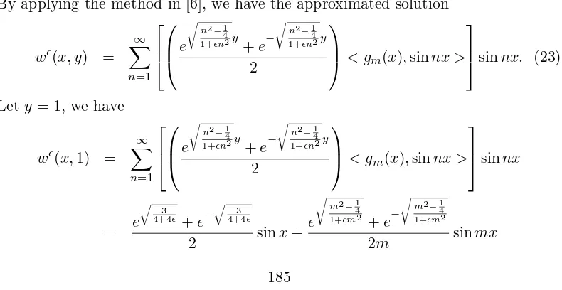
Let y= 1, the solution is written as
vǫ(x,1) = e
Table 1 shows the the error between the regularization solution vǫ and the exact solution u, for three values of ǫ. We have the table numerical test by choose some values as follows
1. ǫ= 10−2pπ
By applying the method in [6], we have the approximated solution
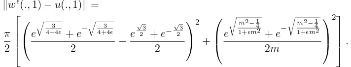
kwǫ(.,1)−u(.,1)k=
π
2
e q
3 4+4ǫ +e−
q
3 4+4ǫ
2 −
e √
3 2 +e−
√
3 2 2
2 +
e r
m2−1 4 1+ǫm2 +e−
r
m2−1 4 1+ǫm2
2m
2
.
We note that if we choose ǫandmsuch thatǫ=pπ
2m1 thenkwǫ(.,1)−u(.,1)kdoes
not converges to zero. Thus, to compare the error of two method, we choose some same parameter values to get the table numerical test as follows
1. ǫ= 10−2pπ
2 corresponding to m= 104. 2. ǫ= 10−3pπ
2 corresponding to m= 1015. 3. ǫ= 10−4pπ
2 corresponding to m= 1020.
Table 2: The error of the method in the paper [6]
ǫ wǫ kwǫ−uk
10−2pπ
2 v1= 1.39379109494861 sin(x) + 0.3786841911 sin(104x) 0.474655690138409 10−3pπ
2 1.39850107010763 sin(x) + 0.0009255956190 sin(1015x) 0.00133695472487849 10−4pπ
2 1.39850107010763 sin(x) + 9.255956190×10⁻¹⁰sin(1020x) 0.000664608094405560
Looking at Tables 1,2,3 a comparison between the two methods, we can see the error results of in Table 3 are smaller than the errors in Tables 2. In the same parameter regularization, the error is Table 1 and 3 converges to zero more quickly many times than the Table 2 . This shows that our approach has a nice regularizing effect and give a better approximation with comparison to the many previous results, such as [5, 6, 14].
Table 3: The different error of the method in this paper.
ǫ vǫ aǫ =kvǫ(.,1)−u(.,1)k
ǫ1= 10−2pπ2 1.38790989314992 sin(x) 0.0139386799063127 +5,667504490×10−4348sin(104×x)
ǫ2= 10−3pπ2 1.39891961780226 sin(x) 0.000140036351583956 +7.548683905×10−4342953sin(1015x)
References
[1] T. DeLillo, V. Isakov, N. Valdivia, L. Wang, The detection of the source of acoustical noise in two dimensions, SIAM J. Appl. Math. 61 (2001) 21042121. [2] T. DeLillo, V. Isakov, N. Valdivia, L. Wang,The detection of surface vibrations
from interior acoustical pressure, Inverse Problems 19 (2003) 507524.
[3] J. Hadamard,Lectures on Cauchys Problem in Linear Partial Differential Equa-tions, Dover Publications, New York, 1953.
[4] W.S. Hall, X.Q. Mao, Boundary element investigation of irregular frequencies in electromagnetic scattering, Eng. Anal. Bound. Elem. 16 (1995) 245252. [5] D. N. Hao and D. Lesnic ,The Cauchy for Laplaces equation via the conjugate
gradient method, IMA Journal of Applied Mathematics, 65:199-217(2000). [6] Hai-Hua Qin, Ting Wei,Modified regularization method for the Cauchy problem
of the Helmholtz equation, Appl. Math. Model. 33 (2009), no. 5, 2334–2348. [7] L. Marin, L. Elliott, P.J. Heggs, D.B. Ingham, D. Lesnic, X. Wen, Conjugate
gradient-boundary element solution to the Cauchy problem for Helmholtz-type equations, Comput. Mech. 31 (34) (2003) 367377.
[8] L. Marin, L. Elliott, P. Heggs, D. Ingham, D. Lesnic, X.Wen,BEM solution for the Cauchy problem associated with Helmholtz-type equations by the Landweber method, Eng. Anal. Boundary Elem. 28 (9) (2004) 10251034.
[9] L. Marin, L. Elliott, P.J. Heggs, D.B. Ingham, D. Lesnic, X. Wen,An alternating iterative algorithm for the Cauchy problem associated the Helmholtz equation, Comput. Methods Appl. Mech. Engrg. 192 (2003) 709722.
[10] Z. Qian, C.L. Fu, Z.P. Li,Two regularization methods for a Cauchy problem for the Laplace equation, J. Math. Anal. Appl. 338 (1) (2008) 479489.
[11] Z. Qian, C.-L. Fu, X.-T. Xiong, Fourth-order modified method for the Cauchy problem for the Laplace equation, J. Comput. Appl. Math. 192 (2) (2006) 205218.
[12] T. Reginska, K. Reginski, Approximate solution of a Cauchy problem for the Helmholtz equation, Inverse Problems 22 (2006) 975989.
[14] T.Wei, Y. Hon, L. Ling, Method of fundamental solutions with regularization techniques for Cauchy problems of elliptic operators, Eng. Anal. Boundary Elem. 31 (4) (2007) 373385.
[15] A. Yoneta, M. Tsuchimoto, T. Honma, Analysis of axisymmetric modified Helmholtz equation by using boundary element method, IEEE Trans. Magn. 26 (2) (1990) 10151018.
Nguyen Huy Tuan
Department of Mathematics and Application SaiGon University
273 An Duong vuong street, HoChiMinh city, VietNam email:tuanhuy [email protected]
Pham Hoang Quan
Department of Mathematics and Application SaiGon University