ELECTRONIC
COMMUNICATIONS in PROBABILITY
INTERSECTION PROBABILITIES FOR A CHORDAL
SLE PATH AND A SEMICIRCLE
TOM ALBERTS
Courant Institute of Mathematical Sciences, 251 Mercer St. New York University, New York, NY 10012 USA
email: [email protected]
MICHAEL J. KOZDRON1
Department of Mathematics & Statistics, College West 307.14 University of Regina, Regina, SK S4S 0A2 Canada
email: [email protected]
Submitted March 7, 2008, accepted in final form July 22, 2008 AMS 2000 Subject classification: 82B21, 60K35, 60G99, 60J65
Keywords: Schramm-Loewner evolution, restriction property, Hausdorff dimension, swallowing time, intersection probability, Schwarz-Christoffel transformation.
Abstract
We derive a number of estimates for the probability that a chordal SLEκ path in the upper
half plane Hintersects a semicircle centred on the real line. We prove that if 0< κ <8 and
γ: [0,∞)→His a chordal SLEκ inHfrom 0 to ∞, thenP{γ[0,∞)∩ C(x;rx)6=∅} ≍r4a−1 wherea= 2/κandC(x;rx) denotes the semicircle centred atx >0 of radiusrx, 0< r≤1/3, in the upper half plane. As an application of our results, for 0< κ <8, we derive an estimate for the diameter of a chordal SLEκpath inHbetween two real boundary points 0 andx >0.
For 4 < κ < 8, we also estimate the probability that an entire semicircle on the real line is swallowed at once by a chordal SLEκpath in Hfrom 0 to∞.
1
Introduction
The Schramm-Loewner evolution (SLE) is a one-parameter family of random growth processes introduced by O. Schramm [9] which has been successfully used to establish a number of rigorous mathematical results about various two-dimensional models from statistical mechanics including percolation, loop-erased random walk, and the Ising model. There are actually two variants of SLE that one can consider. Radial SLE describes the growth of a curve connecting a given boundary point to a given interior point whereas chordal SLE describes the growth of a curve connecting two distinct boundary points. It is assumed that the reader is familiar with the basic properties of SLE as found in [7].
1SUPPORTED IN PART BY THE NATURAL SCIENCES AND ENGINEERING RESEARCH COUNCIL (NSERC) OF CANADA.
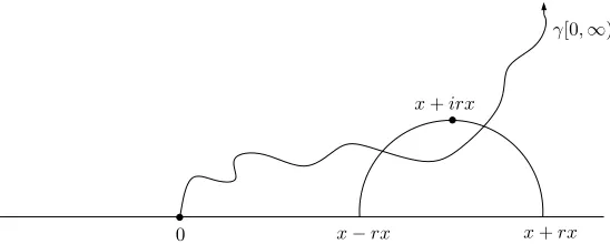
The primary purpose of this paper is to derive estimates for the probability that a chordal SLE path inHfrom 0 to∞intersects a semicircle in the upper half plane centred at a fixed point x > 0 on the real line. Specifically, suppose that γ : [0,∞) → H is (the trace of) a chordal SLEκ inHfrom 0 to∞where κ∈(0,8). For ǫ >0 andx∈R, denote the semicircle
of radiusǫ centred atx in the upper half plane byC(x;ǫ). In the 0< κ <8 regime, we will derive estimates for the intersection probability
P{γ[0,∞)∩ C(x;rx)6=∅}
where 0< r≤1/3 andx >0. An example is shown in Figure 1.
C(x;rx)
0 x−rx x+rx
γ[0,∞)
Figure 1: The event{γ[0,∞)∩ C(x;rx) =∅}in the 0< κ≤4 case.
We conclude the introduction with the statement of our primary theorems. Most of this paper is devoted to their proof. In the final section we give some applications of our results. Recall that
g(r)≍h(r) if there exist non-zero, finite constantsc1andc2such thatc1h(r)≤g(r)≤c2h(r). Furthermore,g(r)∼h(r) ifg(r)/h(r)→1 asr↓0.
Theorem 1.1. Supposex >0 is a real number,0< r≤1/3, andC(x;rx) ={x+rxeiθ: 0<
θ < π} denotes the semicircle of radiusrx centred atxin the upper half plane. If 0< κ <8 andγ: [0,∞)→His a chordal SLEκ in Hfrom0 to∞, then
P{γ[0,∞)∩ C(x;rx)6=∅} ≍r8−κκ.
By an appropriate conformal transformation, an equivalent formulation of Theorem 1.1 gives an estimate for the diameter of a chordal SLEκpath inHfrom 0 tox >0. This is illustrated
in Figure 2.
0 x Rx
C(0;Rx)
γ′[0, t γ]
Figure 2: The event{γ′[0, t
Corollary 1.2. Supposex >0 is a real number, R≥3, and C(0;Rx) ={Rxeiθ: 0< θ < π}
denotes the circle of radius Rx centred at 0 in the upper half plane. If 0 < κ < 8 and
γ′: [0, t
γ′]→His a chordal SLEκ in Hfrom0 tox, then
P{γ′[0, tγ′]∩ C(0;Rx)6=∅} ≍R
κ−8
κ .
Remark. In the particular case when κ = 8/3 it is possible to compute the intersection probabilities in Theorem 1.1 and Corollary 1.2 exactly. We show in Section 5 that if 0< r <1, then
P{γ[0,∞)∩ C(x;rx)=6 ∅}= 1−(1−r2)5/8, (1) and ifR >1, then
P{γ′[0, tγ′]∩ C(0;Rx)=6 ∅}= 1−(1−R−2)5/8.
As well, (1) implies
P{γ[0,∞)∩ C(x;rx)6=∅} ∼5
8r
2
as r↓0 which is consistent with Theorem 1.1.
The outline of the remainder of the paper is as follows. In Section 2, we introduce some nota-tion. The proof of Theorem 1.1 is then given in Section 3. In Section 4 we derive Corollary 1.2 and then conclude in Section 6 by using Theorem 1.1 to derive two other intersection proba-bilities for a chordal SLE path and a semicircle centred on the real line. (These are given by Theorem 6.1 and Corollary 6.2.) In particular, for 4< κ <8, we estimate the probability that an entire semicircle on the real line is swallowed at once by a chordal SLEκpath in Hfrom 0
to ∞.
2
Notation
We now introduce the notation that will be used throughout the remainder of the paper. Let Cdenote the set of complex numbers and writeH={z∈C:ℑ(z)>0} to denote the upper half plane. Ifǫ >0 andz∈C, we writeB(z;ǫ) ={w∈C:|z−w|< ǫ}for the ball of radiusǫ centred at z. Ifx∈R, then the half disk and semicircle of radiusǫcentred atxin the upper half plane are given by
D(x;ǫ) =B(x;ǫ)∩H={x+ρeiθ: 0< θ < π,0< ρ < ǫ} (2)
and
C(x;ǫ) =∂B(x;ǫ)∩H={x+ǫeiθ: 0< θ < π}, (3)
respectively.
The chordal Schramm-Loewner evolution in H from 0 to ∞ with parameter κ= 2/a is the solution of the differential equation
∂tgt(z) =
a gt(z)−Ut
, g0(z) =z, (4)
the chordal Loewner equation (4), and define the hullKtbyKt={z∈H:Tz< t}. The hulls
{Kt, t≥0}are an increasing family of compact sets inHandgtis a conformal transformation
ofH\KtontoH. For allκ >0, there is a continuous curve{γ(t), t≥0}withγ: [0,∞)→H andγ(0) = 0 such thatH\Ktis the unbounded connected component ofH\γ(0, t] a.s. The behaviour of the curve γ depends on the parameter κ (or, equivalently, the value of a). If
a ≥ 1/2 (i.e., 0 < κ ≤ 4), thenγ is a simple curve with γ(0,∞) ⊂H and Kt = γ(0, t]. If 1/4< a <1/2 (i.e., 4< κ <8), thenγ is a non-self-crossing curve with self-intersections and
γ(0,∞)∩R6=∅. Although the present work will not be concerned with the casea≤1/4 (i.e.,
κ≥8), it is worth recalling that for this regimeγis a space-filling, non-self-crossing curve. Let
µ#H(0,∞) denote the chordal SLEκprobability measure on paths inHfrom 0 to∞. IfD⊂C
is a simply connected domain and z, ware distinct points in∂D, thenµ#D(z, w), the chordal
SLEκ probability measure on paths in D from z to w, is defined to the image of µ#H(0,∞)
under a conformal transformationf :H→D withf(0) =z and f(∞) =w. In other words, SLEκin Dfromzto wis simply the conformal image of SLEκin Hfrom 0 to∞. For further
details about SLE, consult [7].
3
Proof of Theorem 1.1
In this section we prove Theorem 1.1. The proof is divided into three subsections. For the lower bound in both the 0< κ≤4 and 4< κ <8 cases, we are able to give an explicit value for the constant. For the upper bound, however, all that can be determined is the existence of a constant.
3.1
The upper bound
Throughout this section, suppose that γ : [0,∞) → His a chordal SLEκ in Hfrom 0 to ∞ with 0 < κ < 8 and a = 2/κ. The primary tool we need to establish the upper bound in Theorem 1.1 is originally due to Beffara [3, Proposition 2]. We briefly recall the statement here and refer the reader to [3] for further details.
Proposition 3.1. If z∈H,0< ǫ≤ ℑ{z}/2, andB(z;ǫ) ={w∈C:|z−w|< ǫ} denotes the ball of radiusǫcentred atz, then
P{γ[0,∞)∩ B(z;ǫ)6=∅} ≍
µ ǫ
ℑ{z}
¶1−41aµℑ{z} |z|
¶4a−1
where the constants implied by≍may depend ona.
We would like to stress that this proposition holds for alla >1/4 (equivalently, all 0< κ <8). The following theorem gives a careful statement of the upper bound that we will establish.
Theorem 3.2. Let 0< r≤1/3 andx >0. Ifγ: [0,∞)→His a chordal SLEκ inHfrom0 to∞with 0< κ <8anda= 2/κ, then there exists a constantca such that
P{γ[0,∞)∩ C(x;rx)6=∅} ≤car4a−1.
Figure 3: The semicircleC(x;rx) covered by a sequence of balls centred at{z±n, n= 0,1, . . .}.
Proof of Theorem 3.2. Setz0 =x+irx and forn= 1,2, . . ., let z±n =x±rx+irx2−|n|+1.
Using Proposition 3.1, it follows that
P as is clear from Figure 3. Hence, (5) implies that there exists a constant ca such that
P{γ[0,∞)∩ C(x;rx)6=∅} ≤
In this section we establish the lower bound in Theorem 1.1 for κ∈(4,8).
Theorem 3.3. Let0< r≤1/3 andx >0. If γ: [0,∞)→His a chordal SLEκ inHfrom 0 to∞ with4< κ <8 anda= 2/κ, then there exists a constant ca such that
0 x−rx x+rx
C(x, rx)
Figure 4: The event thatγ[0,∞) intersects the interval [x−rx, x+rx].
Proof. It is clear that ifγ[0,∞) intersects the interval [x−rx, x+rx] then it also intersects the semicircleC(x;rx), as Figure 4 shows. By Proposition 6.34 of [7] and the scale invariance of SLE,
P{γ[0,∞)∩[x−rx, x+rx]6=∅}= Γ(2a) Γ(1−2a)Γ(4a−1)
Z 1+2rr
0
dt t2−4a(1−t)2a
≥ Γ(2a)
Γ(1−2a)Γ(4a−1)
Z 1+2rr
0
dt t2−4a(1/2)2a
≥ Γ(2a)2 2a
Γ(1−4a)Γ(4a)(2r)
4a−1.
The first and second inequalities use 0< r ≤1/3. (Actually, all that is required here is that
r >0 be bounded away from 1. We took 0< r≤1/3 simply for convenience.)
3.3
The lower bound for
0
< κ
≤
4
In this section we establish the lower bound in Theorem 1.1 forκ∈(0,4).
Theorem 3.4. Let 0< r <1 andx >0. Ifγ: [0,∞)→His a chordal SLEκ inHfrom0 to
∞with 0< κ≤4anda= 2/κ, then there exists a constantca such that
P{γ[0,∞)∩ C(x;rx)6=∅} ≥car4a−1.
To prove the theorem we recall the probability that a fixed point z ∈ H lies to the left of
γ[0,∞). This result is originally due to Schramm [10], although the form that we include is from Garban and Trujillo Ferreras [5].
Proposition 3.5. Letz=ρeiθ ∈H, and setf(z) =P{z is to the left of γ[0,∞)}. By scaling,
the function f only depends onθ and is given by
f(θ) =
Rθ 0(sinα)
4a−2dα Rπ
0(sinα)4a−2dα .
Proof of Theorem 3.4. Figure 5 clearly shows that
P{γ[0,∞)∩ C(x;rx)=6 ∅} ≥P{x+irxis to the left ofγ[0,∞)}.
x−rx x+rx
x+irx
0
γ[0,∞)
Figure 5: The pointz=x+irxis to the left ofγ[0,∞).
Proposition 3.5 that
P{x+irxis to the left ofγ[0,∞)} · Z π
0
(sinα)4a−2dα=
Z arctan(r) 0
(sinα)4a−2dα
≥1
2
Z arctan(r)
0
α4a−2dα
=arctan
4a−1(r)
8a−2 . (6)
Since 8 arctant ≥πt for 0 ≤t ≤ 1, we see that (6) implies that there exists a constant ca,
namely
ca = π
4a−1
46a−1(4a−1)Rπ
0(sinα)4a−2dα ,
such thatP{x+irxis to the left ofγ[0,∞)} ≥car4a−1.
4
Estimating the diameter of a chordal SLE path
In this section, we derive Corollary 1.2 from Theorem 1.1. The proof is not difficult; the basic idea is to determine the appropriate conformal transformation and use the conformal invariance of chordal SLE. Recall that if D ⊂C is a simply connected domain and z, w are two distinct points in∂D, then chordal SLEκ inDfromz towis defined to be the conformal
image of chordal SLEκ in H from 0 to∞ as discussed in Section 2. Letx >0 be real, and
suppose that γ′ : [0, t
γ′] → H is an SLEκ in H from 0 to x. We also note that we are not
interested in the parametrization of the SLE path, but only in the set of points visited by its trace. Suppose thatR≥3, and considerC(0;Rx) ={Rxeiθ : 0< θ < π}. Forz∈H, let
h(z) = R
2
R2−1 z x−z
so thath:H→His a conformal (M¨obius) transformation withh(0) = 0 andh(x) =∞. It is straightforward (although a bit tedious) to verify that
h(C(0;Rx)) =C µ
−1; 1
R 
Ifγ: [0,∞)→His a chordal SLEκ inHfrom 0 to∞, then the conformal invariance of SLE
By the symmetry of SLE about the imaginary axis,
P
where the last bound follows from Theorem 1.1 withr= 1/R.
5
The
κ
= 8
/
3
case
In this section we derive the facts given in the remark following Corollary 1.2. The key result that is needed is the restriction property of chordal SLE8/3. Indeed, the following remarkable
formula due to Lawler, Schramm, and Werner solves the κ = 8/3 case immediately. See Theorem 6.17 of [7] for a proof; compare this with Proposition 9.4 and Example 9.7 of [7] as well.
Applying Proposition 5.1 to our situation implies that if 0< r <1, then
P{γ[0,∞)∩ C(x;rx) =∅}=P{γ[0,∞)∩ D(x;rx) =∅}=hΦ′D(x;rx)(0)
Remark. It is worth noting that Proposition 5.1 with the exact form of the conformal trans-formation ΦD(x;rx):H\ D(x;rx)→Hwas used by Kennedy [6] to produce strong numerical
6
An application of Theorem 1.1
In this section, we derive estimates for two more intersection probabilities for a chordal SLE path and a semicircle centred on the real line. In particular, Corollary 6.2 gives an estimate in the 4< κ <8 regime for the probability that an entire semicircle is swallowed at once by a chordal SLEκ path in Hfrom 0 to ∞. By the scaling properties of SLE, we may rewrite
Theorem 1.1 in terms of a semicircle centred at x > 0 of radius ǫ, 0 < ǫ ≤ x/3. For the convenience of the reader, we repeat the statement of Theorem 1.1 in this slightly different form, and note that it is seen to generalize a result due to Rohde and Schramm [8, Lemma 6.6].
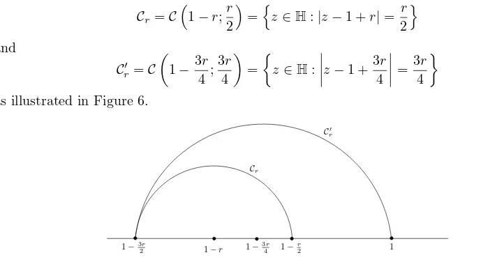
Theorem 1.1. Let x >0 be a fixed real number, and suppose0< ǫ≤x/3. If γ: [0,∞)→H We conclude with an application of Theorem 1.1 by combining it with a method due to Dub´edat [4]. For the remainder of the paper suppose that 4< κ <8; as before, leta= 2/κ. Suppose that 0< r≤1/3 and consider the two semicircles
Cr=C
Figure 6: The semicirclesC′
randCr.
r). From this we conclude that there exists a constantc′a such that
1−c′ar4a−1≤ inf z∈Cr
In order to derive an upper bound for the expression in (9), we use a method from Dub´edat [4]. We now outline this method referring the reader to that paper for further details. Letgtdenote
the solution to the chordal Loewner equation (4) with driving functionUt=−BtwhereBtis
a standard one-dimensional Brownian motion with B0 = 0. For t < T1, the swallowing time of the point 1, consider the conformal transformation ˜gt:H\Kt→Hgiven by
If we now perform the time-change
σ(t) =
then ˜gσ(t)(z) satisfies the stochastic differential equation
d˜gt(z) =
For ease of notation, and because it does not concern us at present, we have also denoted the time-changed flow by {g˜t(z), t ≥ 0}. Furthermore, it is shown in detail in [4] that for all
κ >0, the time-changed stochastic flow{g˜t(z), t≥0}given by (10) does not explode in finite
time a.s. Therefore, if F is an analytic function on Hsuch that{F(˜gt(z)), t≥0} is a local martingale, then Itˆo’s formula (att= 0) implies that F must be a solution to the differential equation
w(1−w)F′′(w) + [2a−(2−2a)w]F′(w) = 0. (11)
An explicit solution to (11) is given by
F(w) = Γ(2a) Γ(1−2a)Γ(4a−1)
Z w
0
ζ−2a(1−ζ)4a−2dζ (12)
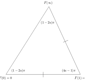
which is normalized so thatF(0) = 0 andF(1) = 1. Note that (12) is a Schwarz-Christoffel transformation of the upper half plane onto the isosceles triangle whose interior angles are (1−2a)π, (1−2a)π, and (4a−1)π. The boundary valuesF(0) = 0 andF(1) = 1 imply that two of the vertices of the triangle are at 0 and 1, and from (12) we conclude that the third vertex of the triangle is at
F(0) = 0 F(1) = 1
(1−2a)π (4a−1)π
(1−2a)π
F(∞)
Figure 7: The isosceles triangle with vertices at 0, 1, andF(∞).
from which it follows that ℜ(F(∞)) ≥ 0 and that |F(∞)−1| = 1 as is to be expected for this isosceles triangle. The image of H under F is illustrated in Figure 7. We now apply the optional sampling theorem to the martingale F(˜gt∧Tz∧T1(z)) to find (see the discussion
surrounding Proposition 1 of [4]) that forz∈H,
F(˜g0(z)) =F(z) =F(0)P{Tz< T1}+F(1)P{Tz=T1}+F(∞)P{Tz> T1}
=P{Tz=T1}+F(∞)P{Tz> T1}. (13)
Consequently, identifying the imaginary and real parts of the previous equation (13) implies that
ℜ{F(z)}=P{Tz=T1}+ℜ{F(∞)}P{Tz > T1}.
Since ℜ{F(∞)} ≥ 0, we conclude P{Tz = T1} ≤ ℜ{F(z)} ≤ |F(z)|. But now integrating
along the straight line from 0 toz (i.e., lettingθ= arg(z),ζ=ρeiθ, 0≤ρ≤ |z|) gives
|F(z)|= Γ(2a) Γ(1−2a)Γ(4a−1)
¯ ¯ ¯ ¯ ¯
Z |z| 0
(ρeiθ)−2a(1−ρeiθ)4a−2eiθdρ ¯ ¯ ¯ ¯ ¯
≤ Γ(2a)
Γ(1−2a)Γ(4a−1)
Z |z| 0
ρ−2a|1−ρ|4a−2dρ
= 1− Γ(2a)
Γ(1−2a)Γ(4a−1)
Z 1
|z|
ρ−2a(1−ρ)4a−2dρ
which relied on the fact that 4a−2<0. Ifz ∈ Cr so that 0<1−32r ≤ |z| ≤1−r2 <1 by
definition, then
Z 1
|z|
ρ−2a(1−ρ)4a−2dρ≥Z 1
|z|
(1−ρ)4a−2dρ= (1− |z|)4a−1
4a−1 ≥ 21−4a
4a−1r
4a−1.
Hence,
where
c′′a =
21−4a˜c a
4a−1 and ˜ca=
Γ(2a) Γ(1−2a)Γ(4a−1).
Taking the supremum of the previous expression over all z ∈ Cr gives us the required upper
bound to (9). Hence, we have proved the following theorem.
Theorem 6.1. Let 0< r≤1/3. If γ: [0,∞)→His a chordal SLEκ inHfrom 0 to∞ with 4< κ <8 anda= 2/κ, then there exist constants c′
a andc′′a such that
1−c′ar4a−1≤ inf z∈Cr
P{Tz=T1} ≤ sup z∈Cr
P{Tz=T1} ≤1−c′′ar4a−1
where
Cr=C
³
1−r;r 2
´
=nz∈H:|z−1 +r|= r 2
o
denotes the circle of radiusr/2 centred at1−rin the upper half plane as in (7). This theorem now yields the following corollary.
Corollary 6.2. Let 0< r≤1/3. Ifγ: [0,∞)→His a chordal SLEκ inHfrom 0 to∞ with 4< κ <8 anda= 2/κ, then there exist constants c′
a andc′′a such that
1−c′ar4a−1≤P{Tz=T1 for allz∈ Cr} ≤1−c′′ar4a−1
whereCr is given by (7) as above.
Proof. Letz0= 1−r+ir2 so thatz0∈ Cr. Theorem 6.1 implies that there exists a constant
c′′a such that
P{Tz=T1 for allz∈ Cr} ≤P{Tz0 =T1} ≤ sup
z∈Cr
P{Tz=T1} ≤1−c′′ar4a−1. (14)
As noted earlier, it follows from Theorem 1.1 thatP{γ[0,∞)∩ C′
r 6=∅} ≍r4a−1 where C′r is
given by (8), and so there exists a constantc′
a such that
P{Tz=T1 for allz∈ Cr} ≥P{γ[0,∞)∩ Cr′ =∅} ≥1−c′ar4a−1. (15)
Taking (14) and (15) together completes the proof.
Addendum
After this paper was completed, two preprints relevant to the subject at hand were released. Both Alberts and Sheffield [2] and Schramm and Zhou [11] prove, independently and using different methods, that for 4 < κ < 8 the SLEκ curve intersected with the real line has
Hausdorff dimension 2−8/κ a.s. Specifically, Alberts and Sheffield [2] establish an upper bound on the asymptotic probability of an SLEκ curve hitting two small intervals on the real
line as the interval width goes to zero, whereas Schramm and Zhou [11] examine how close the chordal SLEκ curve gets to the real line asymptotically far away from its starting point. In
Acknowledgements
This paper had its origins at the Workshop on Random Shapes held at the Institute for Pure & Applied Mathematics in March 2007, and was completed during the 2007 IAS/Park City Mathematics Institute on Statistical Mechanics. The authors would like to thank both orga-nizations for partial financial support, Peter Jones who organized the IPAM workshop, Scott Sheffield and Tom Spencer who organized the PCMI program, as well as Christophe Garban, Greg Lawler, and Ed Perkins who provided us with a number of valuable comments. Special thanks are owed to the anonymous referee who had many useful suggestions for clarifying the exposition.
References
[1] M. Abramowitz and I. A. Stegun, editors. Handbook of Mathematical Functions with Formulas, Graphs, and Mathematical Tables. National Bureau of Standards, Washington, DC, 1972. MR0757537
[2] T. Alberts and S. Sheffield. Hausdorff dimension of the SLE curve intersected with the real line. To appear,Electron. J. Probab.
[3] V. Beffara. The dimension of the SLE curves. To appear,Ann. Probab.MR2078552 [4] J. Dub´edat. SLE and triangles. Electron. Comm. Probab., 8:28–42, 2003. MR1961287 [5] C. Garban and J. A. Trujillo Ferreras. The expected area of the filled planar Brownian
loop isπ/5. Comm. Math. Phys., 264:797–810, 2006. MR2217292
[6] T. Kennedy. Monte Carlo Tests of Stochastic Loewner Evolution Predictions for the 2D Self-Avoiding Walk. Phys. Rev. Lett., 88:130601, 2003.
[7] G. F. Lawler. Conformally Invariant Processes in the Plane. American Mathematical Society, Providence, RI, 2005. MR2129588
[8] S. Rohde and O. Schramm. Basic properties of SLE. Ann. Math., 161:883–924, 2005. MR2153402
[9] O. Schramm. Scaling limits of loop-erased random walks and uniform spanning trees. Israel J. Math., 118:221–288, 2000. MR1776084
[10] O. Schramm. A percolation formula. Electron. Comm. Probab., 6:115–120, 2001. MR1871700
[11] O. Schramm and W. Zhou. Boundary proximity of SLE. Preprint available online at
![Figure 2: The event {γ′[0, tγ′] ∩ C(0; Rx) = ∅} in the 0 < κ ≤ 4 case.](https://thumb-ap.123doks.com/thumbv2/123dok/980631.915939/2.612.196.354.244.329/figure-event-g-tg-c-rx-k-case.webp)
![Figure 4: The event that γ[0, ∞) intersects the interval [x − rx, x + rx].](https://thumb-ap.123doks.com/thumbv2/123dok/980631.915939/6.612.106.443.253.335/figure-event-g-intersects-interval-x-rx-rx.webp)