E l e c t ro n i c
J o u r n
a l o
f P
r o b
a b i l i t y
Vol. 10 (2005), Paper no. 20, pages 691-717. Journal URL
http://www.math.washington.edu/∼ejpecp/
Quadratic Variations along Irregular Subdivisions for Gaussian Processes
Arnaud Begyn
LSP, Universit´e Paul Sabatier, 118 route de Narbonne 31062 TOULOUSE Cedex 04, FRANCE
E-mail: [email protected], http://www.lsp.ups-tlse.fr/Fp/Begyn/
Abstract
In this paper we deal with second order quadratic variations along general subdivi-sions for processes with Gaussian increments. These have almost surely a deterministic limit under conditions on the mesh of the subdivisions. This limit depends on the sin-gularity function of the process and on the structure of the subdivisions too. Then we illustrate the results with the example of the time-space deformed fractional Brownian motion and we present some simulations.
AMS MSC (2000): primary 60F15; 60G15; secondary 60G17; 60G18
1
Introduction
In 1940 Paul L´evy (see [17]) proves that if W is the Brownian motion on [0,1] then:
lim
n→+∞
2n X
k=1
·
W
µ
k 2n
−W
µ
k−1 2n
¶¸2
= 1, a.s..
Then in [2] and in [11] this result is extended to a large class of processes with Gaussian increments. In these cases the subdivisions are regular and the mesh is fixed (equal to 1/2n).
More general subdivisions are used later in [10] and [15]. The subdivisions can be irregular and the optimal condition is that the mesh must be at most o(1/logn).
In the case of the fractional Brownian motion, the quadratic variation is used to construct some estimators of the Hurst index H. But these estimators are not asymptotically normal when H > 3/4 (see [12]). To solve this problem in [14], [3], [8] and [9] authors introduce generalized quadratic variations. The most common variation is the second order quadratic variation, which will be defined in the next section. But one more time subdivisions are regular.
In this paper we extend the theorem of [9] to a large class of subdivisions which may be irregular. We obtain that the limit of the second order quadratic variation depends on the structure of the sequence of subdivisions, and one more time that the mesh must be at most o(1/logn).
In the first section we state our notations. In the second one we prove our theorem. The third one is a discussion about the assumptions made on the structure of the subdivisions. In the fourth one we apply the results to the example of the time-space deformed fractional Brownian motion. In the last one we illustrate the examples with some simulations.
2
Notations
Let (Xt)t∈[0,1] be a square integrable process. We can define its mean function:
∀t ∈[0,1], Mt =EXt,
and its covariance function:
∀s, t∈[0,1], R(s, t) =E¡(Xt−Mt) (Xs−Ms)¢.
We define the second order increments ofR too: δh1,h2
1 R(s, t) = h1R(s+h2, t) +h2R(s−h1, t)−(h1+h2)R(s, t),
δh1,h2
Let (πn)n∈N be a sequence of subdivisions of the interval [0,1]. One denotes by Nn the number of subintervals of [0,1] generated by πn. We suppose that πn can be written:
πn =
n
t(0n) = 0 < t(1n) <· · ·< t(Nnn) = 1o,
One sets theupper mesh of πn:
mn = max{t(in+1) −t (n)
i ; 0≤i≤Nn−1},
and the lower mesh:
pn= min{t(in+1) −t (n)
i ; 0≤i≤Nn−1}.
Note that one has:
∀n∈N, pn≤ 1
Nn ≤
mn.
Definition 1. We say that the sequence of subdivisions(πn)n∈N is regular if we have: ∀n∈N, mn=pn = 1
Nn
.
Or equivalently:
∀n∈N,∀k ∈ {0;. . .;Nn}, t(n)
k =
k Nn
.
For fractional processes the following second order quadratic variation has been used:
Sπn(X) =N
1−γ n
NXn−1
k=1
h
Xk+1
Nn +X k−1
Nn −2X k Nn
i2
, (1)
which is taken along the regular subdivision with mesh 1/Nn. The real numberγ is in ]0,2[
and depends on the regularity of the process, as we will see later.
Iff : [0,1]7−→R is of class C2 in a neighborhood of the point t then the Taylor formula
yields:
lim
h→0
f(t+h) +f(t−h)−2f(t)
h2 =f
′′(t). (2)
This motivates the termXk+1
Nn +X k−1
Nn −2X k
Nn in (1). If we want to use irregular
subdi-visions we must generalize (2). One more time the Taylor formula yields:
lim
h1→0
h2→0
h1f(t+h2) +h2f(t−h1)−(h1+h2)f(t)
h1h2(h1+h2)
= 1 2f
′′(t).
So one defines the second order increments of X:
where (we drop the super-index int(kn) whenever it is possible): ∆tk=tk+1−tk, k = 0, . . . , Nn−1.
We will see later thatE£(∆Xk)2¤ is asymptotically of the same order as:
(∆tk−1)
3−γ
2 (∆t
k)
3−γ
2 (∆t
k−1+ ∆tk).
That is why we define the second order quadratic variation of X along a general subdi-vision by:
Vπn(X) = 2
NXn−1
k=1
(∆tk) (∆Xk)2
(∆tk−1)
3−γ
2 (∆t
k)
3−γ
2 (∆t
k−1+ ∆tk)
(3)
where γ ∈]0,+∞[.
Note that when the sequence (πn)n∈N is regular, one has: Vπn(X) = Sπn(X).
Let us recall the Landau notations. Let (un)n∈N and (vn)n∈N be two sequences of real numbers such that ∀n, vn6= 0. We will say that:
(i) un
n→+∞
= O(vn) if the sequence (un/vn)n∈N is bounded, (ii) un
n→+∞
= o(vn) if the sequence (un/vn)n∈N goes to zero when n→+∞.
To study the almost sure convergence ofVπn(X) we will use the following assumption on
the sequence (πn)n∈N.
Definition 2. Let(lk)1≤k be a sequence of reals in the interval]0,+∞[. We say that(πn)n∈N
is a sequence of subdivisions with asymptotic ratios(lk)1≤k if it satisfies the following
assump-tions:
1.
mn
n→+∞
= O(pn). (4)
2.
lim
n→+∞1≤ksup≤Nn−1
¯ ¯ ¯ ¯ ¯
∆t(kn−)1 ∆t(kn) −lk
¯ ¯ ¯ ¯
¯= 0. (5)
The set L={l1;l2;. . .;lk;. . .}will be called the range of the asymptotic ratios of the sequence
It is clear that if the sequence (πn)n∈N is regular, then it is a sequence with asymptotic ratios (lk)1≤k where: ∀k ≥1, lk= 1.
Note that assumption (4) implies:
∃K >0,∀n ∈N, pn≤ 1
Nn ≤
mn≤Kpn, (6)
therefore (lk)1≤k⊂[1/K, K], and the closure of L in ]0,+∞[ is compact.
In the sequel we only consider process with Gaussian increments.
Definition 3. A process (Xt)t∈[0,1] has Gaussian increments if, for any subdivision {t0 =
0< t1 <· · ·< tN = 1} of [0,1], the random vector (Xti+1−Xti)0≤i≤N−1 is Gaussian.
In the proof of the next section we use the following notations:
djk =E(∆Xj∆Xk), j, k = 1, . . . , Nn−1. (7)
And:
µk= (∆tk−1)
3−γ
2 (∆t
k)
3−γ
2 (∆t
k−1+ ∆tk), k= 1, . . . , Nn−1 (8)
We remark that:
∀1≤k ≤Nn−1,
2p4
n
mγn ≤
µk ≤
2m4
n
pγn
. (9)
3
The results
We prove the almost sure convergence of Vπn(X) to a deterministic limit under some
conditions on the covariance function of the process X and on the mesh of the subdivisions πn.
For a functiong :]0,+∞[×]0,1[→R we need the following assumption of continuity:
∀ǫ >0,∃δ >0; ∀l ∈ L,∀t, t∗ ∈]0,1[, |t−t∗|< δ =⇒ |g(l, t)−g(l, t∗)|< ǫ. (10) Theorem 4. Let (πn)n∈N be a sequence of subdivisions with asymptotic ratios (lk)1≤k and
range of the asymptotic ratiosL. Let (Xt)t∈[0,1] be a square integrable process, with Gaussian
increments, verifying:
1. t7−→Mt =EXt has a bounded first derivative on [0,1],
2. the covariance function R(s, t) has the following properties:
(b) the derivative ∂s∂24∂tR2 exists and is continuous on ]0,1]2\{s = t}, and there exists
tion (10) and such that:
∀ǫ >0,∃δ >0, sup
and such that the following limit exists and is finite:
lim
3. The lower mesh of the subdivisions πn satisfy:
pn n→=+∞o
Then one has almost surely:
lim
(i)If assumptions (11), (12) is satisfied for γ0 then they are satisfied for all γ > γ0 too,
but the corresponding function gγ is equal to zero. Whenγ0 is chosen as the infimum of real
satisfying (11) and (12), gγ0 can be viewed as a generalization of the singularity function of
X (see [2]).
(ii) As we will see later, in most cases one is able to compute explicitly the limit
limn→+∞
R1
0 g(ln(t), t)dt.
(iii)We assume that the covariance function has a singularity on the set{s= 0}∪{t= 0}
Proof of theorem 4. Along the proof K denotes a generic positive constant, whose value does not matter.
First we assume that the theorem is true in the case of X centered. Because of assumption 1., one has whenn →+∞:
which comes from (6),(9) and assumption 1.
IfX is not centered, one setsXet=Xt−Mt. Using Baxter’s arguments (see [2]) and (16)
one has:
lim
n→+∞Vπn(X) = limn→+∞Vπn(X)e a.s..
However the theorem is true in the case ofX not centered too. So one can assume that the process X is centered without loss of generality.
First we study the asymptotic properties ofEVπn(X). One remarks that:
djk =
Moreover assumptions (12) and (5) yield:
Assumption (10) implies:
This with (19) and (6) yield:
lim sup
Hence the proof is reduced to verify: a.s. lim
n→+∞(Vπn(X)−
EVπ
n(X)) = 0.
From Borel-Cantelli lemma, it is enough to find one sequence of positive real (ǫn)n∈N satisfying:
For that, we will proceed like in [15] and use Hanson and Wright’s bound (see [13]). One remarks thatVπn(X) is the square of the Euclidean norm of one (Nn−1)-dimensional
Gaussian vector which components are:
s
2∆tk
µk
∆Xk, 1≤k ≤Nn−1.
So by the classical Cochran theorem, one can find an nonnegative real numbers
(λ1,n, . . . , λan,n) and one an-dimensional Gaussian vector Yn, such that its components are
independent Gaussian variables N(0,1) and:
Vπn(X) =
an
X
j=1
λj,n(Yn(j))2. (23)
Then the Hanson and Wright’s inequality yields:
where A1, A2 are nonnegative constants, λ∗n is defined by λ∗n= sup1≤j≤anλj,n.
Therefore, the inequality (24) becomes :
∀1≥ǫ >0, P(|Vn−EVn| ≥ǫ)≤2 exp
symmetric matrix. We note λmax its higher eigenvalue. Then one has:
λmax ≤ max
This with inequality (9) yield:
λ∗n ≤ 2 max
So one must study the asymptotic properties of the djk. For that we proceed in three
steps, according to the value of k−j.
If f :]0,1] 7−→ R is a two times differentiable function one has for 0 < h1 < t and
Here one uses assumption (11) which yields:
¯
And on the integration set one has:
|w−z| ≥tj−1−tk+1 =
Using the same techniques as above one gets forǫ near 0+:
|d(jkǫ)| ≤ 4Cm
6
n(1−ǫ)2
((j−k−2)pn−2ǫmn))γ+2
One makesǫ tends to 0+ in this inequality. It yields that (29) is still true when j = 1 or
Thanks to (6) one gets the following estimate: max
So the preceding three steps and (26) yield:
λ∗n n→=+∞O(pn). (30)
Hence (25) and the preceding estimates yield for 0< ǫ≤1:
P(|Vn−EVn| ≥ǫ)≤2 exp
So conditions (22) are satisfied.
✷
Now we give briefly two cases where the limit (13) exists and can be easily computed. (C1) If g is invariant on L, i.e. ∀t ∈ [0,1],∀l, l∗ ∈ L, g(l, t) = g(l∗, t). Then it is clear that
(13) is satisfied. Indeed:
NXn−1
(C2) If the sequence of functions (ln(t))n∈N converges uniformly to l(t) on the interval [0,1], then:
thanks to the Riemann theorem. So assumption (13) is fulfilled.
4
Construction of irregular sequences of subdivisions
We give a necessary and sufficient condition to find a sequence of subdivisions (πn)n∈N which has a given sequence of asymptotic ratios (lk)k≥1 ⊂]0,+∞[ .
Proposition 5. Let (lk)k≥1 be a sequence of real numbers in ]0,+∞[ and (Nn)n∈N be an
increasing sequence of positive integer numbers such that:
∃D >1,∀L∈N∗, 1
Then (lk)k≥1 is the sequence of asymptotic ratios of a sequence of subdivisions
³
πn=
n
t(0n) = 0< t1(n)<· · ·< t(Nnn)= 1o´
n∈N. This sequence is unique under the condition:
∀1≤k ≤Nn−1, lk =
∆t(kn−)1
∆t(kn). (34)
The converse is true: if (πn)n∈N is a sequence of subdivisions, (Nn)n∈N is the associated
sequence of number of subintervals and (lk)k≥1 is the sequence of the asymptotic ratios of
(πn)n∈N, then the sequences (lk)k≥1 and (Nn)n∈N satisfy the conditions (32) and (33).
Therefore: satisfying conditions (32) and (33).
For n ∈ N, we define the subdivision πn = nt(n)
One gets a sequence of subdivisions with asymptotic ratios (lk)k≥1. Indeed:
∀1≤k ≤Nn−1,
∆t(kn−)1 ∆t(kn) =lk, so the sequence satisfies (5).
We note kn and jn the integer such that:
and because of (32):
Second case: kn < jn. We use the same arguments. One has:
mn
pn
=
jYn−1
i=kn
li =
Pjn−1
Pkn−1
≤D2.
Third case: kn =jn. Then:
mn
pn
= 1 ≤D2. Hence in all cases:
mn
pn ≤
D2,
so the sequence (πn)n∈N satisfies (4) too.
Now we must show the unicity of (πn)n∈N under the assumptions of the proposition. Necessarily one has PNn−1
k=0 ∆t
(n)
k = 1 which yields:
Ã
1 +
NXn−2
j=1
NYn−1
i=j+1
∆t(in−)1 ∆t(in)
!
∆t(Nnn)−1 = 1.
With (34) one gets: Ã 1 +
NXn−2
j=1
NYn−1
i=j+1
li
!
∆t(Nnn)−1 = 1. (35)
And with (35) and (34), one gets the recursive procedure used to define (πn)n∈N. Since this procedure defines a unique sequence, (πn)n∈N is the unique solution of our problem.
✷
Example. One sets Nn =n and lk = 1 + k12. Note that the sequence (PL) is increasing
and lower bounded by 1. So condition (32) is satisfied with D=Q+j=1∞³1 + j12
´
. Moreover:
NYn−1
i=j
li ≥lj = 1 +
1 j2 ≥1,
so condition (33) is satisfied too.
5
Example: time-space deformed fractional Brownian
motion
5.1
The fractional Brownian motion
The fractional Brownian motion (FBM) with Hurst’s index H ∈]0,1[ is the centered Gaussian process ¡BH
t
¢
t∈R, vanishing at the origin, with covariance function given by: ∀s, t ∈R, R(s, t) = Cov¡BH
s , BtH
¢
= 1 2
¡
|s|2H +|t|2H − |s−t|2H¢.
ForH = 1/2, ¡BH t
¢
t∈R is the Brownian motion. The process BH is self-similar with index H:
∀ǫ >0,©BH(ǫt);t∈Rª (=L)©ǫHBH(t);t∈Rª,
and its increments are stationary.
Moreover the H¨older critical exponent of its sample paths is equal to H (see [1] th.8.3.2 and th.2.2.2 ), in the following sense:
Definition 6. Let β ∈]0,1[. A process (Xt)t∈R is said to have H¨older critical exponent β
whenever it satisfies the two following properties:
• for any β∗ ∈]0, β[, the sample paths of X satisfy a.s. a uniform H¨older condition of
order β∗ on any compact set, i.e; for any compact set K of R, there exists a positive
r.v. A such that a.s.:
∀s, t ∈K,|Xs−Xt| ≤A|s−t|β
∗
;
• for any β∗ ∈]β,1[, a.s. the sample paths of X fails to satisfy any uniform H¨older
condition of order β∗.
In [9] authors proved that almost surely:
lim
n→+∞n
2H−1
n−1
X
k=1
h
BHk+1
n +B
H
k−1
n −2B
H
k n
i2
= 4−22H. (36)
We are able now to sharpen this result. Let (πn)n∈N be a sequence of subdivisions with asymptotic ratios (lk)k≥1.
On the one hand we compute the derivative ∂4R
∂s2∂t2. One has:
∀s, t ∈]0,1]2\{s=t}, ∂
4R
∂s2∂t2(s, t) =
where γ = 2−2H.
So (11) is satisfied withC = 2H(2H−1)(2H−2)(2H−3).
On the other hand we must compute the singularity function ofBH. We use the notations
of the theorem 4. One has:
³
The functionφis continuous on ]0,+∞[, so it is uniformly continuous on compact subsets of ]0,+∞[. This property proves the limit (12). Moreover it is obvious that g satisfies assumption (10). Therefore theorem 4 can be applied to BH.
By example, for a regular sequence of subdivisions one has a.s.:
lim
We give as well an example of non regular subdivision. We set: Nn = 2n,
This is a sequence of subdivisions with asymptotic ratios (lk)1≤k where:
∀k ≥1, l2k = 2,
∀k ≥0, l2k+1 =
Its range of asymptotic ratios isL ={1/2; 2}andg(l, t) is invariant inlon this set (which is condition (C1)), so one is able to compute the limit (13). Therefore theorem 4 yields:
lim
n→+∞Vπn(B
H) = 1 + 22H−1−32H−1
2H−3/2 . (39)
Note that when H 6= 1/2, the value of this limit is different from (38). Indeed its depends not only on the singularity function of the process but on the asymptotic ratios of the subdivisions too.
ForH = 1/2 the singularity functiong does not more depend on l. Indeed: ∀t∈]0,1[,∀l ∈]0,+∞[, g(l, t) = 2.
It is classical that the standard quadratic variation of the Brownian motion does not depend on the sequence of subdivisions; we obtain the same result for the second order quadratic variation.
5.2
Time-space deformed fractional Brownian motion
Let σ and ω be two functions from R to R. We define the (σ, ω)-time-space deformed
fractional Brownian motion (ZH
t )t∈R by the formula:
∀t∈R, ZtH =σ(t)BH(ω(t)). (40)
This is a centered Gaussian process with covariance function:
∀s, t ∈R,E(ZsHZtH) = σ(s)σ(t)
2
¡
|ω(s)|2H +|ω(t)|2H − |ω(s)−ω(t)|2H¢.
We want to study this process in the following way: does it have the same properties as the FBM? It is clear that it has no more stationary increments. In the sequel, we study its properties of self-similarity and H¨older regularity, and we apply theorem 4 to this process.
The following lemma will be useful:
Lemma 7. Let I, J, K be three subintervals of R and α, β two real numbers in [0,1]. We
will say that a function f :I −→J is α-H¨olderian on I if:
∃K >0,∀x, y ∈I,|f(x)−f(y)| ≤K|x−y|α.
1. Let f :I −→J and g : I −→ K be two functions. Assume that f is α-H¨olderian and bounded on I, andg isβ-H¨olderian and bounded onI. Then the function f g :I −→R
is min(α, β)-H¨olderian.
2. Let f :I −→J and g :J −→K be two functions. Assume that f is α-H¨olderian an g
¿From this lemma we can deduce immediately the regularity of the sample paths of ZH.
Proposition 8. We assume that σ is Σ-H¨olderian and ω is Ω-H¨olderian on a compact interval I of R with Σ,Ω ∈ [0,1]. Then for all H′ < H the sample paths of ZH are a.s.
min(Σ,ΩH′)-H¨olderian on I.
Proof of proposition 8. It is a straightforward consequence of lemma 7.
✷
Now we show a property of self-similarity of the processZH. We begin with the definition
of this property (see [4]) in the case of a Gaussian field.
Definition 9. Let d ∈ N∗ and β > 0. A process (X(t))t∈Rd is locally asymptotically self-similar (l.a.s.s.) of order β at point t0 ∈ Rd if the finite dimensional distributions of the
field ½
X(t0+ǫt)−X(t0)
ǫβ ;t ∈R d
¾
converge to the finite dimensional distributions of a non trivial Gaussian field when ǫ→0+.
The limit field is called the tangent field at point t0.
We give assumptions on the functions σ, ω so that the process ZH is l.a.s.s..
Proposition 10. Let t0 ∈R and Σ∈]H,1]. Assume that:
1. ω is differentiable at point t0 and ω′(t0)6= 0,
2. σ is Σ-H¨olderian on a neighborhood of t0 and σ(t0)6= 0.
Then the process ZH is l.a.s.s. at point t
0 of order H and the tangent process is:
³
T(t0)
t
´
t∈R=σ(t0)|ω
′(t
0)|H
¡
BtH
¢
t∈R.
Remark.
Under these assumptions proposition 8 yields that for all H′ < H the sample paths of ZH are
a.s. H′-H¨olderian. Proposition 10 yields that they are not H′-H¨olderian in the neighborhood
of t0 for all H′ > H. Therefore the H¨older critical exponent of ZH is equal to H.
Proof of proposition 10. Along the proof K will denote a generic positive constant, whose value does not matter.
Let t0 ∈R. We denote by R (resp. ρ) the covariance function of the process ZH (resp.
BH). Since we work with centered Gaussian process it is enough to show that:
∀s, t ∈R, lim
ǫ→0+
1 ǫ2HCov
¡
ZH(t
0+ǫs))−ZH(t0), ZH(t0+ǫt)−ZH(t0)
¢
One sets for h1, h2 >0:
Λh1,h2R(t
0) =R(t0+h1, t0+h2)−R(t0+h1, t0)−R(t0, t0+h2) +R(t0, t0).
Equality (41) is equivalent to:
∀s, t∈R, lim
ǫ→0+
Λǫs,ǫtR(t
0)
ǫ2H =σ(t0)
2|ω′(t
0)|2Hρ(s, t). (42)
One takes s, t∈R. One has:
R(s, t) = σ(s)σ(t) 2
¡
|ω(s)|2H +|ω(t)|2H − |ω(s)−ω(t)|2H¢.
Therefore:
Λǫs,ǫtR(t0) =
σ(t0+ǫs)σ(t0+ǫt)
2
¡
|ω(t0+ǫs)|2H +|ω(t0+ǫt)|2H − |ω(t0+ǫs)
−ω(t0+ǫt)|2H
¢
−σ(t0+ǫs)σ(t0) 2
¡
|ω(t0+ǫs)|2H +|ω(t0)|2H − |ω(t0+ǫs)−ω(t0)|2H
¢
−σ(t0+2ǫt)σ(t0)¡|ω(t0+ǫt)|2H +|ω(t0)|2H − |ω(t0+ǫt)−ω(t0)|2H
¢
+σ(t0)2|ω(t0)|2H.
One sets:
Λǫs,ǫtR(t0) = Φ1(ǫ) + Φ2(ǫ),
where:
Φ1(ǫ) =
σ(t0+ǫt)−σ(t0)
2
¡
|ω(t0+ǫs)|2Hσ(t0+ǫs)− |ω(t0)|2Hσ(t0)
¢
+σ(t0+ǫs)−σ(t0) 2
¡
|ω(t0+ǫt)|2Hσ(t0+ǫt)− |ω(t0)|2Hσ(t0)
¢
,
and:
Φ2(ǫ) =
σ(t0+ǫs)σ(t0)
2 |ω(t0+ǫs)−ω(t0)|
2H
+σ(t0+ǫt)σ(t0)
2 |ω(t0+ǫt)−ω(t0)|
2H
−σ(t0+ǫt)σ(t2 0+ǫs)|ω(t0+ǫt)−ω(t0+ǫs)|2H.
First we show that:
lim
ǫ→0+
Φ1(ǫ)
ǫ2H = 0. (43)
By assumption σ is Σ-H¨olderian on a neighborhood of t0 and ω is differentiable at t0, so
is min(1,2H)-H¨olderian on a neighborhood oft0. Therefore lemma 7 allows us to conclude
that the function x7→ |ω(x)|2Hσ(x) is min(Σ,2H)-H¨olderian on a neighborhood of t
0.
Hence there existsK >0 such that for ǫ enough small: |Φ1(ǫ)| ≤KǫΣ+min(Σ,2H).
Moreover one has assumed that Σ> H, so Σ + min(Σ,2H)>2H. This shows (43). Now we show that:
lim
ǫ→0+
Φ2(ǫ)
ǫ2H =σ(t0)
2|ω′(t
0)|2Hρ(s, t). (44)
Ifs= 0 or t= 0 equality (44) is obvious. So one can assume that s6= 0 and t6= 0. Since ω is differentiable at point t0 one has:
lim
ǫ→0+
|ω(t0+ǫs)−ω(t0)|2H
ǫ2H = s
2H|ω′(t
0)|2H,
lim
ǫ→0+
|ω(t0+ǫt)−ω(t0)|2H
ǫ2H = t
2H|ω′(t
0)|2H,
lim
ǫ→0+
|ω(t0+ǫs)−ω(t0+ǫt)|2H
ǫ2H = |s−t|
2H|ω′(t
0)|2H.
This shows equality (44). Since (43) and (44) are sufficient conditions for (42) the propo-sition is proved.
✷
Now we apply theorem 4 in order to generalize previous results about the FBM. We make additional assumptions on σ and ω.
Proposition 11. Assume that:
1. σ is of class C3 and ω of class C2 on [0,1],
2. ω(0)≥0,
3. inft∈[0,1]ω′(t) = β >0.
Let(πn)n∈N be a sequence of subdivisions with asymptotic ratios(lk)k≥1. Assume too that:
pn n→=+∞o
µ
1 logn
.
Then theorem 4 can be applied to ZH with γ = 2−2H and:
g(l, t) = σ(t)2|ω′(t)|2H1 +l
2H−1−(1 +l)2H−1
Proof of proposition 11. Along the proofK denotes a generic positive constant, whose value does not matter.
We denote by R the covariance function of ZH. One has:
R(s, t) = σ(s)σ(t) 2
¡
|ω(s)|2H +|ω(t)|2H − |ω(s)−ω(t)|2H¢.
We must show that the assumptions of theorem 4 are satisfied. For 1 and 2.(a) it is obvious.
For assumption 2.(b): since ∀t > 0, ω(t) > ω(0) = 0 and ∀s 6= t, ω(s) 6= ω(t) it is clear that ∂s∂24∂tR2 exists and is continuous on ]0,1]2\{s=t}.
Moreover the functions σ, ω and their first and second derivatives are bounded on [0,1]. The computation of ∂s∂24∂tR2 shows that there exists K >0 such that:
∀s, t ∈]0,1]2\{s=t},
¯ ¯ ¯ ¯
∂4R
∂s2∂t2(s, t)
¯ ¯ ¯
¯≤K
X
i∈I
¡
|ω(s)|2H−i1+|ω(t)|2H−i2 − |ω(s)−ω(t)|2H−i3¢,
where i= (i1, i2, i3) and I is a subset of {0; 1; 2; 3; 4}3.
The functions (s, t)7→ |s−t|2+γ|ω(s)|2H−i1 and (s, t)7→ |s−t|2+γ|ω(t)|2H−i2 are bounded
on ]0,1]2\{s=t} since they are continuous on [0,1]2.
Likewise (s, t)7→ |s−t|2+γ|ω(s)−ω(t)|2H−i3 is bounded on ]0,1]2\{s=t}when 2H−i
3 ≥
0.
If 2H−i3 <0 one uses the assumption onω′. One gets:
∀s, t∈[0,1],|ω(s)−ω(t)| ≥β|s−t|, and consequently:
∀s, t ∈]0,1]2\{s=t},|ω(s)−ω(t)|2H−k≤β2H−k|s−t|2H−k. Moreover there exists K >0 such that:
∀s, t ∈]0,1]2\{s=t},|s−t|2H−k ≤ K |s−t|2+γ.
Therefore assumption 2.(b) is fulfilled.
Now we verify assumption 2.(c). For f : [0,1]−→R one sets:
∆h1,h2f(t) =h
1f(t+h2) +h2f(t−h1)−(h1+h2)f(t),
Letǫ >0. We takeEδ for a δ >0 as in theorem 4. One sets for (l, t)∈]0,+∞[×]0,1[:
g1(l, t) = 0,
g2(l, t) = σ(t)2|ω′(t)|2Hl2H−1,
g3(l, t) = σ(t)2|ω′(t)|2H,
g4(l, t) = σ(t)2|ω′(t)|2H(1 +l)2H−1
Firstly we show that:
∃δ1 >0,sup
Eδ1
|Ψ1(h1, h2, t)−g1(l, t)| ≤ǫ. (46)
Applying Taylor formula it is easy to see that the term ∆λh(1+1,λhλ1)σh(3t)
1 is uniformly bounded
onEδfor all δ >0 (thanks to the facts thatσ isC3 andLhas a compact closure in ]0,+∞[).
Moreover, since L has a compact closure and σ|ω|2H is continuous, there exists K >0 such
that ∀0< δ <1:
∆h1,λh1(σ|ω|2H)(t)
hH1 −1/2 ≤Kh
3/2−H
1 on Eδ.
This proves (46). Secondly we prove: ∃δ2 >0,sup
Eδ2
|Ψ2(h1, h2, t)−g2(l, t)|+ sup
Eδ3
|Ψ3(h1, h2, t)−g3(l, t)|
+ sup
Eδ4
|Ψ4(h1, h2, t)−g4(l, t)| ≤ǫ. (47)
Likewise Taylor formula and compacity of the closure ofL imply that the terms
ω(t+λh1)−ω(t)
λh1 ,
ω(t−h1)−ω(t)
h1 and
ω(t+h2)−ω(t−λh2)
(1+λ)h2 have for limit ω
′(t) on E
δ. Then use the fact
that σ and x 7→ |x|2H are uniformly continuous on compact sets and ω is of class C2. One
gets (47).
Then (46) and (47) imply that assumption (12) is fulfilled withg(l, t) = lH−11/2 (g1(l, t)
+g2(l, t) +g3(l, t) +g4(l, t)). This function satisfies (10) thanks to the compacity of L and
the uniform continuity of σ|ω|2H.
Therefore assumption 2.(c) is fulfilled.
✷
Example: the fractional Ornstein-Uhlenbeck process. We consider the Lamperti transform (see [16]) of the FBM: we take σ(t) =e−λt and ω(t) =αeλt
H where λ, α >0. This
new process is stationary. If H = 1/2 it is the Ornstein-Uhlenbeck process with parameters √
If one uses proposition 11 one gets that the singularity function of the process OH is
Like in the case of the FBM it yields a strongly consistent estimator of the parameterH given by:
In the last section we illustrate the result obtained about the FBM with some simulations.
6
Simulations
We illustrate the results with some simulations in the case of the FBM. To simulate the FBM we use the method of the circulant matrix (see [5] and [7]) and Matlab°c. We use
two sequences of subdivisions: the first one is regular and the second one is not (we use the irregular sequence defined in section 5.1). If one uses the method of the circulant matrix to simulate the FBM one obtains a discretized path along a regular subdivision. Therefore for simulations we use the fact that the irregular sequence of section 5.1 can be refined in a regular sequence of subdivisions.
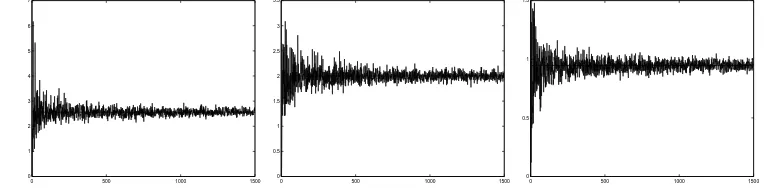
On figure 1 we have represented the values of Vπn(B
H) against the values of n, when
grows up to 1500, in the case of a regular sequence of subdivisions. We have made this for three values of H: 0.3, 0.5 and 0.8. On the figure we can see the convergence of Vπn(B
H)
claimed by (38). The value of the limit is respectively equal to 2.4843, 2 and 0.9686.
On figure 2 we have replaced the sequence of regular subdivisions with the irregular sequence constructed in section 5.1. Its range of asymptotic ratios is L ={1/2; 2}. On the figure we can see the convergence of Vπn(B
H) claimed by (39). The value of the limit is
respectively equal to 2.5581, 2 and 0.9463.
Figure 3 represents the histograms of the value of Vπn(B
H) for 1500 simulations with
n = 1500 andH = 0.3, 0.5 and 0.8, in the case of a regular sequence of subdivisions. In each case the mean is respectively equal to 2.4821, 1.9986 and 0.9659, and the standard deviation is equal to 0.1192, 0.0912 and 0.0393.
200 400 600 800 1000 1200 1400
200 400 600 800 1000 1200 1400 0
200 400 600 800 1000 1200 1400 0
the subdivisions are regular.
0 500 1000 1500
0
0 500 1000 1500
0
0 500 1000 1500
0
the subdivisions are irregular with range of asymptotic ratios equal to L={1/2; 2}.
1 1.5 2 2.5 3 3.5 4 4.5
Figure 3: Histograms of 1500 simulations ofVπn(B
H) forH = 0.3, 0.5 and 0.8 whenn= 1500
and the subdivisions are regular.
1 1.5 2 2.5 3 3.5 4 4.5
Figure 4: Histograms of 1500 simulations ofVπn(B
H) forH = 0.3, 0.5 and 0.8 whenn= 1500
We can see on all the histograms thatVπn(B
H) seems to be asymptotically normal. We know
it for the case of the FBM and regular subdivisions. We will try to show it in the general case in a future paper.
References
[1] A. Adler. The geometry of random fields. Ed. John Wiley and Sons, 1981.
[2] G. Baxter. A strong limit theorem for Gaussian processes. Proc. Amer. Soc., 7:522–527, 1956.
[3] A. Benassi, S. Cohen, J. Istas, and S. Jaffard. Identification of filtered white noises.
Stoch. Prob. Appl., 75:31–49, 1998.
[4] A. Benassi, S. Jaffard, and D. Roux. Elliptic Gaussian random processes. Rev. Math. Iboamerica, 13:7–18, 1997.
[5] G. Chan and A.T.A. Wood. Simulation of a stationary Gaussian process in [0,1]d.
Journ. of Comput. and Graph. Statistics., 3:409–432, 1994.
[6] P. Cheredito, H. Kawaguchi, and M. Maejima. Fractional Ornstein-Uhlenbeck processes.
Elect. Journ. of Proba., 8(3):1–14, 2003.
[7] J.F. Coeurjolly. Inf´erence statistique pour les mouvements Brownien fractionnaires et multifractionnaires. (French). PhD thesis, Universit´e Joseph Fourier Grenoble I., 2000. [8] J.F. Coeurjolly. Estimating the parameters of a fractional Brownian motion by discrete
variations of its sample paths. Stat. Inference Stoch. Process., 4(2):199–227, 2001. [9] S. Cohen, X. Guyon, O. Perrin, and M. Pontier. Singularity functions for fractional
processes, and application to fractional Brownian sheet.To appear in Annales de l’I.H.P.
[10] R.M. Dudley. Sample functions of the Gaussian process. Ann. Probability, 1:66–103, 1973.
[11] E.G. Gladyshev. A new limit theorem for stochastic processes with Gaussian increments.
Theor. Prob. Appl., 6(1):52–61, 1961.
[12] X. Guyon and J. Le´on. Convergence in law of the H-variations of a stationary Gaussian process in R. Ann. Inst. H. Poincar´e Probab. Statist., 25(3):265–282, 1989.
[13] D.L. Hanson and F.T. Wright. A bound on tail probabilities for quadratic forms in indepedent random variables. Ann. Math. Statist., 42:1079–1083, 1971.
[15] R. Klein and E. Gine. On quadratic variations of processes with Gaussian increments.
Annals of Probability., 3(4):716–721, 1975.
[16] J.W. Lamperti. Semi-stable stochastic processes. Trans. Amer. Math. Soc., 104:62–78, 1962.