A new approach to the modeling of financial volumes
Guglielmo D’AmicoDepartment of Pharmacy, University ”G. d’Annunzio” of Chieti-Pescara e-mail: [email protected]
Filippo Petroni
Department of Economy and Business, University of Cagliari, Cagliari
Abstract
In this paper we study the high frequency dynamic of financial volumes of traded stocks by using a semi-Markov approach. More precisely we assume that the intraday logarithmic change of volume is described by a weighted-indexed semi-Markov chain model. Based on this assumptions we show that this model is able to reproduce several empirical facts about volume evolution like time series dependence, intra-daily periodicity and volume asymmetry. Results have been ob-tained from a real data application to high frequency data from the Italian stock market from first of January 2007 until end of December 2010.
Keywords semi-Markov; high frequency data; financial volume
1
Introduction
Studies on market microstructure have acquired a crucial importance in order to explain the price formation process, see e.g. De Jong and Rindi (2009). The main variables are (logarithmic) price returns, volumes and duration. Sometimes they are modeled jointly and the main approach is the so-called econometric analysis, see e.g. Manganelli (2005) and Podobnik et al. (2009) and the bibliography therein.
The volume variable is very important not only because it interacts di-rectly with duration and returns but also because a correct specification of forecasted volumes can be used for Volume Weighted Average Price trading, see e.g. Brownlees et al. (2011). This variable has been investigated for long time and several statistical regularities have been highlighted, see e.g. Jain and Joh (1988).
In this paper we propose an alternative approach to the modeling of
financial volumes which is based on a generalization of semi-Markov pro-cesses called Weighted-Indexed Semi-Markov Chain (WISMC) model. This choice is motivated by recent results in the modeling of price returns in high-frequency financial data where the WISMC approach was demonstrated to be particular efficient in reproducing the statistical properties of financial returns, see D’Amico and Petroni (2011, 2012, 2014). The WISMC model is very flexible and for this reason we decided to test its appropriateness also for financial volumes.
It should be remarked that WISMC models generalize semi-Markov pro-cesses and also non-Markovian models based on continuous time random walks that were used extensively in the econophysics community, see e.g. Mainardi et al. (2000) and Raberto et al. (2002).
The model is applied to a database of high frequency volume data from all the stocks in the Italian Stock Market from first of January 2007 until end of December 2010. In the empirical analysis we find that WISMC model is a good choice for modeling financial volumes which is able to correctly reproduce stylized facts documented in literature of volumes such as the au-tocorrelation function.
The paper is divided as follows: First, Weighted-Indexed-Semi-Markov chains are shortly described in Section 2. Next, we introduce our model of financial volumes and an application to real high frequency data illustrates the results. Section 4 concludes and suggests new directions for future de-velopments.
2
Weighted-Indexed Semi-Markov Chains
The general formulation of the WISMC as developed in D’Amico and Petroni (2012, 2014) is here only discussed informally.
in the field of price returns, see D’Amico and Petroni (2012). The novelty, with respect to the semi-Markov case, consists in the introduction of a third random variable defined as follows:
In(λ) =
wheref is any real value bounded function andI0λ is known and non-random. The variableIλ
n is designated to summarize the information contained in the past trajectory of the{Jn}process that is relevant for future predictions. In-deed, at each past stateJn−1−koccurred at timea∈IN is associated the value
fλ(J
n−1−k, Tn, a), which depends also on the current time Tn. The quantity
λ denotes a parameter that represents a weight and should be calibrated to data. In the applicative section we will describe the calibration of λ as well as the choice of the function f.
The WISMC model is specified once a dependence structure between the variables is considered. Toward this end, the following assumption is formu-lated:
Relation (2) asserts that the knowledge of the values of the variablesJn, Inλ is sufficient to give the conditional distribution of the couple Jn+1, Tn+1 −
Tn whatever the values of the past variables might be. Therefore to make probabilistic forecasting we need the knowledge of the last state of the system and the last value of the index process. If Qλ(x;t) is constant in x then the WISMC kernel degenerates in an ordinary semi-Markov kernel and the WISMC model becomes equivalent to classical semi-Markov chain models, see e.g. D’Amico and Petroni (2012a) and Fodra and Pham (2015).
The probabilitiesQλ
ij(x;t))i,j∈E can be estimated directly using real data. In D’Amico and Petroni (2017) it is shown that the estimator
ˆ
Qλi,j(x;t) := Nij(x;t)
Ni(x) ,
is the approached maximum likelihood estimator of the corresponding transi-tion probabilities. The quantityNij(x;t) expresses the number of transitions from state i, with an index valuex, to state j with a sojourn time in statei
3
The volume model
Let us assume that the trading volume of the asset under study is described by the time varying process V(t),t ∈IN.
The (logarithmic) change of volume at time t over the unitary time in-terval is defined by
ZV(t) = logV(t+ 1)
V(t) . (3)
On a short time scale,ZV(t) changes value in correspondence of an increasing sequence of random times, {TV
n}n∈IN. According to the notation adopted in
the previous section, we denote the values assumed at time TV
n by JnV and the corresponding values of the index process by
InV(λ) =
If we assume that the variables (JV
n, TnV, InV(λ)) satisfy relationship (2) then the volume process can be described by a WISMC model and ifNV(t) = sup{n∈IN :TV
n ≤t}is the number of transition of the volume process, then
ZV(t) = JV NV
(t) is the WISMC process that describes the volume values at
any time t.
We assume also that the set E is finite and is obtained by an opportune discretization of the values of the financial volumes. A description of the adopted discretization and of the state space model is described in next section. The choice of a finite state space can be formalized by defining the state space by
E ={−zmin∆, . . . ,−2∆,−∆,0,∆,2∆, . . . , zmax∆}.
of the modulus of volumes as
Σ(t, t+τ) = Cov(|ZV(t+τ)|,|ZV(t)|). (5)
Another important statistic is the first passage time distribution of the volume process. First we need to define the accumulation factor of the volume process from the generic time t to timet+τ:
We will denote the fpt by
Γσ = min{τ ≥0;M0V(τ)≥σ},
where σ is a given threshold. We are interested in finding the distributional properties of the fpt, that is to compute
P[Γσ > t|(JV, TV, IV(λ))0−m = (i, t)
4
Application to real high frequency data
The data used in this work are tick-by-tick quotes of indexes and stocks down-loaded from www.borsaitaliana.it for the period January 2007-December 2010 (4 full years). The data have been re-sampled to have 1 minute fre-quency. Every minutes the last price and the cumulated volume (number of transaction) is recorded. For each stock the database is composed of about 5∗105 volumes and prices. The list of stocks analyzed and their symbols are
reported in Table 1.
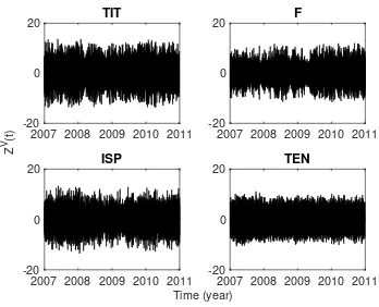
In Figures 1 and 2 are shown the trading volume and the logarithmic change of the trading volume for the 4 stocks in the analyzed period.
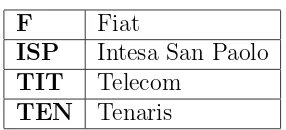
F Fiat
ISP Intesa San Paolo
TIT Telecom
TEN Tenaris
Table 1: Stocks used in the application and their symbols
2007 2008 2009 2010 20110 2
4 6 10
8 TIT
2007 2008 2009 2010 20110 2
4 6 10
7 F
2007 2008 2009 2010 20110 2
4 10
8 ISP
2007 2008 2009 2010 2011 Time (year)
0 5 10
Volume 106 TEN
2007 2008 2009 2010 2011 -20
0 20
TIT
2007 2008 2009 2010 2011 -20
0 20
F
2007 2008 2009 2010 2011 -20
0 20
ISP
2007 2008 2009 2010 2011 Time (year)
-20 0 20
Z
V (t)
TEN
TIT
1 2 3 4 5
0 1 2 3 10
5 F
1 2 3 4 5
0 2 4 10
5
ISP
1 2 3 4 5
0 1 2 3 10
5 TEN
1 2 3 4 5
States 0 1 2 3
Number of Occupancy
105
{−∞,−4,−1,1,4,∞}. The number of times that ZV(t) fall in each state is shown in Figure 3.
Following D’Amico & Petroni (2012b) we use as definition of the function
fλ in (4) an exponentially weighted moving average (EWMA) of the squares of ZV(t) which has the following expression:
fλ(Jn−1−k, Tn, a) =
and consequently the index process becomes
InV(λ) =
n(λ) was also discretized into 5 states of low, medium low, medium, medium high and high volume variation. Using these definitions and discretizations we estimated, for each stock, the probabilities defined in the previous section by using their estimators directly from real data. By means of Monte Carlo simulations we were able to produce, for each of the 4 stocks, a synthetic time series.
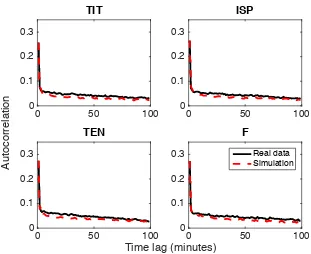
Each time series is a realization of the stochastic process described in the previous section with the same time length as real data. Statistical features of these synthetic time series are then compared with the statistical features of real data. In particular, we tested our model for the ability to reproduce the autocorrelation functions of the absolute value of ZV(t) and the first passage time distribution.
We estimated Σ(τ) (see equation 5) for real data and for synthetic data and show in Figure 4 a comparison between them for all stocks. For each stock we estimated the percentage root mean square error (RMSE) the results are reported in Table 2.
It is possible to note that our model is able to reproduce almost perfectly the autocorrelation of the absolute value of the logarithmic volume change stocks.
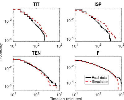
For each of the stocks in our database we estimate the first passage time distribution directly from the data (real data) and from the synthetic time series generated as described above.
0 50 100 0
0.1 0.2 0.3
TIT
0 50 100
0 0.1 0.2 0.3
ISP
0 50 100
0 0.1 0.2 0.3
TEN
0 50 100
Time lag (minutes) 0 0.1 0.2 0.3
Autocorrelation
F
Real data Simulation
Figure 4: Autocorrelation functions of the absolute value of ZV(t) for real data (solid line) and synthetic (dashed line) time series.
Stock Error F 3.6%
ISP 3.2%
TIT 3.0%
TEN 3.9%
101 102 103 10-4
10-2
TIT
101 102 103
10-4 10-2
ISP
101 102 103
10-4 10-2
TEN
101 102 103
Time lag (minutes) 10-4 10-2
Probability
F
Real data Simulation
Figure 5: First passage time distribution for ρ= 1000
5
Conclusions
In this paper we advanced the use of Weigthed-Indexed Semi-Markov Chain models for modeling high frequency financial volumes. We applied the model on real financial data and we shown that the model is able to reproduce important statistical fact of financial volumes as the autocorrelation function of the absolute values of volumes and the first passage time distribution. Further developments will be a more extensive application to other financial stocks and indexes and the proposal of a complete model where returns, volumes and durations are jointly described.
References
[1] C.T. Brownlees, F. Cipollini, G.M. Gallo. Journal of Financial Econo-metrics 9(3) (2011) 489-518.
[2] G. D’Amico, F. Petroni, ”A semi-Markov model with memory for price changes”, Journal of Statistical Mechanics: Theory and Experiment, P12009 (2011).
[4] G. D’Amico, F. Petroni, ”A semi-Markov model for price returns”, Phys-ica A 391 (2012) 4867-4876.
[5] G. D’Amico, F. Petroni, ”Multivariate high-frequency financial data via semi-Markov processes”, Markov Processes and Related Fields, 20 (2014) 415-434.
[6] G. D’Amico, F. Petroni, ”Copula Based Multivariate Semi-Markov Mod-els with Applications in High-Frequency Finance”, Submitted.
[7] F. De Jong, B. Rindi, ”The Microstructure of Financial Markets”, Cam-bridge University Press (2009), CamCam-bridge, New York.
[8] Jain, P., Joh, G., 1988. ”The dependence between hourly prices and trading volume”, Journal of Financial and Quantitative Analysis 23, 269-283.
[9] F. Mainardi, M. Raberto, R. Gorenflo, E. Scalas. Physica A 287 (2000) 468.
[10] S. Manganelli, ”Duration, Volume and Volatility impact of trades”, Journal of Financial Markets, 8, (2005) 377-399.
[11] B. Podobnik, D. Horvatic, A.M. Petersen, H.E. Stanley, ”Cross-Correlations between Volume Change and price Change”, PNAS, De-cember 29(52) (2009) 22079-22084.