Multimodal Freight Distribution & Economic
Development due to International Capacity Expansion
Jaehoon Kim1, Michael Anderson1,*, MD Sarder2, Chad Miller2,3
1Civil & Environmental Engineering, University of Alabama in Huntsville, Huntsville, USA 2Industrial Engineering Technology, University of Southern Mississippi, Long Beach, USA 3Department of Economic Development and Tourism, University of Southern Mississippi, Hattiesburg, USA
Abstract
This paper examines how international expansion may redistribute trade volumes across the intermodal system, including ports, waterways, railroads, and highways within the US Midwest and Southeast regions. The research includes a capacity analysis of existing transportation infrastructures to identify the possibility of capacity expansion. It also conducts economic development analysis to quantify the anticipated economic growth due to the increased freight movement in the potential sites. While developing the scenario based distribution model, this research focuses on the top six Asian countries that contribute 62 percent of current container imports. It also focuses on the top ten US ports, three more ports in the US that are critical to the study regions (Midwest and Southeast), and one Canadian port which is also critical to the Midwest and Southeast. Overall, there appears to be only minor economic impact on the Southeast and port states from the Panama Canal and the Port of Prince Rupert expansions. However, the Chicago-North area and other interior states experience significant impacts from the Panama Canal and the Port of Prince Rupert expansions under all three scenarios. This research provides decision makers with the information necessary to identify bottlenecks in the transportation network due to international capacity expansion and to identify/invest in targeted multimodal system improvements.Keywords
Panama Canal, International Freight, Network Modeling1. Introduction
The trade volume between the U.S. and Northeast Asia has continuously increased. The average freight volume growth rate from 2003 to 2012 is more than 4 percent; nevertheless the trade volume temporarily fell off due to the recent economic recession. Only five countries in Northeast Asia: China, Japan, South Korea, Taiwan and Hong Kong, handle roughly 53 percent of total container shipments to the U.S. [1]. Also, the U.S imports approximately 59 percent of containers from those five countries, and the volume has been consistently increasing. Due to the increasing freight volume from Northeast Asia, the Panama Canal Authority (PCA) [2] and the Port of Prince Rupert planned expansion projects, and the construction is underway. The Panama Canal expansion is expected to be finished in 2016, and the new canal will start to operate in 2016 [3]. The Port of Prince Rupert will initiate its operation in 2020.
There are three major routes for trade between Northeast Asia and East of the Mississippi regions: 1) using West coast ports and the U.S intermodal system for overland routes, 2) using East/Gulf coast ports via the Panama Canal, and 3)
* Corresponding author:
[email protected] (Michael Anderson) Published online at http://journal.sapub.org/ijtte
Copyright © 2015 Scientific & Academic Publishing. All Rights Reserved
using all water routes via the Suez Canal. Most recent information about shipping market share for routing from the Panama Canal Authority (PCA) shows that 61 percent of the trade volume from Asia to East Mississippi regions used the US intermodal system, and 38 percent of the freight was imported via the Panama Canal. The remaining 1 percent went through the Suez Canal [2].
affected by the expansion projects. During this step, generally accepted network databases were evaluated including: Highway Performance Monitoring System (HPMS), National Highway Planning Network (NHPN), and Freight Analysis Framework (FAF). Through this task, the most appropriate database was selected. The selected network was improved and used in the assignment step with the various scenarios. Lastly, the assignments of freight volume by truck and railroad are performed using the network database developed in the previous step. The zone system is appropriately adjusted on the network database and Origin-Destination trip tables (O/D tables) developed by UIC are adapted for the assignments.
This research also includes economic development analysis to quantify the economic impact expected from the increased freight movement and handling. The economic development analysis quantifies the economic growth due to the modeled change in freight movement and handling. Specifically, this part of the study converts the expected change in freight tonnage (thousand metric tons of containers) per region from the transportation model component into measures of economic competitiveness. It is forecast that there will be minor economic impact on Memphis-South and Port States regions from the Panama Canal and the Prince Rupert port expansions. This research finds that some port states will have to adjust their source ports for imports, but the impact on the overall regional economies will be insignificant. However, Chicago-North and other states regions will have significant impacts from the Panama Canal and the Port of Prince Rupert expansions under all three scenarios. Based on the economic development models, this research finds that many areas will experience limited development opportunities while some other areas will see significant increases in freight traffic and are prime targets for intermodal development. The cities likely to benefit include Fargo, ND; Joplin, MO; Meridian, MS; Bellevue, NE; St. Cloud, MI; Farragut, TN; Goodlettsville, TN; Prattville, AL; East Ridge, TN; Effingham, IL; and Hattiesburg, MS. These communities are expected to see significant increases in freight volume so are potential locations for intermodal facility development. The following sections discuss freight distribution scenario analysis, transportation infrastructure database development, network modeling and economic modeling.
2. Literature Review
For the analysis of route selection and optimization, active research and results have been discussed recently. Leachman [5] concluded that the container vessels calling on the West Coast ports are very sensitive to congestion and willing to change the destination port to less congested location. However, once congestion is relieved with infrastructure improvements and lead time is secured, San Pedro Bay is expected to remain its vessel calls from Asia. Levine et al. [6] estimated origin-destination matrix of US import
container freight with a linear program using a gravity model based on Transportation Analysis Zones (TAZ) which unit zone is larger than Bureau of Economic Analysis (BEA) unit area. Shintani et al. [7] used a genetic algorithm-based heuristic to solve the Knapsack problem in terms of calling sequences at ports.
Lei Fan et al. [8] constructed an optimization model considering vessel size, container shipper route, port, and shipping corridor, and concluded that Prince Rupert is a competitive alternative route for shipments to the Midwest Region while the Panama Canal’s expansion were identified with little impact of container flow.
Jula and Leachman [9] estimated the effects of container fees at the San Pedro Bay ports with Analytical model for Long- and Short-run supply chain model. They also introduced a queuing model to estimate container flow time considering volume, infrastructure, staffing level, and operating schedule focusing on Asian shipments coming into the U.S. rail intermodal terminals through the West Coast ports [10].
DeVuyst et al. [11] evaluated congestion with delay cost functions with a spatial optimization model for grain shipments on the Mississippi River. Lei Fan et al. [12] developed intermodal flow network model to analyze logistic system congestion since most ports observed congestion and capacity expansion is assumed to reduce congestion cost and waiting time. Most recently, Steven and Corsi [13] analyzed port attractiveness for containerized shipments from individual shipment data, port characteristics, and actual freight charges and concluded that larger shippers are more interested in factors affecting delivery speed than charges.
However, little research has analyzed import container freight with optimal route and attributes affecting route choices to the Midwest Region.
3. Freight Distribution Scenario
Analysis
The purpose of this step is to briefly introduce and to adapt the estimated container cargo distribution by UIC for this research. The research from UIC is used to analyze the imported container flow from seven Asian countries: China, Japan, Korea, Taiwan, Hong Kong, Mongolia and Macao to continental US regions [4]. The goal of this analysis is to estimate the container cargo distribution from seven Asian countries to the U.S. ports, and from the ports to the forty-eight states in the U.S. (in this research, Alaska and Hawaii are excluded).
data to FAF3 data, mode choice ratio was computed. FAF3 data is based on the Commodity Flow Survey results and it is regarded as proper information for mode choice. The study also collected 13 major international trade ports` capacities, as well as the expected Panama Canal capacity and the Prince Rupert port capacity after the expansion. Lastly, the cost information of ocean, rail, and truck transit for optimization process was gathered.
Based on the data, the containerized cargo flow optimization was performed and the Origin-Destination distributions (O/D distribution) which satisfied minimum shipping cost were estimated. The estimated O/D distributions consist of freight volume of all of the commodities from seven Asia countries to U.S. continental regions via thirteen U.S. international ports. Total three scenarios were prepared. The first scenario is the base scenario considering current capacity conditions without any expansion projects in 2012. The Panama Canal expansion will be finished in 2015, so the second scenario considers the increased capacity of the Panama Canal in 2019. The third scenario was developed by considering the expected capacity of the Prince Rupert Port Authority in Canada in 2020. The estimated O/D distributions indicate total freight flow from major U.S international ports to the states of US. In other words, each cell of the table indicates the imported cargo flow from each port to each state.
4. Transportation Infrastructure
Database Development
The network database is the one of the most important elements in transportation demand modelling, and the network represents flow of people or goods between origins and destinations [14]. In particular, a network database covering the US is required in this project are necessary, as well as various attributes such as link speed, capacity, number of lanes, and traffic counts.
Therefore, the task collects reliable network databases provided by reputable agencies, and evaluates the suitability of the databases. Then, the most appropriate database is selected through this task. The selected network is developed for this research. The developed network is used in the assignment step with various scenarios.
4.1. Highway Network Database Preparation
Network development represents the flow of people or goods between origins and destinations [15]. There are three principal types of network databases covering the US territory: Highway Performance Monitoring System (HPMS) [16], National Highway Planning Network (NHPN) [17], and Freight Analysis Framework (FAF3) [18].
The three network databases are compared to determine which is best suited for the project (see Table 1). All the databases are provided by Federal Highway Administration (FHWA) as GIS shapefiles. They also cover the whole US. Therefore, other attributes are considered to choose the
proper network for assignment process. Generally, links have various characteristics with the key characteristics being the network assignment process and/or network analysis, length of link, link cost, and link capacity [14]. Also, since it is not practical to collect traffic counts on the whole roadway system, Annual Average Daily Traffic (AADT) information is necessary to perform this project. Additionally, only the interstate network is considered as a major subject in this research.
HPMS and NHPN contain numbers of through lanes that can be used to calculate link capacity. FAF3 networks include computed capacity instead of number of through lanes. HPMS and NHPN have 2011 AADT but FAF3 has 2007 AADT and calibrated truck volume. All of the databases contain functional class of the network. Travel time is one of the most important factors to affect travel tendency. The travel time depends on vehicle speed, therefore, it can be computed by using the assigned speed [14]. FAF3 attributes contain computed speed but HPMS and NHPN do not have speed information. Though their links are categorized in each state by Federal Information Processing Standards (FIPS) and state FIPS codes are available in an attribute field. So, it is possible to add speed provided by Governors Highway Safety Association [19] on each link using the state’s FIPS codes.
The NHPN was chosen as best network database for this project and the necessary steps for preparation involved adding the speed to each roadway using ArcGIS.
Table 1. Comparing Characteristics of the Databases
HPMS NHPN FAF3
Provider FHWA FHWA FHWA
Format GIS shapefile GIS shapefile GIS shapefile
Coverage Whole U.S. Whole U.S. Whole U.S.
4.2. Railroad Network Preparation
The railroad network provided by nationatlas.gov was used in this research. The network contained polylines and attributes, but basic information such as speed and link length we added using ArcGIS. The network database consists of all of the railroads such as linehaul and Amtrak. We focus on linehaul railroad, especially, Class I railroads. The Class I railroad network was extracted from the shapefile. According to the Class I railroad statistics, classification are as follows:
− BNSF Railway (BNSF)
− Grand Trunk Corporation
− Kansas City Southern Railway (KCS)
− Norfolk Southern Combined Railroad Subsidiaries (NS)
− Soo Line Corporation
− Union Pacific Railroad (UP) [19]
Grand Trunk Corporation and Soo Line Corporation are not added on indices in the database. According to the article on the website of nationalatlas.gov, Grand Trunk Corporation consists of U.S operations of Canadian National (CN) [20]. Also, Soo Line is wholly owned subsidiary of Canadian Pacific (CP) [20]. So the Class I railroads are classified as BNSF, CSX, KCS, NS, CN, CP, and UP.
5. Transportation Network Impact
Modeling
The assignment of freight volume by truck and railroad uses the networks developed and origin/destination trip tables. In this task, FAF3 zone system is adopted and international ports are added as additional zones for the assignment. Also, the O/D tables are modified to meet FAF3 zone system and divided into truck O/D table and railroad O/D table. Using the network, zone system, and O/D tables, the freight assignment task is conducted in this task.
5.1. Construction of the Zone System
FAF3 consists of a total of 123 CFS regions and 8 international trade zones. This project focuses on the continental US so 120 zones out of 123 zones except Alaska and Hawaii are applied. Apart from the FAF3 zones, an additional 13 zones are added to represent international trade ports. These 13 international ports signed the Memorandum of Understanding to increase capacity The O/D matrix prepared in the previous chapter consists of 13 additional zones representing international trade ports for origin and 48 states excluding Alaska and Hawaii. The District of Columbia is considered as a zone. Therefore, the 13 international trade ports are represented as origins and 49 states are represented as destinations divided into 120 FAF3 zones.
5.2. Origin/Destination Table
The first step is to prepare a proper Origin/Destination matrix (O/D matrix) for freight assignment. The estimated O/D distributions, which are conducted by UIC, provide freight flows from thirteen international ports to forty-nine states in the US mainland as the destination zones. The O/D distributions mentioned before, consists of total freight tonnage by all modes between origin and destination. So, it is necessary to divide the total freight O/D distribution to freight by each mode O/D matrix. Also, we assume that all of the freight from the Port of Prince Rupert, Canada would use railway only. Each mode O/D matrix is rebuilt by using the mode ratio matrix (see Table 4 and 5).
The next step is to divide zone system of the state level
into the FAF3 zone system. Firstly, we assume two conditions to rebuild O/D matrix. The first condition is that each zone in the same state attracts same proportion of freight volume. The second condition is that each zone in the same state attracts different proportion of freight volume depending on the population. We build the new O/D matrices on these assumptions.
Secondly, the total freight volume in the each state is evenly divided by number of FAF3 zones in the each state in accordance with the first assumption. The reason why freight volumes are divided by the number of FAF3 zones is that it is necessary to compare between various scenarios. In the next step, we will rebuild O/D matrices under the second assumption based on the other criteria. For example, the freight volume in 2019 from the Los Angeles/Long Beach seaport (LA/LB) to Alabama by truck, for example, is 138,626 tons. Also, Alabama consists of three zones, Birmingham AL, Mobile AL, and remainder of Alabama. In this case, each freight volume from LA/LB port to each destination is 46,208.67 tons which is the result of total volume divided by 3. In this way, the first case O/D matrix is adjusted from original O/D pairs.
Lastly, each state`s volume is divided by population proportion. Generally, employment is the most frequently used variable to calculate consumed commodities by industries, and population is the most frequently used variable to estimate consumer goods. Therefore, population was selected as the main variable to rebuild the zone system because the distribution of population and employment are not significantly different due to FAF3 zone system, which is comprised of large size zones. The United States consists of a total of 3,143 counties including the District of Columbia. The county level of population data is collected from US Census data [21]. Then the counties are aggregated from FAF3 zones. After the aggregation, total population is calculated by state and by FAF3 zone. For example (see Table 2), the total freight flow from LA/LB port to Illinois by truck is 1,449,318.6 tons. Total population of Illinois is 12,830,632 where population of Zone 171 (Chicago area) is 8,700,058, population of Zone 172 (St. Louis area) is 703,664, and population of Zone 179 (remainder of Illinois) is 3,426,910. By using these values, each proportion for each state is computed. Finally, the freight volume to each zone is split into the proportions.
Table 2. Example of Adjusting O/D Matrix
O/D Illinois
LA/LB 1,449,318.6
Total Zone 171 Zone 172 Zone 179
Illinois
population 12,830,632 8,700,058 703,664 3,426,910
Proportion 100% 67.8% 5.5% 26.7%
Freight
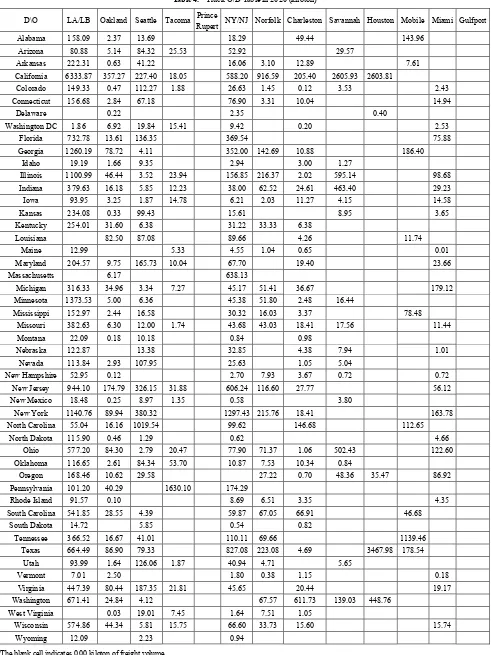
Table 4. Truck O/D Table in 2020 (kiloton)
D\O LA/LB Oakland Seattle Tacoma Prince
Rupert NY/NJ Norfolk Charleston Savannah Houston Mobile Miami Gulfport
Alabama 158.09 2.37 13.69 18.29 49.44 143.96
Arizona 80.88 5.14 84.32 25.53 52.92 29.57
Arkansas 222.31 0.63 41.22 16.06 3.10 12.89 7.61
California 6333.87 357.27 227.40 18.05 588.20 916.59 205.40 2605.93 2603.81
Colorado 149.33 0.47 112.27 1.88 26.63 1.45 0.12 3.53 2.43
Connecticut 156.68 2.84 67.18 76.90 3.31 10.04 14.94
Delaware 0.22 2.35 0.40
Washington DC 1.86 6.92 19.84 15.41 9.42 0.20 2.53
Florida 732.78 13.61 136.35 369.54 75.88
Georgia 1260.19 78.72 4.11 352.00 142.69 10.88 186.40
Idaho 19.19 1.66 9.35 2.94 3.00 1.27
Illinois 1100.99 46.44 3.52 23.94 156.85 216.37 2.02 595.14 98.68
Indiana 379.63 16.18 5.85 12.23 38.00 62.52 24.61 463.40 29.23
Iowa 93.95 3.25 1.87 14.78 6.21 2.03 11.27 4.15 14.58
Kansas 234.08 0.33 99.43 15.61 8.95 3.65
Kentucky 254.01 31.60 6.38 31.22 33.33 6.38
Louisiana 82.50 87.08 89.66 4.26 11.74
Maine 12.99 5.33 4.55 1.04 0.65 0.01
Maryland 204.57 9.75 165.73 10.04 67.70 19.40 23.66
Massachusetts 6.17 638.13
Michigan 316.33 34.96 3.34 7.27 45.17 51.41 36.67 179.12
Minnesota 1373.53 5.00 6.36 45.38 51.80 2.48 16.44
Mississippi 152.97 2.44 16.58 30.32 16.03 3.37 78.48
Missouri 382.63 6.30 12.00 1.74 43.68 43.03 18.41 17.56 11.44
Montana 22.09 0.18 10.18 0.84 0.98
Nebraska 122.87 13.38 32.85 4.38 7.94 1.01
Nevada 113.84 2.93 107.95 25.63 1.05 5.04
New Hampshire 52.95 0.12 2.70 7.93 3.67 0.72 0.72
New Jersey 944.10 174.79 326.15 31.88 606.24 116.60 27.77 56.12
New Mexico 18.48 0.25 8.97 1.35 0.58 3.80
New York 1140.76 89.94 380.32 1297.43 215.76 18.41 163.78
North Carolina 55.04 16.16 1019.54 99.62 146.68 112.65
North Dakota 115.90 0.46 1.29 0.62 4.66
Ohio 577.20 84.30 2.79 20.47 77.90 71.37 1.06 502.43 122.60
Oklahoma 116.65 2.61 84.34 53.70 10.87 7.53 10.34 0.84
Oregon 168.46 10.62 29.58 27.22 0.70 48.36 35.47 86.92
Pennsylvania 101.20 40.29 1630.10 174.29
Rhode Island 91.57 0.10 8.69 6.51 3.35 4.35
South Carolina 541.85 28.55 4.39 59.87 67.05 66.91 46.68
South Dakota 14.72 5.85 0.54 0.82
Tennessee 366.52 16.67 41.01 110.11 69.66 1139.46
Texas 664.49 86.90 79.33 827.08 223.08 4.69 3467.98 178.54
Utah 93.99 1.64 126.06 1.87 40.94 4.71 5.65
Vermont 7.01 2.50 1.80 0.38 1.15 0.18
Virginia 447.39 80.44 187.35 21.81 45.65 20.44 19.17
Washington 671.41 24.84 4.12 67.57 611.73 139.03 448.76
West Virginia 0.03 19.01 7.45 1.64 7.51 1.05
Wisconsin 574.86 44.34 5.81 15.75 66.60 33.73 15.60 15.74
Wyoming 12.09 2.23 0.94
Table 5. Railroad O/D Table in 2020 (kilotons)
D\O LA/LB Oakland Seattle Tacoma Prince
Rupert NY/NJ Norfolk Charleston Savannah Houston Mobile Miami Gulfport
Alabama 1.48 6.44 728.44 2.78 0.20
Arizona 2.48 0.04 7.18 20.19 0.20
Arkansas 3.95 0.51 21.09 0.04 8.58 4.72
California 19.55 8.25 12.16 13.44 563.99 15.47 0.13 23.26 370.38 857.48
Colorado 1.23 0.02 8.41 0.35 163.75 7.13
Connecticut 0.02 0.02 0.87
Delaware 1.48
Washington DC
Florida 2.40 0.03 108.12 0.14 0.35
Georgia 30.58 662.82 0.02 0.48 0.42 0.37
Idaho 0.01 0.01 1.34
Illinois 84.36 18.17 0.21 425.15 1.83 0.12 0.02 36.11
Indiana 8.18 0.29 56.13 0.46 0.11 39.66
Iowa 1.03
Kansas 0.35 1.21 46.63 1.49
Kentucky 0.18 0.85
Louisiana 0.71 1.09 1.42
Maine 0.01
Maryland 2.02 0.26 0.26 0.01
Massachusetts 0.13
Michigan 8.43 0.03 0.59 265.56 0.23 8.21 0.47 20.32
Minnesota 163.80 0.16 20.48 0.11 35.12
Mississippi 0.18 5.26 0.82 0.02
Missouri 7.06 0.18 10.89 0.45
Montana 0.02 0.12
Nebraska 10.73
Nevada 3.94 4.35 0.01
New Hampshire 0.06 0.25
New Jersey 54.36 14.76 1.13 742.71 10.42 6.04 17.69
New Mexico 0.05 1.89
New York 75.61 0.19 0.43 74.50 0.45 0.02 3.18 23.35
North Carolina 4.75 17.79 0.06 0.09 10.87 111.62
North Dakota 0.27
Ohio 13.31 2.16 0.20 222.95 0.01 52.89 0.12
Oklahoma 0.59 0.45
Oregon 24.25 0.21 74.09 2.11 137.24
Pennsylvania 1.09 0.26 1.22
Rhode Island 2.58
South Carolina 2.08
South Dakota 0.04
Tennessee 6.02 0.85 0.04
Texas 71.05 1.60 12.70 1050.59 32.47 0.64 0.02 278.55 159.63
Utah 0.10 0.01 0.92 4.52
Vermont
Virginia 10.43 48.71 0.11 1.22 12.16
Washington 7.81 0.01 0.04 56.32 0.52
West Virginia 0.04 0.28
Wisconsin 7.33 0.02 0.24 7.85 0.11
Wyoming 0.61
5.3. Scenario Preparation
We prepare O/D matrices for three years by using two different proportions. With these matrices, this study also classifies the research regions. This study specifically focuses on Midwest and Southeast as study regions. Therefore, the research regions are considered as two categories. The study categorizes all FAF3 zones and Midwest and U.S South regions for the assignment model. As a result of these processes a total of twelve scenarios are prepared for freight volume by truck assignment (see Table 3).
5.4. Assignment of Truck Freight Flows
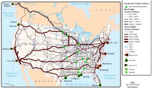
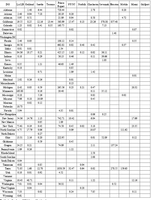
For assignment, single matrix equilibrium using time methodology is used. Firstly, link travel time is calculated and added to each link. Speed limit data and link distance were prepared in the previous step. Using the databases link travel time is calculated by CUBE/Voyager. Then, based on the prepared network, the freight volume by truck is assigned using the computed link travel time. Example output of the freight assignments are illustrated as Figures 1 and 2. As mentioned above, the expected O/D distributions were estimated as volume of all of the commodities. The O/D distributions can be converted if each commodity would be estimated by using conversion factors. However, the available source is total commodity volume, thus the freight
volume is assigned on the network. It has limitations of the network calibration and validation because of the object of the network assignment. Therefore, the network calibration and validation work are not performed in this study.
Table 3. Assignment Scenarios
Scenario Year Research subject regions
Proportion of State Freight Volume
1 2012
All FAF3 zones
State Volume / Numbers of FAF3 Zones in the State
2 2019
3 2020
4 2012
Midwest and U.S South
Regions
State Volume / Numbers of FAF3 Zones in the State
5 2019
6 2020
7 2012
All FAF3 zones
State Volume / Population Proportion
8 2019
9 2020
10 2012
Midwest
And U.S South Regions
State Volume / Population Proportion
11 2019
12 2020
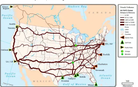
Figure 2. Result of Scenario 11: Truck Assignment (2019)
5.5. Assignment of Railroad Freight Flow
For the railroad assignment step zone connectors are set up so that distance is zero with some assumptions. There are two major routes connecting the Port of Prince Rupert, Canada and the United States. One is the route via the Washington state border and the other route is via the North Dakota border. We assume that there is no freight flow from Prince Rupert to east of Mississippi river regions via Seattle or Washington state. Also, it is expected that freight volume from the port of Prince Rupert would tend to use Canadian National railway service.
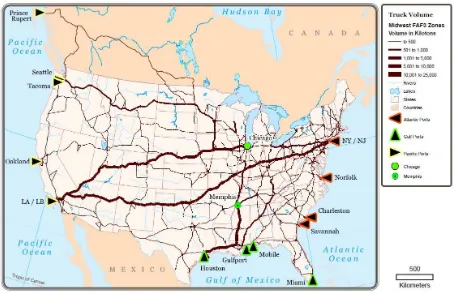
A total of twelve scenarios are prepared for the assignment step. The scenarios are built using the same methodologies as freight O/D matrix by truck. Also, the assignment method is the same as the truck mode analysis. In other words, the assignment uses travel time as a main factor to calculate equilibrium model. According to the Federal Railroad Administration, the operating speed limits vary with railroad conditions. However, most of railway conditions are not opened as public information. Therefore, assumption is made that the speed limit of the railroad network is sixty mile per hour. The output of the freight assignments are illustrated is Figure 3 and 4.
5.6. Model Strengths and Limitations
One of the key aspects of this research was to develop “Optimized Freight Distribution” Model. This model identified the routes, modes, and amount of freight
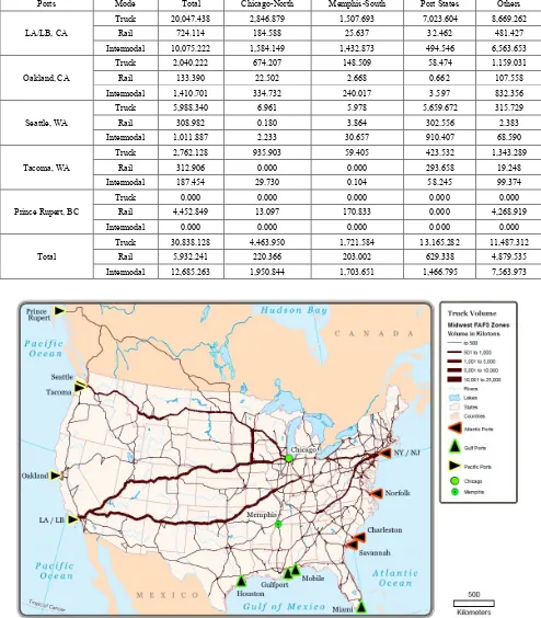
movements from 14 ports to primarily two markets (Memphis & South and Chicago & North). This distribution is ideal and minimizes the cost of freight distribution. For example, following table shows the optimum distribution of containers from selected West coast ports to two markets (Memphis & South and Chicago & North), port states and other states. In reality, shipping companies may choose to ship via different modes and different amounts based on their business models and hence pay more to do that.
Figure 3. Results of Scenario 8: Railroad Assignment (2019)
Table 6. Estimated Container Freight Mode Choice from the West Coast Ports to the U.S. in 2019 (after the Panama Canal Expansion) based on optimized model
Ports Mode Total Chicago-North Memphis-South Port States Others
LA/LB, CA
Truck 20,047.438 2,846.879 1,507.693 7,023.604 8,669.262
Rail 724.114 184.588 25.637 32.462 481.427
Intermodal 10,075.222 1,584.149 1,432.873 494.546 6,563.653
Oakland, CA
Truck 2,040.222 674.207 148.509 58.474 1,159.031
Rail 133.390 22.502 2.668 0.662 107.558
Intermodal 1,410.701 334.732 240.017 3.597 832.356
Seattle, WA
Truck 5,988.340 6.961 5.978 5,659.672 315.729
Rail 308.982 0.180 3.864 302.556 2.383
Intermodal 1,011.887 2.233 30.657 910.407 68.590
Tacoma, WA
Truck 2,762.128 935.903 59.405 423.532 1,343.289
Rail 312.906 0.000 0.000 293.658 19.248
Intermodal 187.454 29.730 0.104 58.245 99.374
Prince Rupert, BC
Truck 0.000 0.000 0.000 0.000 0.000
Rail 4,452.849 13.097 170.833 0.000 4,268.919
Intermodal 0.000 0.000 0.000 0.000 0.000
Total
Truck 30,838.128 4,463.950 1,721.584 13,165.282 11,487.312
Rail 5,932.241 220.366 203.002 629.338 4,879.535
Intermodal 12,685.263 1,950.844 1,703.651 1,466.795 7,563.973
Figure 6. Result of Scenario 11: Truck Assignment (2019), Midwest Freight Analysis Framework 3 [FAF3] Zones with Proportion of State Freight Volume by Population Proportion in each State. Modeling after Panama Canal expansion, but before Prince Rupert expansion
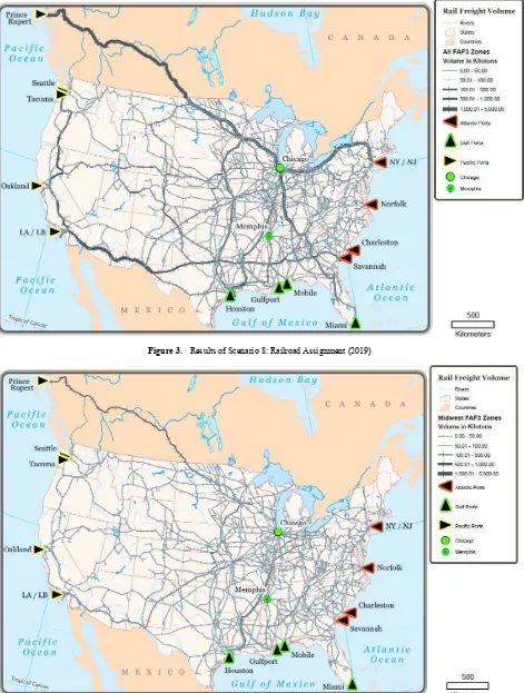
Figure 7. Result of Scenario 12: Truck Assignment (2020), Midwest Freight Analysis Framework 3 [FAF3] Zones with Proportion of State Freight Volume by Population Proportion in each State. Modeling after Panama Canal expansion and Prince Rupert expansion
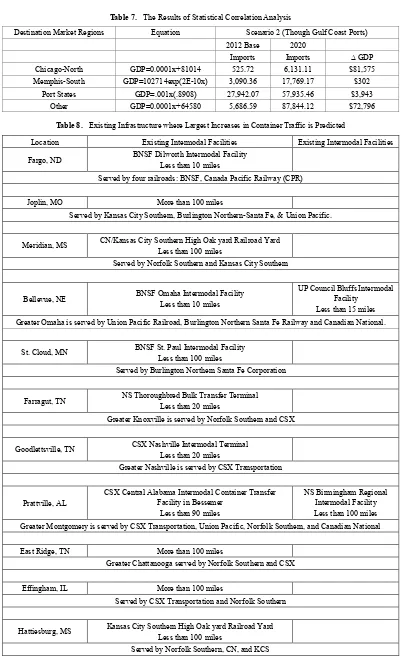
6. Economic Development Analysis
Based on the models, potential communities for freight based-economic development were determined and expected regional competitiveness impacts projected. The 11 cities in Table 7 are expected to see the largest increase in traffic and
volume. Rail volume was rated with a higher value than truck due to inability to move tracks. The GIS model was adapted from the 12 truck and 12 rail scenarios.
Site specific factors of the 11 potential intermodal development locations need to be considered. Table 7 provides the cities which are potential locations for intermodal facility development because they are expected to see significant increases in freight volume along with details of existing container intermodal transfer facilities near the identified cities along with major rail lines. According to a 2011 Transportation Research Board’s report (Steele et al. 2011), the primary criteria for intermodal facility location selection are as follows 1) access to markets or customers, 2) availability of transportation networks, 3) availability of workforce, 4) total cost of operation, 5) proximity to ports 6) permitting and regulations, and 7) availability and cost of ability space. These factors will need to be considered at each location to see if increased capacity is warranted based on increased freight volume.
6.1. Economic Development Analysis Methodology for Regional Competiveness
The second study objective of the economic development analysis in this study is to convert the expected change in freight tonnage (thousand metric tons of containers) per state from the Panama Canal expansion into measures of economic competitiveness (i.e., Gross Domestic Product by state). Gross Domestic Product (GDP), formerly Gross
State Product, by state is the state counterpart of the Nation's gross domestic product. GDP is calculated as the sum of what consumers, businesses, and government spend on final goods and services, plus investment and net foreign trade. The GDP by state estimates are used widely in both the public and private sectors. It is commonly used in econometric modelling and by state and local economic development offices.
In order to model the projected impact of change in import tonnage on GDP by region, the historical statistical relationship of import tonnage to GDP by state in the region was determined. For containerized import tonnage by state, the WISERTrade database was used. WISERTrade only has the confidence to release the state import data from 2008 so only five years of data was used for the analysis (The containerized data is available in the Port HS from 2003 and District HS database from 2002). State GDP was taken from the U.S. Department of Commerce Bureau of Economic Analysis for 2008 to 2012.
A statistical correlation analysis was conducted for all fifty states by the University of Southern Alabama. The fit of the statistical model varied greatly from a R2 of 0.05 for Illinois to 0.93 for Alaska. The fit at the regional level used in this analysis was much better. The ranges were from 0.94 for the Chicago-North region to 0.83 for the port regions. Because of the large variation at the state level, only the regional analysis is presented.
Table 7. The Results of Statistical Correlation Analysis
Destination Market Regions Equation Scenario 2 (Though Gulf Coast Ports)
2012 Base 2020
Imports Imports ∆ GDP
Chicago-North GDP=0.0001x+81014 525.72 6,131.11 $81,575
Memphis-South GDP=102714exp(2E-10x) 3,090.36 17,769.17 $302
Port States GDP=.001x(.8908) 27,942.07 57,935.46 $3,943
Other GDP=0.0001x+64580 5,686.59 87,844.12 $72,796
Table 8. Existing Infrastructure where Largest Increases in Container Traffic is Predicted
Location Existing Intermodal Facilities Existing Intermodal Facilities
Fargo, ND BNSF Dilworth Intermodal Facility
Less than 10 miles
Served by four railroads: BNSF, Canada Pacific Railway (CPR)
Joplin, MO More than 100 miles
Served by Kansas City Southern, Burlington Northern-Santa Fe, & Union Pacific.
Meridian, MS CN/Kansas City Southern High Oak yard Railroad Yard Less than 100 miles
Served by Norfolk Southern and Kansas City Southern
Bellevue, NE BNSF Omaha Intermodal Facility
Less than 10 miles
UP Council Bluffs Intermodal Facility
Less than 15 miles
Greater Omaha is served by Union Pacific Railroad, Burlington Northern Santa Fe Railway and Canadian National.
St. Cloud, MN BNSF St. Paul Intermodal Facility
Less than 100 miles
Served by Burlington Northern Santa Fe Corporation
Farragut, TN NS Thoroughbred Bulk Transfer Terminal
Less than 20 miles
Greater Knoxville is served by Norfolk Southern and CSX
Goodlettsville, TN CSX Nashville Intermodal Terminal Less than 20 miles
Greater Nashville is served by CSX Transportation
Prattville, AL
CSX Central Alabama Intermodal Container Transfer Facility in Bessemer
Less than 90 miles
NS Birmingham Regional Intermodal Facility Less than 100 miles
Greater Montgomery is served by CSX Transportation, Union Pacific, Norfolk Southern, and Canadian National
East Ridge, TN More than 100 miles
Greater Chattanooga served by Norfolk Southern and CSX
Effingham, IL More than 100 miles
Served by CSX Transportation and Norfolk Southern
Hattiesburg, MS Kansas City Southern High Oak yard Railroad Yard Less than 100 miles
6.2. Statistical Correlation Analysis Findings
Several scenario analysis were run and consistently the Chicago-North region was most impacted. Table 8 presents a typical scenario and X represents freight in kilograms. This scenario modeled the impact of the expansions to the Panama Canal and the Port of Prince Rupert on imports through the Gulf Ports. Under this scenario, all the regions will experience an increase in tonnage of imports. The impact on regional economies of this increase in imports is more pronounced for Chicago-North and Other states regions. This same pattern was found in all the scenarios run.
7. Conclusions
This research contributes to freight assignment as it describes the estimation of freight flow at the FAF3 zones using various scenarios. The FAF3 zone system and additional 13 international ports are built for the assignment task. The O/D tables are also modified to meet the developed zone system. As a result of the task, Figures 1 through 4 show the results of the assignments for freight flow with regard to the expansion projects. Large amount of freight volume from Asia is forecast to be diverted from ports on the West Coast to East and Gulf Coast in 2019 after the Panama Canal expansion. In addition, the freight volume directly arriving in the US is expected to be diffused to Prince Rupert after its port expansion in 2020.
It is also expected that there will be little economic impact on Memphis-South and Port States regions. On the other hand, Chicago-North and other states regions will have significant impacts from the Panama Canal and the Prince Rupert expansions. Based on economic development models, the study finds eleven cities which are potential locations for the expansion of intermodal facilities.
As mentioned above, this research focuses on the freight assignment of volumes of tons rather than number of trucks or railway carriages. Assignment of truck trips or rail trips can be performed using trip O/D tables that can be converted from the volume O/D tables by using the conversion factors provided by FHWA. However, the estimated O/D table in this research consists of total volume of all of commodity flow instead of each commodity flow. The traffic counts for further research are added in this network database. If each commodity flow O/D table would be estimated, the assignment of trips can be performed, as well as analysis of congestion or bottleneck due to the expansion project can be accomplished.
ACKNOWLEDGEMENTS
The authors would like to thank the Center for Freight Infrastructure Research and Education (CFIRE) for funding the research.
REFERENCES
[1] U.S. Department of Transportation, "Maritime Administration Office of Statistical & Economical Analysis," [Online]. Available: http://www.marad.dot.gov/library_landi ng_page/data_and_statistics/Data_and_Statistics.htm#Trade %20Statistics. [Accessed 17 April 2014].
[2] P. C. Authority, "Proposal for the Expansion of the Panama Canal: Third Set of Locks Project," Autoridad Del Canal De Panama, 2006.
[3] U.S. Department of Transportation, "Panama Canal Expansion Study, Phase I Report: Development in Trade and National and Global Economics," U.S. Department of Transportation, 2013.
[4] S. Ko, B. Karimi and A. Mohammadian, "Scenario Analysis of Containerized Freight Distribution into the Midwest Region in Response to Capacity Expansions," in Transportation Research Board, Washington D.C., 2014. [5] R. C. Leachman, "Port and modal allocation of waterborne
containerized imports from Asia to the United States," Transportation Research Part E: Logistics and Transportation Review, vol. 44, no. 2, pp. 313-331, 2008.
[6] B. Levine, L. Nozick and D. Jones, "Estimating an origina-destination table for US imports of waterborne containerized freight," Transportation Research Part E: Logistics and Transportation Review, vol. 45, no. 4, pp. 611-626, 2009.
[7] K. Shintani, A. Imai, E. Nishimura and S. Papadimitriou, "The container shipping network design problem with empty container repositioning," Transportation Research Part E: Logistics and Transportation Review, vol. 43, no. 1, pp. 39-59, 2007.
[8] L. Fan, W. W. Wilson and D. Tolliver, "Optimal network flows for containerized imports to the United States," Transportation Research Part E: Logistics and Transportation Review, vol. 46, no. 5, pp. 735-749, 2010.
[9] P. Jula and R. C. Leachman, "Long- and Short-Run supply-chain optimization models for the allocation and congestion management of containerized imports from Asia to the United States," Transportation Research Part E: Logistics and Transportation Review, vol. 47, no. 5, pp. 593-608, 2011.
[10] R. C. Leachman and P. Jula, "Estimating flow times for containerized imports from Asia to the United States through the Western rail network," Transportation Research Part E: Logistics and Transportation Review, vol. 48, no. 1, pp. 296-309, 2012.
[11] E. DeVuyst, W. W. Wilson and B. Dahl, "Longer-term forecasting and risks in spatial optimization models: The world grain trade," Transportation Research Part E: Logistics and Transportation Review, vol. 45, no. 3, pp. 472-485, 2009. [12] L. Fan, W. W. Wilson and B. Dahl, "Congestion, port expansion and spatial competition for US container imports," Transportation Research Part E: Logistics and Transportation Review, vol. 48, no. 6, pp. 1121-1136, 2012.
48, no. 4, pp. 881-895, 2012.
[14] M. Bell and Y. Ilda, Transportation Network Analysis, Wiley, 1997.
[15] D. M. Meyer and J. E. Miller, Urban Transportation Planning, McGraw-Hill, 2001.
[16] FHWA, "Highway Performance Monitoring System," [Online]. Available: http://www.fhwa.dot.gov/policyinforma tion/hpms.cfm. [Accessed 5 August 2013].
[17] FHWA, "Planning Process," [Online]. Available: http://www.fhwa.dot.gov/planning/processes/tools/nhpn/. [Accessed 4 September 2013].
[18] FHWA, "Freight Analysis Framework 3 User Guide," [Online]. Available: http://www.ops.fhwa.dot.gov/freight/fre
ight_analysis/faf/faf3/userguide/index.htm#s24. [Accessed 5 October 2013].
[19] G. H. S. Association, "Speed Limit Laws," [Online]. Available:http://www.ghsa.org/html/stateinfo/laws/speedlim it_laws.html. [Accessed 2013 10 September].
[20] AAR, "Class I Railroad Statistics," 10 May 2012. [Online]. Available:https://www.aar.org/StatisticsAndPublications/Do cuments/AAR-Stats-2012-05-10.pdf.
[21] nationalatlas.gov, "Overview of U.S. Freight Railroads," 5 August 2013. [Online]. Available: http://nationalatlas.gov/art icles/transportation/a_freightrr.html#four.
![Figure 6. Result of Scenario 11: Truck Assignment (2019), Midwest Freight Analysis Framework 3 [FAF3] Zones with Proportion of State Freight Volume by Population Proportion in each State](https://thumb-ap.123doks.com/thumbv2/123dok/3898690.1856260/11.595.92.513.77.348/scenario-assignment-analysis-framework-proportion-freight-population-proportion.webp)