Combinatorial Transforms : Applications in
Lossless Image Compression
E. Syahrul
1, J. Dubois
2, V. Vajnovszki
3LE2I - Universit´e de Bourgogne
B.P. 47 870, 21078 Dijon Cedex - France
{elfitrin.syahrul1, julien.dubois2, vvajnov3}@u-bourgogne.fr
Abstract
Common image compression standards are usually based on fre-quency transform such as Discrete Cosine Transform. We present a different approach for lossless image compression, which is based on a combinatorial transform. The main transform is Burrows Wheeler Transform (BWT) which tends to reorder symbols according to their following context. It becomes one of promising compression approach based on context modeling. BWT was initially applied for text com-pression software such as BZIP2; nevertheless it has been recently
ap-plied to the image compression field. Compression schemes based on the Burrows Wheeler Transform have been usually lossless; therefore we implement this algorithm in medical imaging in order to recon-struct every bit. Many variants of the three stages which form the original compression scheme can be found in the literature. We pro-pose an analysis of the latest methods and the impact of their associa-tion and present an alternative compression scheme with a significant improvement over the current standards such asJPEG and JPEG2000.
Keywords: BWT, Lossless (image) compression, combinatorial trans-form.
1
Introduction
presents the improvement and analysis of BWT methods particularly imple-mented for image compression. We analyze the effects of each stage of BWT pre- and post-processing. The results are compared withJPEGandJPEG2000.
2
Original method based on BWT
A typical Burrows Wheeler Transform method that has been proposed by Burrows and Wheeler for lossless text compression consists of 3 stages as seen in Figure 1 [7], where
• BWT is the Burrows Wheeler Transform itself that tends to group similar characters together,
• GST is the Global Structure Transform that transforms the output of BWT local structure redundancy to a global redundancy using a ranking list. It produces sequences of contiguous zeros,
• DC is a Data Coding.
Input data
BW T GST DC Output
...data
✲ ✲ ✲ ✲
Figure 1: Original scheme of BWT method.
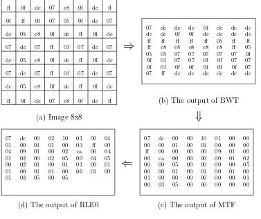
The stages are processed sequentially from left to right. The output of a stage becomes the input of the next stage. BWT as a main transform rearranges the input data using a sorting algorithm. The output content is exactly the same with the input, except the ordering. Figure 2 gives a simple example how BWT works in a small image. Pixels are encoded by a pair of hexadecimal values. The image is generated to assume that scanning the data left to right where there are not two identical consecutive symbols. BWT as a context based transform tends to group similar pixels together as seen in Figure 2(b). This transform does not reduce the data size; by contrast it adds a few bytes information as a primary index to decode the data. The detailed work of BWT and other related transforms will be explained below.
BWT
ff 0f dc 07 c8 0f dc ff 0f ff 0f 07 05 0f dc 07
07 dc dc dc 0f dc dc dc dc 05 c8 0f dc ff 0f dc dc dc 0f 0f dc dc dc dc ff ff ff ff ff 05 ff ff 07 dc 07 ff 0f 07 dc 07
⇒
ff c8 c8 c8 c8 c8 ff 0505 05 07 07 07 07 07 0f dc 05 c8 0f dc ff 0f dc 0f 0f 07 07 0f 0f 07 07 0f 0f 0f 0f 0f 0f 0f 07 07 dc 07 ff 0f 07 dc 07 07 ff dc dc dc dc dc dc dc 05 c8 0f dc ff 0f dc
ff 0f dc 07 c8 0f dc ff (b) The output of BWT
(a) Image 8x8
⇓
07 dc 00 02 10 01 00 04 07 dc 00 00 10 01 00 00 01 00 01 01 00 03 ff 00 00 00 01 00 01 00 00 00 04 09 01 00 02 ca 00 04 ff 00 00 00 00 09 01 00 01 02 00 02 05 00 04 05 00 ca 00 00 00 00 01 02 00 02 01 00 01 01 00 01
⇐
00 00 05 00 00 00 00 05 01 00 01 01 00 06 01 00 00 00 01 00 01 00 01 00 01 03 05 00 05 01 00 00 00 00 00 00 01. 00 03 05 00 00 00 00 00
(d) The output of RLE0 (c) The output of MTF
Figure 2: Example how BWCA works in a small image 8×8.
Rotated BWT input F L
1 ff 0fdc07c80fdc ff 0f ff 0f07050fdc07 13 05 0f dc 07 ff 0f dc07c8 0f dc ff 0f ff 0f07
2 0f dc07 c8 0f dc ff 0f ff 0f 0705 0f dc07 ff 12 07 05 0f dc 07 ff 0f dc07c8 0f dc ff 0f ff 0f
3 dc07 c8 0f dc ff 0f ff 0f 0705 0f dc07 ff 0f 4 07 c8 0f dc ff 0f ff 0f 0705 0f dc 07 ff 0fdc
4 07c8 0f dc ff 0f ff 0f 0705 0f dc 07 ff 0f dc 16 07 ff 0f dc 07c8 0f dc ff 0f ff 0f 0705 0fdc
5 c8 0f dc ff 0f ff 0f 0705 0f dc07 ff 0f dc 07 11 0f 0705 0f dc07 ff 0f dc07c8 0f dc ff 0f ff
6 0f dc ff 0f ff 0f 0705 0f dc07 ff 0f dc07 c8 2 0f dc07 c8 0f dc ff 0f ff 0f 0705 0f dc07ff
7 dc ff 0f ff 0f 0705 0f dc07 ff 0f dc07 c8 0f 14 0f dc07 ff 0f dc07 c8 0f dc ff 0f ff 0f 0705
8 ff 0f ff 0f 0705 0f dc07 ff 0f dc 07 c8 0f dc 6 0f dc ff 0f ff 0f 0705 0f dc07 ff 0f dc07c8
9 0f ff 0f 07 05 0f dc07 ff 0f dc07 c8 0f dc ff 9 0f ff 0f 07 05 0f dc07 ff 0f dc07 c8 0f dcff
10 ff 0f 07 05 0f dc07 ff 0f dc07 c8 0f dc ff 0f 5 c8 0f dc ff 0f ff 0f 0705 0f dc07 ff 0f dc07
11 0f 0705 0f dc07 ff 0f dc07c8 0f dc ff 0f ff 3 dc 07 c8 0f dc ff 0f ff 0f 0705 0f dc07 ff 0f
12 0705 0f dc 07 ff 0f dc07c8 0f dc ff 0f ff 0f 15 dc 07 ff 0f dc07 c8 0f dc ff 0f ff 0f 07050f
13 05 0f dc 07 ff 0f dc07c8 0f dc ff 0f ff 0f 07 7 dc ff 0f ff 0f 0705 0f dc07 ff 0f dc07 c80f
14 0f dc07 ff 0f dc07 c8 0f dc ff 0f ff 0f 07 05 10 ff 0f 07 05 0f dc07 ff 0f dc07 c8 0f dc ff 0f
15 dc07 ff 0f dc07 c8 0f dc ff 0f ff 0f 0705 0f 1 ff 0fdc07c80fdc ff 0f ff 0f07050fdc 07 ←15
16 07 ff 0f dc 07c8 0f dc ff 0f ff 0f 0705 0f dc 8 ff 0f ff 0f 0705 0f dc07 ff 0f dc 07 c8 0fdc (a) Rotated BWT input. (b) Sorted BWT rotations.
Position input context link 1 07 05 07
2 0f 07 01 3 dc 07 10 4 dc 07 15 5 ff 0f 02
6 ff 0f 11
7 05 0f 12 8 c8 0f 13 9 ff 0f 14 10 07 c8 08
11 0f dc 03
12 0f dc 04 13 0f dc 16 14 0f ff 05
→15 07 ff 06←
16 dc ff 09
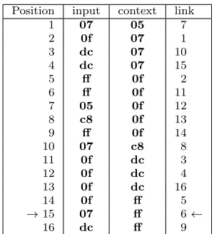
Figure 4: The BWT inverse transform.
represented in Figure 3(b). The position of original data is named primary index (equals to 15 in our example). This information is required for the reconstruction process. The last column (L) of this matrix and the primary index are the BWT output. As it can be seen in this example, BWT output tends to groups similar pixels together.
The reverse BWT [9] is principally just another permutation of the orig-inal data. Figure 4 shows how this process works. The second column of this figure is the BWT output of the data in Figure 3. The third column (called here context) is obtained from the second one by sorting its elements in ascending order. The link in the fourth column refers to the position of the context in the input (the second column). For repeated symbols the
ith occurrence of a context symbol corresponds to the ith occurrence of the same symbol in the data input. The process is started from position 15 (the primary index) where the first pixel value of the original data is placed. It refers to the contextf f (as the first pixel of original data) and also refers to link 6, as a clue of next position to the second element of original data. So, the next position is 6 which refers to 0f and gives the next link to the next output. Therefore each step gives the permuted pixel value as output and will process the whole file, because of the cyclic rotations.
GST
processes the input symbols sequentially. Every input of MTF is moved to the front of the list, so the input symbols that occur often are transformed into small indices. Runs of repeated symbols are transformed into zeros. Some authors proposed other GST transforms such as Move One From Front (M1FF), Move One From Front Two (M1FF2), Frequency Count (FC), etc. These transforms will be discussed in Section 6.
Data Coding
A data coding essentially based on Entropy Coding. Burrows and Wheeler propose to use Run Length Encoding Zeros (RLE0) after MTF since it pro-duces a lot of zeros, and then Huffman Coding or Arithmetic Coding to in-crease data compression [7]. Some approaches use Arithmetic Coding, which offers the best compression rates [11]. Further, Arithmetic Coding translates the entire data into numbers represented in certain base rather than trans-lating each data symbol into a series of digit in certain base. Therefore, AC approach is often more optimal than Huffman Coding.
Since the MTF output tends to produce a lot of small pixels value, Fen-wick proposes an adaptive Arithmetic Coding that follows the skew distri-bution of MTF output [9]. More details on this process will be discussed in Section 7.
3
Corpus
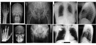
The BWT compression method has been applied for lossless text compression and do not take into account the data’s nature. Nevertheless, it can be applied successfully to image, as we will discuss in the next section. The lossless approach is obviously appropriate to medical image compression, which is expected to be lossless. Our experiments use 100 medical images selected from IRMA (Image Retrieval in Medical Applications) database [12] and Lukas Corpus [13]. The images are extracted randomly. IRMA database consists of primary and secondary digitized X-ray films in portable network graphics (PNG) and tagged image file format (TIFF), 8 bits per pixel (8 bpp),
examples of images are shown in Figure 5. The image sizes are between 101 KB and 4684 KB. And for the Lukas Corpus, we are using two dimensional 8 bit radiographs in TIFF format.
Figure 5: Example of tested images. From left to right: hand; head; pelvis; chest frontal and chest lateral.
ways to scan the images as a BWT pre-processing step.
4
Linearization Scheme
BWT method is used to compress two-dimensional images, but the input of BWT is a one dimensional sequence. Thus, the image has to be converted from two dimensional image into one dimensional sequence. This conversion is referred to as linearization or scan path. Some codings, as Arithmetic Coding or BWT itself, depend on the relative order of gray scale values, they are therefore sensitive to the linearization method used.
(a) Left (b) Left-Right (c) Up-Down (d) Spiral (e) Zigzag
Figure 6: Linearization methods.
Some of the popular linearization schemes are given in Figure 6. We have tested 8 such different methods; namely: scanning image from left to right (L), left to right then right to left (LR), up to down then down to up (UD), zigzag (ZZ), spiral, divide image into small blocks 8×8, small blocks 8×8 covering the image in zigzag, and small blocks 3×3 covering the image in zigzag.
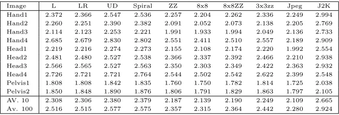
Table 1: Image compression ratios for different type of scan path.
Image L LR UD Spiral ZZ 8x8 8x8ZZ 3x3zz Jpeg J2K Hand1 2.372 2.366 2.547 2.536 2.257 2.204 2.262 2.336 2.249 2.994 Hand2 2.260 2.251 2.390 2.382 2.091 2.052 2.073 2.138 2.205 2.769 Hand3 2.114 2.123 2.253 2.221 1.991 1.933 1.994 2.049 2.136 2.733 Hand4 2.685 2.679 2.830 2.802 2.551 2.411 2.510 2.557 2.189 2.909 Head1 2.219 2.216 2.274 2.273 2.155 2.108 2.174 2.220 1.992 2.554 Head2 2.481 2.480 2.527 2.538 2.366 2.337 2.392 2.466 2.210 2.938 Head3 2.566 2.565 2.527 2.563 2.350 2.303 2.349 2.422 2.363 2.932 Head4 2.726 2.721 2.721 2.764 2.544 2.502 2.542 2.622 2.399 2.548 Pelvis1 1.808 1.808 1.842 1.835 1.760 1.750 1.782 1.814 1.725 2.038 Pelvis2 1.850 1.848 1.890 1.876 1.806 1.791 1.829 1.863 1.797 2.105 AV. 10 2.308 2.306 2.380 2.379 2.187 2.139 2.190 2.249 2.109 2.665 Av. 100 2.516 2.515 2.577 2.575 2.357 2.315 2.364 2.442 2.280 2.924
influences BWT methods performance. Image scan vertically (up-down) is slightly better than spiral method. Over the 100 images tested, 49 of them give the better result using up-down scan and 47 using spiral scan. The worst compression ratios are obtained using scan image in a block 8 ×8 (85 images), and zigzag mode (14 images). This preprocessing stage can increase the compression ratios around 4% than conventional scanning. In other words, the neighborhood of pixels influences the permutation yields by the BWT.
This result also shows that BWT method is better thanJPEGbut inferior
than JPEG2000. For all images tested, 91 give better CR than JPEG, and
among them 10 are better than JPEG2000. This preliminary result shows
that scanning the image up-down and in spiral improves compression ratios. Therefore our future tests will use spiral or up-down stage.
5
BWT and its improvement
BWT is based on a sorting algorithm. There are several methods to improve the performance of sorting process, but they do not influence BWT results. Burrows and Wheeler suggested suffix tree to improve sorting process [7]. Other authors suggest suffix array or their own sorting algorithm [14–16].
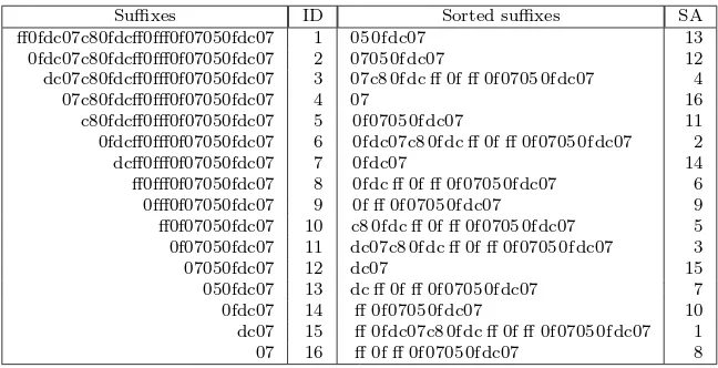
Figure 7 shows the relationship between BWT and suffix array for the same input given in Figure 3, and we consider the input data is Im, then n
is the length of Im, and so in this example n = 16.
Suffixes ID Sorted suffixes SA ff0fdc07c80fdcff0fff0f07050fdc07 1 05 0f dc07 13 0fdc07c80fdcff0fff0f07050fdc07 2 0705 0f dc07 12 dc07c80fdcff0fff0f07050fdc07 3 07c8 0f dc ff 0f ff 0f 0705 0f dc07 4 07c80fdcff0fff0f07050fdc07 4 07 16 c80fdcff0fff0f07050fdc07 5 0f 0705 0f dc07 11 0fdcff0fff0f07050fdc07 6 0f dc07c8 0f dc ff 0f ff 0f 0705 0f dc07 2 dcff0fff0f07050fdc07 7 0f dc07 14 ff0fff0f07050fdc07 8 0f dc ff 0f ff 0f 0705 0f dc07 6 0fff0f07050fdc07 9 0f ff 0f 0705 0f dc07 9 ff0f07050fdc07 10 c8 0f dc ff 0f ff 0f 0705 0f dc07 5 0f07050fdc07 11 dc07c8 0f dc ff 0f ff 0f 0705 0f dc07 3 07050fdc07 12 dc07 15 050fdc07 13 dc ff 0f ff 0f 0705 0f dc07 7 0fdc07 14 ff 0f 0705 0f dc07 10 dc07 15 ff 0f dc07c8 0f dc ff 0f ff 0f 0705 0f dc07 1 07 16 ff 0f ff 0f 0705 0f dc07 8
Figure 7: Relationship between BWT and suffix arrays (SA).
matrix of Figure 3(a) are ignored. For example the first line of Figure 3(b) was placed in line 13 of the rotated original data, so the rotations matrix for this line begins with the 13th symbol till the 16th symbol then followed by
the 1st till the 12th symbols to complete the sorted rotations matrix. If the
added symbols are omitted, this first line is equal to the first line of sorted suffixes (first line in the third column of Figure 7).
The BWT output can be computed using suffix array (SA) as:
L(i) =
½
Im[SA[i]−1], if SA[i]6= 1
Im[n], otherwise. (1)
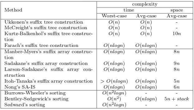
Hence, it does not need to create the sorted rotations matrix to obtain BWT output (Figure 3(a) and (b)). Nevertheless, finding suffix sorting algo-rithms that run in linear worst case time is still an open problem. Figure 8 shows a few different methods for BWT computation [17]. We use the BWT of Yuta Mori that is based on SA-IS algorithm to construct the BWT out-put [18]. It reduces processing time and decrease memory requirements.
6
GST and its modifications
Method
Farach’s suffix tree construction O(nlogn) O(nlogn) -Manber-Myers’s suffix array
construc-tion
O(nlogn) O(nlogn) 8n
Sadakane’s suffix array construction O(nlogn) O(nlogn) 9n
Larson-Sadakane’s suffix array con-struction
O(nlogn) O(nlogn) 8n
Itoh-Tanaka’s suffix array construction > O(nlogn) O(nlogn) 5n
Nong’s SA-IS O(nlogn) O(nlogn) 6n
Burrows-Wheeler’s sorting O(n2logn) -
-Bentley-Sedgewick’s sorting O(n2) O(nlogn) 5n+stack
Sedward’s sorting O(n2logn) -
-Figure 8: Different sorting algorithms used for BWT.
MTF maintains the list of all possible symbols (MTF list), which order is modified during the process. The list can be considered as a stack and is used to obtain the output. Each input value is coded with its rank in the list. This stack is then updated: the input value is pushed at the top of the list. Therefore, the rank of this input symbol becomes zero. Consequently, a run of N identical symbols is then coded with the symbol followed by N−1 zeros.
Most references show the efficiency of MTF, especially for text compres-sion. Table 2 and Table 3 in the 2nd and the 3rd column give the results
of BWT method for image compression without and with MTF. Here we can see that MTF part is significant. The compression ratios decrease for 6 images. Nevertheless, using scan image up-down, the average of compression ratios increase of approximately 3% for 10 images presented and 4% for the total database. And for scan image spiral, the compression ratio increases around 2% for 10 images and also 4% for total image database.
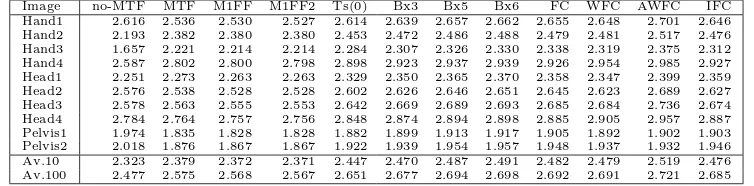
Table 2: The comparative results for MTF and its variants with up-down scan image.
Table 3: The comparative results for MTF and its variants with spiral scan image.
Image no-MTF MTF M1FF M1FF2 Ts(0) Bx3 Bx5 Bx6 FC WFC AWFC IFC Hand1 2.616 2.536 2.530 2.527 2.614 2.639 2.657 2.662 2.655 2.648 2.701 2.646 Hand2 2.193 2.382 2.380 2.380 2.453 2.472 2.486 2.488 2.479 2.481 2.517 2.476 Hand3 1.657 2.221 2.214 2.214 2.284 2.307 2.326 2.330 2.338 2.319 2.375 2.312 Hand4 2.587 2.802 2.800 2.798 2.898 2.923 2.937 2.939 2.926 2.954 2.985 2.927 Head1 2.251 2.273 2.263 2.263 2.329 2.350 2.365 2.370 2.358 2.347 2.399 2.359 Head2 2.576 2.538 2.528 2.528 2.602 2.626 2.646 2.651 2.645 2.623 2.689 2.627 Head3 2.578 2.563 2.555 2.553 2.642 2.669 2.689 2.693 2.685 2.684 2.736 2.674 Head4 2.784 2.764 2.757 2.756 2.848 2.874 2.894 2.898 2.885 2.905 2.957 2.887 Pelvis1 1.974 1.835 1.828 1.828 1.882 1.899 1.913 1.917 1.905 1.892 1.902 1.903 Pelvis2 2.018 1.876 1.867 1.867 1.922 1.939 1.954 1.957 1.948 1.937 1.932 1.946 Av.10 2.323 2.379 2.372 2.371 2.447 2.470 2.487 2.491 2.482 2.479 2.519 2.476 Av.100 2.477 2.575 2.568 2.567 2.651 2.677 2.694 2.698 2.692 2.691 2.721 2.685
Some authors change the MTF with other Global Structure Transform. We will test and analyze the impact of some of these transforms.
Balkenhol proposed the modification of MTF called Move One From Front (M1FF) [19]. This algorithm changes the work of the M1FF list. The in-put symbol from the second position in the M1FF list is moved to the first position; meanwhile the input from higher positions is moved to the second position. Furthermore, Balkenhol gives a modification of M1FF called Move One From Front Two (M1FF2). The symbol from the second position is moved to the first position of the M1FF2 list only when the previous trans-formed symbol was at the first position. Unfortunately, the results of our tests for these transforms decrease compression performance as seen in the column 4th and 5th of Table 2 and Table 3.
Albers also presented other list based algorithms, called Time Stamp (TS) [20]. The deterministic version of this algorithm is TimeStamp (0) or TS (0). While MTF use 256 symbols in its list, this transform uses a double length list. So the list contains 512 symbols and each symbol occurs twice. When the input data is processed, the position of an item is one plus the number of double symbols in front of that input symbol. Then the list is updated by moving the second symbol to the front. This method is also called “Best 2 of 3” algorithm based on the Chapin’s algorithm called a “Best
x of 2x−1” algorithm [21], because TS (0) uses 2×256 symbols in the list. Therefore, the list of a “Bestxof 2x−1” algorithm containsx×256 symbols. Here, we have tested a “Bestxof 2x−1” algorithm forx= 3, 5, and 6 (called
Bx3, Bx5 and Bx6, respectively for short) to see its impact in the BWT update methods (the original method with up-down or spiral image scan). The results of these transforms are shown in column 6th to 9th in the Table 2
and Table 3. The compression ratios using these transforms are better than those using MTF algorithm. The average compression performance increases till 9% for a “Bx6” algorithm using image scan up-down for the whole tested images.
quite different with the previous GST. There is a computation to count the symbols ranking. It gives the highest rank to the symbol with the highest frequency. This transform is not very effective since it takes time to favoring symbols [8]. The Weighted Frequency Count (WFC) improves FC transform by defining a function based on symbol frequencies [17]. It also counts the distance of symbols within a sliding window. The most frequent symbol has a higher weight. This approach does not give better compression ratios than FC in our tests. It can be seen in the column 10th and 11th of Table 2 and
Table 3. The improvement compression performance is obtained by a WFC modified called Advanced Weighted Frequency Count (AWFC). It counts a weight of symbol distribution. It is more complex than WFC, but it gives better compression ratios. These results can be seen in the column 12th of
Table 2 and Table 3.
Abel presents other GST method called Incremental Frequency Count (IFC) [11]. It is quite similar to WFC, but it is less complex and the CR is less than that obtained with WFC. The results of this transform can be seen in column 13th in the Table 2 and Table 3.
Table 2 and Table 3 show that AWFC is slightly better than a “Bx6”. But AWFC is more complex than a “Bx6” transform. It takes more time to count the distance of symbol. Therefore, for the next stage, we will use two of these transforms to analyze the Entropy Coding stage and to improve BWT method performances.
7
EC and its modifications
Burrows and Wheeler original paper uses RLE0 as the first step of EC, since there are a lot of zeros after MTF [7]. The function of RLE is to support the probability estimation of the next stage. A long run of zeros tends to overestimate the global symbol probability [19].
Our previous best results use AWFC or a “Bx6” algorithm for GST stage, Up-down or spiral image scan method for BWT pre-processing and a simple RLE0 followed by Arithmetic Coding for the EC stage. This compression scheme is referred as method M1 in 2nd and 3rd column of Table 4.
Lehmann et al. propose other RLE called Run Length Encoding two symbols (RLE2S) [4]. This coding separates the data stream and the runs so it does not interfere with the main data coding. It codes only two or more consecutive symbols into two symbols and the length of runs are placed in other data stream. This coding also decreases compression performance in our tests. The results of this second method (M2) are shown in the 6th and
Table 4: CR results for different EC methods.
M1 : M2 : M3 : M4 : M5 :
Image UD-BWT-GST UD-BWT- UD-BWT-GST UD-BWT- UD-BWT- JPEG
RLE0-AC RL2S-GST-AC modRLE-modAC GST-AC GST-modAC 2000
Bx6 AWFC Bx6 AWFC Bx6 AWFC Bx6 AWFC Bx6 AWFC Hand1 2.670 2.706 2.850 2.861 2.989 2.977 2.964 2.940 3.030 2.996 2.994 Hand2 2.477 2.513 2.591 2.600 2.733 2.710 2.640 2.611 2.759 2.709 2.776 Hand3 2.368 2.410 2.510 2.525 2.537 2.552 2.489 2.496 2.551 2.560 2.733 Hand4 2.945 3.000 3.108 3.120 3.289 3.280 3.173 3.156 3.329 3.297 2.909 Head1 2.367 2.400 2.483 2.480 2.512 2.505 2.502 2.490 2.520 2.506 2.554 Head2 2.637 2.672 2.786 2.793 2.833 2.834 2.827 2.816 2.848 2.836 2.937 Head3 2.654 2.695 2.828 2.837 2.921 2.922 2.900 2.890 2.952 2.940 2.932 Head4 2.843 2.902 3.046 3.058 3.206 3.187 3.164 3.128 3.254 3.202 2.673 Pelvis1 1.922 1.908 2.009 1.974 2.019 1.981 2.017 1.976 2.024 1.982 2.038 Pelvis2 1.969 1.950 2.069 2.027 2.075 2.030 2.081 2.034 2.081 2.032 2.105 Av.10 2.485 2.516 2.628 2.628 2.711 2.698 2.676 2.654 2.735 2.706 2.665 Av.100 2.699 2.724 2.860 2.849 2.955 2.930 2.931 2.890 2.987 2.939 2.924
Another RLE0 that never expands the file has been presented by Wheeler. This coding encodes the data as a binary value. Reference [9] discusses more details about this coding.
For the last coding, as stated above, Burrows and Wheeler suggest to use Arithmetic Coding. As mentioned by Abel in [11] that a specific Arith-metic Coder should be used, we cannot use a simple arithArith-metic coder with a common order-ncontext. GST stage increases the probability of lower input values (and so it decreases the probability of the higher values).
Therefore, Fenwick proposes an Arithmetic Coder with hierarchical cod-ing model for this skew distribution. We also tested this codcod-ing, referred as M3 in Table 5. The results of this method are presented in the 7th and 8th
column of Table 4. In contrast to the common methods related in literature, we propose to omit RLE stage on this compression scheme. Two chains are then proposed. They are respectively similar to the M1 and M3 schemes but do not include any RLE stage. Therefore, the first one uses a traditional AC and the second one, a modified AC.
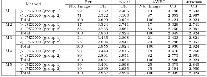
Table 5: CR results for different BWT methods.
Method Nb. ImageBx6 CR JPEG2000CR Nb. ImageAWFC CR JPEG2000CR M1 >JPEG2000(group 1) 29 3.132 2.486 13 3.196 2.633
<JPEG2000(group 2) 71 2.522 3.103 87 2.653 2.967 Total 100 2.699 2.924 100 2.724 2.924 M2 >JPEG2000(group 1) 17 3.324 2.741 17 3.329 2.741 <JPEG2000(group 2) 83 2.765 2.961 83 2.750 2.961 Total 100 2.860 2.924 100 2.849 2.924 M3 >JPEG2000(group 1) 24 3.435 2.868 21 3.433 2.821 <JPEG2000(group 2) 76 2.804 2.941 79 2.796 2.951 Total 100 2.955 2.924 100 2.930 2.924 M4 >JPEG2000(group 1) 20 3.449 2.815 18 3.416 2.768 <JPEG2000(group 2) 80 2.801 2.951 82 2.775 2.961 Total 100 2.931 2.924 100 2.890 2.924 M5 >JPEG2000(group 1) 30 3.401 2.898 25 3.375 2.845 <JPEG2000(group 2) 70 2.809 2.935 75 2.794 2.950 Total 100 2.987 2.924 100 2.939 2.924
analyze the results by splitting the image in two classes. The images which provide better compression ratios than JPEG2000 (>JPEG2000), referred as
group 1, and others (<JPEG2000), referred as group 2. This analysis is
pre-sented in Table 5. All the methods provide, for the group 1, a significant improvement of the average compression ratio over JPEG2000standard. The
method using a “Bx6” algorithm, provides a compression ratio improvement equals to 17% in comparison with JPEG2000. It is specially significant as it
concerns the higher number of images (30%). For the group 2, the modifi-cations on the BWT schemes (M2, M3, M4 and M5) enable the difference on the average CR between BWT method and JPEG2000 to be decreased.
As seen in Table 4, M5 using “Bx6” gives slightly better average CR than M4, and the lowest value of difference of average CR between BWT method and JPEG2000 for group 2. The same tendencies are observed for AWFC
methods.
8
Conclusion and Perspectives
We presented the state of the art of the application of BWT in lossless im-age compression. We analyzed the impact of each stim-age that has important role to improve compression performance. We also showed the BWT im-plementation in image is not similar to that in text. We should consider pre-processing, where this stage improves CR till 4%.
On the 100 medical images of the database, the average compression rate obtained with the proposed method is slightly better than with JPEG2000
standard. Nevertheless, this new approach based on combinatorial method provides much higher compression rate on some images. This fact has been observed on 30% of the tested images. For these images, the CR is in average 17% higher than theJPEG2000standard. Meanwhile, the other images (70%)
provide a CR which is only lower than 4%. These promising results offer two interesting perspectives. Firstly, we currently investigate the modification of EC stage to be more adapted with the BWT stage. A preliminary result shows that the merging of RLE and AC stage should be consider. Secondly, we consider developing an automatic image classification technique based on the image features (as the image texture) to split the images in two classes: those which provide the best results with the Burrows Wheeler compression scheme and those where the standard JPEG2000is more efficient. Therefore,
References
[1] M. Ciavarella and A. Moffat, “Lossless image compression using pixel reordering,” Proceedings of the twenty-seventh Australasian Computer Science Conference, pp. 125–132, 2004.
[2] N. R. Jalumuri, “A Study of Scanning Paths for BWT Based Image Compression,” Master’s thesis, 2004.
[3] X. Bai, J. S. Jin, and D. Feng, “Segmentation-based multilayer diagnosis lossless medical image compression,” inVIP ’05: Proceedings of the Pan-Sydney area workshop on Visual information processing, (Darlinghurst, Australia, Australia), pp. 9–14, Australian Computer Society, Inc., 2004.
[4] T. M. Lehmann, J., and C. Weis, “The impact of lossless image compres-sion to radiographs,” Proceeding. SPIE, vol. 6145, pp. 290–297, March 2006.
[5] Y. Wiseman, “Burrows-Wheeler based JPEG,” Data Science Journal, vol. 6, pp. 19–27, 2007.
[6] E. Syahrul, J. Dubois, V. Vajnovszki, T. Saidani, and M. Atri, “Loss-less image compression using Burrows Wheeler Transform (methods and techniques),” in SITIS ’08, pp. 338–343, 2008.
[7] M. Burrows and D. J. Wheeler, “A block-sorting lossless data compres-sion algorithm,” tech. rep., System Research Center (SRC) California, May 10, 1994.
[8] D. Adjeroh, T. Bell, and A. Mukherjee, The Burrows-Wheeler Trans-form: Data Compression, Suffix Arrays, and Pattern Matching . Springer US, june 2008.
[9] P. M. Fenwick, “Burrows–Wheeler compression: Principles and reflec-tions,” Theor. Comput. Sci., vol. 387, no. 3, pp. 200–219, 2007.
[10] J. L. Bentley, D. D. Sleator, R. E. Tarjan, and V. K. Wei, “A locally adaptive data compression scheme,” Commun. ACM, vol. 29, no. 4, pp. 320–330, 1986.
[12] T. M. Lehmann, M. O. G¨uld, C. Thies, B. Fischer, K. Spitzer, D. Key-sers, H. Ney, M. Kohnen, H. Schubert, and B. B. Wein, “Content-based image retrieval in medical applications,” 2004.
[13] “Lukas corpus.” http://www.data-compression.info/Corpora/LukasCorpus/index.htm.
[14] S. Kurtz and B. Balkenhol, “Space efficient linear time computation of the Burrows and Wheeler-Transformation,” incomplexity, Festschrift in honour of Rudolf Ahlswede’s 60th Birthday, pp. 375–384, 1999.
[15] G. Manzini, “Two space saving tricks for linear time lcp array compu-tation,” in Proc. SWAT. Volume 3111 of Lecture Notes in Computer Science, pp. 372–383, Springer, 2004.
[16] P. Ferragina, R. Giancarlo, G. Manzini, and M. Sciortino, “Boosting textual compression in optimal linear time,” ACM, vol. 52, pp. 688–713, July 2005.
[17] S. Deorowicz, Universal lossless data compression algorithms. PhD the-sis, Silesian University of Technology Faculty of Automatic Control, Electronics and Computer Science Institute of Computer Science, 2003.
[18] G. Nong, S. Zhang, and W. H. Chan, “Linear suffix array construction by almost pure induced-sorting,” Data Compression Conference, vol. 0, pp. 193–202, 2009.
[19] B. Balkenhol and Y. M. Shtarkov, “One attempt of a compression algo-rithm using the BWT.” SFB343: Discrete Structures in Mathematics, Preprint, Faculty of Mathematics, University of Bielefeld, 1999.
[20] S. Albers, “Improved randomized on-line algorithms for the list update problem,” SIAM J. Comput., vol. 27, no. 3, pp. 682–693, 1998.