Springer Texts in Statistics

(1)

Springer Texts in Statistics

Series Editors: G. Casella S. Fienberg I. Olkin

For further volumes:

(2)

(3)

Gareth James

• Daniela Witten

• Trevor Hastie

Robert Tibshirani

An Introduction to

Statistical Learning

with Applications in R

(4)

Operations

University of Southern California Los Angeles, CA, USA

Trevor Hastie

Department of Statistics Stanford University Stanford, CA, USA

Department of Biostatistics University of Washington Seattle, WA, USA

Robert Tibshirani Department of Statistics Stanford University Stanford, CA, USA

ISSN 1431-875X

ISBN 978-1-4614-7137-0 ISBN 978-1-4614-7138-7 (eBook) DOI 10.1007/978-1-4614-7138-7

Springer New York Heidelberg Dordrecht London

Library of Congress Control Number: 2013936251

printing 2017)

This work is subject to copyright. All rights are reserved by the Publisher, whether the whole or part of the material is concerned, specifically the rights of translation, reprinting, reuse of illustrations, recitation, broadcasting, reproduction on microfilms or in any other physical way, and transmission or information storage and retrieval, electronic adaptation, computer software, or by similar or dissim-ilar methodology now known or hereafter developed. Exempted from this legal reservation are brief excerpts in connection with reviews or scholarly analysis or material supplied specifically for the pur-pose of being entered and executed on a computer system, for exclusive use by the purchaser of the work. Duplication of this publication or parts thereof is permitted only under the provisions of the Copyright Law of the Publisher’s location, in its current version, and permission for use must always be obtained from Springer. Permissions for use may be obtained through RightsLink at the Copyright Clearance Center. Violations are liable to prosecution under the respective Copyright Law.

The use of general descriptive names, registered names, trademarks, service marks, etc. in this publi-cation does not imply, even in the absence of a specific statement, that such names are exempt from the relevant protective laws and regulations and therefore free for general use.

While the advice and information in this book are believed to be true and accurate at the date of publication, neither the authors nor the editors nor the publisher can accept any legal responsibility for any errors or omissions that may be made. The publisher makes no warranty, express or implied, with respect to the material contained herein.

Printed on acid-free paper

Springer is part of Springer Science+Business Media (www.springer.com)

Department of Data Sciences and

(5)

To our parents:

Alison and Michael James

Chiara Nappi and Edward Witten

Valerie and Patrick Hastie

Vera and Sami Tibshirani

and to our families:

Michael, Daniel, and Catherine

Tessa, Theo, and Ari

Samantha, Timothy, and Lynda

(6)

(7)

Preface

Statistical learning refers to a set of tools for modeling and understanding complex datasets. It is a recently developed area in statistics and blends with parallel developments in computer science and, in particular, machine learning. The field encompasses many methods such as the lasso and sparse regression, classification and regression trees, and boosting and support vector machines.

With the explosion of “Big Data” problems, statistical learning has be-come a very hot field in many scientific areas as well as marketing, finance, and other business disciplines. People with statistical learning skills are in high demand.

One of the first books in this area—The Elements of Statistical Learning (ESL) (Hastie, Tibshirani, and Friedman)—was published in 2001, with a second edition in 2009. ESL has become a popular text not only in statis-tics but also in related fields. One of the reasons for ESL’s popularity is its relatively accessible style. But ESL is intended for individuals with ad-vanced training in the mathematical sciences.An Introduction to Statistical Learning(ISL) arose from the perceived need for a broader and less tech-nical treatment of these topics. In this new book, we cover many of the same topics as ESL, but we concentrate more on the applications of the methods and less on the mathematical details. We have created labs illus-trating how to implement each of the statistical learning methods using the popular statistical software packageR. These labs provide the reader with valuable hands-on experience.

This book is appropriate for advanced undergraduates or master’s stu-dents in statistics or related quantitative fields or for individuals in other

(8)

disciplines who wish to use statistical learning tools to analyze their data. It can be used as a textbook for a course spanning one or two semesters.

We would like to thank several readers for valuable comments on prelim-inary drafts of this book: Pallavi Basu, Alexandra Chouldechova, Patrick Danaher, Will Fithian, Luella Fu, Sam Gross, Max Grazier G’Sell, Court-ney Paulson, Xinghao Qiao, Elisa Sheng, Noah Simon, Kean Ming Tan, and Xin Lu Tan.

It’s tough to make predictions, especially about the future.

-Yogi Berra

Los Angeles, USA Gareth James

Seattle, USA Daniela Witten

Palo Alto, USA Trevor Hastie

(9)

1 Introduction

An Overview of Statistical Learning

Statistical learningrefers to a vast set of tools forunderstanding data. These tools can be classified as supervised or unsupervised. Broadly speaking, supervised statistical learning involves building a statistical model for pre-dicting, or estimating, anoutputbased on one or moreinputs. Problems of this nature occur in fields as diverse as business, medicine, astrophysics, and public policy. With unsupervised statistical learning, there are inputs but no supervising output; nevertheless we can learn relationships and struc-ture from such data. To provide an illustration of some applications of statistical learning, we briefly discuss three real-world data sets that are considered in this book.

Wage Data

In this application (which we refer to as theWagedata set throughout this book), we examine a number of factors that relate to wages for a group of males from the Atlantic region of the United States. In particular, we wish to understand the association between an employee’sageandeducation, as well as the calendaryear, on hiswage. Consider, for example, the left-hand panel of Figure 1.1, which displayswageversusagefor each of the individu-als in the data set. There is evidence thatwageincreases withagebut then decreases again after approximately age 60. The blue line, which provides an estimate of the averagewage for a givenage, makes this trend clearer.

G. James et al.,An Introduction to Statistical Learning: with Applications in R, Springer Texts in Statistics, DOI 10.1007/978-1-4614-7138-7 1,

©Springer Science+Business Media New York 2013

(16)

Age

Wa

g

e

Year

Wa

g

e

20 40 60 80

50

100

200

300

50

100

200

300

50

100

200

300

2003 2006 2009 1 2 3 4 5

Education Level

Wa

g

e

FIGURE 1.1.Wage data, which contains income survey information for males

from the central Atlantic region of the United States.Left:wageas a function of

age. On average, wageincreases with ageuntil about 60years of age, at which

point it begins to decline. Center: wage as a function of year. There is a slow

but steady increase of approximately $10,000 in the average wage between 2003

and 2009. Right: Boxplots displaying wage as a function of education, with 1

indicating the lowest level (no high school diploma) and 5 the highest level (an

advanced graduate degree). On average,wageincreases with the level of education.

Given an employee’sage, we can use this curve topredicthiswage. However, it is also clear from Figure 1.1 that there is a significant amount of vari-ability associated with this average value, and so age alone is unlikely to provide an accurate prediction of a particular man’swage.

We also have information regarding each employee’s education level and theyearin which thewagewas earned. The center and right-hand panels of Figure 1.1, which displaywageas a function of bothyearandeducation, in-dicate that both of these factors are associated withwage. Wages increase by approximately $10,000, in a roughly linear (or straight-line) fashion, between 2003 and 2009, though this rise is very slight relative to the vari-ability in the data. Wages are also typically greater for individuals with higher education levels: men with the lowest education level (1) tend to have substantially lower wages than those with the highest education level (5). Clearly, the most accurate prediction of a given man’s wage will be obtained by combining hisage, hiseducation, and the year. In Chapter 3, we discuss linear regression, which can be used to predict wage from this data set. Ideally, we should predict wage in a way that accounts for the non-linear relationship between wage and age. In Chapter 7, we discuss a class of approaches for addressing this problem.

Stock Market Data

(17)

Yesterday

Today’s Direction

P

ercentage change in S&P

Two Days Previous

P

Down Up

Today’s Direction

Down Up

Today’s Direction

Down Up

−4

−2

0

2

4

6

−4

−2

0

2

4

6

−4

−2

0

2

4

6

Three Days Previous

P

FIGURE 1.2.Left:Boxplots of the previous day’s percentage change in the S&P

index for the days for which the market increased or decreased, obtained from the

Smarket data.Center and Right:Same as left panel, but the percentage changes for 2 and 3 days previous are shown.

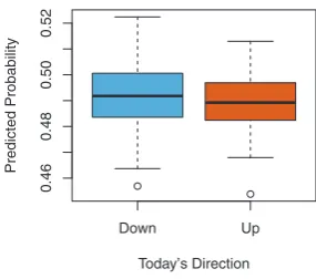
or qualitativeoutput. For example, in Chapter 4 we examine a stock mar-ket data set that contains the daily movements in the Standard & Poor’s 500 (S&P) stock index over a 5-year period between 2001 and 2005. We refer to this as the Smarketdata. The goal is to predict whether the index will increaseor decreaseon a given day using the past 5 days’ percentage changes in the index. Here the statistical learning problem does not in-volve predicting a numerical value. Instead it inin-volves predicting whether a given day’s stock market performance will fall into the Upbucket or the Downbucket. This is known as aclassification problem. A model that could accurately predict the direction in which the market will move would be very useful!

(18)

Down Up

0.46

0.48

0.50

0.52

Today’s Direction

Predicted Probability

FIGURE 1.3. We fit a quadratic discriminant analysis model to the subset

of the Smarket data corresponding to the 2001–2004 time period, and predicted

the probability of a stock market decrease using the 2005 data. On average, the predicted probability of decrease is higher for the days in which the market does decrease. Based on these results, we are able to correctly predict the direction of movement in the market 60% of the time.

Gene Expression Data

The previous two applications illustrate data sets with both input and output variables. However, another important class of problems involves situations in which we only observe input variables, with no corresponding output. For example, in a marketing setting, we might have demographic information for a number of current or potential customers. We may wish to understand which types of customers are similar to each other by grouping individuals according to their observed characteristics. This is known as a clusteringproblem. Unlike in the previous examples, here we are not trying to predict an output variable.

We devote Chapter 10 to a discussion of statistical learning methods for problems in which no natural output variable is available. We consider theNCI60 data set, which consists of 6,830 gene expression measurements for each of 64 cancer cell lines. Instead of predicting a particular output variable, we are interested in determining whether there are groups, or clusters, among the cell lines based on their gene expression measurements. This is a diﬃcult question to address, in part because there are thousands of gene expression measurements per cell line, making it hard to visualize the data.

(19)

−40 −20 0 20 40 60

−60

−40

−20

0

20

−60

−40

−20

0

20

Z1

−40 −20 0 20 40 60

Z1

Z2 Z2

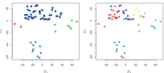
FIGURE 1.4. Left: Representation of the NCI60 gene expression data set in

a two-dimensional space, Z1 and Z2. Each point corresponds to one of the 64

cell lines. There appear to be four groups of cell lines, which we have represented

using diﬀerent colors.Right: Same as left panel except that we have represented

each of the14diﬀerent types of cancer using a diﬀerent colored symbol. Cell lines

corresponding to the same cancer type tend to be nearby in the two-dimensional space.

some loss of information, it is now possible to visually examine the data for evidence of clustering. Deciding on the number of clusters is often a diﬃ-cult problem. But the left-hand panel of Figure 1.4 suggests at least four groups of cell lines, which we have represented using separate colors. We can now examine the cell lines within each cluster for similarities in their types of cancer, in order to better understand the relationship between gene expression levels and cancer.

In this particular data set, it turns out that the cell lines correspond to 14 diﬀerent types of cancer. (However, this information was not used to create the left-hand panel of Figure 1.4.) The right-hand panel of Fig-ure 1.4 is identical to the left-hand panel, except that the 14 cancer types are shown using distinct colored symbols. There is clear evidence that cell lines with the same cancer type tend to be located near each other in this two-dimensional representation. In addition, even though the cancer infor-mation was not used to produce the left-hand panel, the clustering obtained does bear some resemblance to some of the actual cancer types observed in the right-hand panel. This provides some independent verification of the accuracy of our clustering analysis.

A Brief History of Statistical Learning

(20)

of least squares, which implemented the earliest form of what is now known aslinear regression. The approach was first successfully applied to problems in astronomy. Linear regression is used for predicting quantitative values, such as an individual’s salary. In order to predict qualitative values, such as whether a patient survives or dies, or whether the stock market increases or decreases, Fisher proposed linear discriminant analysis in 1936. In the 1940s, various authors put forth an alternative approach,logistic regression. In the early 1970s, Nelder and Wedderburn coined the term generalized linear modelsfor an entire class of statistical learning methods that include both linear and logistic regression as special cases.

By the end of the 1970s, many more techniques for learning from data were available. However, they were almost exclusivelylinearmethods, be-cause fittingnon-linearrelationships was computationally infeasible at the time. By the 1980s, computing technology had finally improved suﬃciently that non-linear methods were no longer computationally prohibitive. In mid 1980s Breiman, Friedman, Olshen and Stone introducedclassification and regression trees, and were among the first to demonstrate the power of a detailed practical implementation of a method, including cross-validation for model selection. Hastie and Tibshirani coined the termgeneralized addi-tive modelsin 1986 for a class of non-linear extensions to generalized linear models, and also provided a practical software implementation.

Since that time, inspired by the advent of machine learning and other disciplines, statistical learning has emerged as a new subfield in statistics, focused on supervised and unsupervised modeling and prediction. In recent years, progress in statistical learning has been marked by the increasing availability of powerful and relatively user-friendly software, such as the popular and freely available R system. This has the potential to continue the transformation of the field from a set of techniques used and developed by statisticians and computer scientists to an essential toolkit for a much broader community.

This Book

(21)

learning was starting to explode. ESL provided one of the first accessible and comprehensive introductions to the topic.

Since ESL was first published, the field of statistical learning has con-tinued to flourish. The field’s expansion has taken two forms. The most obvious growth has involved the development of new and improved statis-tical learning approaches aimed at answering a range of scientific questions across a number of fields. However, the field of statistical learning has also expanded its audience. In the 1990s, increases in computational power generated a surge of interest in the field from non-statisticians who were eager to use cutting-edge statistical tools to analyze their data. Unfortu-nately, the highly technical nature of these approaches meant that the user community remained primarily restricted to experts in statistics, computer science, and related fields with the training (and time) to understand and implement them.

In recent years, new and improved software packages have significantly eased the implementation burden for many statistical learning methods. At the same time, there has been growing recognition across a number of fields, from business to health care to genetics to the social sciences and beyond, that statistical learning is a powerful tool with important practical applications. As a result, the field has moved from one of primarily academic interest to a mainstream discipline, with an enormous potential audience. This trend will surely continue with the increasing availability of enormous quantities of data and the software to analyze it.

The purpose ofAn Introduction to Statistical Learning (ISL) is to facili-tate the transition of statistical learning from an academic to a mainstream field. ISL is not intended to replace ESL, which is a far more comprehen-sive text both in terms of the number of approaches considered and the depth to which they are explored. We consider ESL to be an important companion for professionals (with graduate degrees in statistics, machine learning, or related fields) who need to understand the technical details behind statistical learning approaches. However, the community of users of statistical learning techniques has expanded to include individuals with a wider range of interests and backgrounds. Therefore, we believe that there is now a place for a less technical and more accessible version of ESL.

(22)

in order to contribute to their chosen fields through the use of statistical learning tools.

ISLR is based on the following four premises.

1. Many statistical learning methods are relevant and useful in a wide range of academic and non-academic disciplines, beyond just the sta-tistical sciences.We believe that many contemporary statistical learn-ing procedures should, and will, become as widely available and used as is currently the case for classical methods such as linear regres-sion. As a result, rather than attempting to consider every possible approach (an impossible task), we have concentrated on presenting the methods that we believe are most widely applicable.

2. Statistical learning should not be viewed as a series of black boxes.No single approach will perform well in all possible applications. With-out understanding all of the cogs inside the box, or the interaction between those cogs, it is impossible to select the best box. Hence, we have attempted to carefully describe the model, intuition, assump-tions, and trade-oﬀs behind each of the methods that we consider.

3. While it is important to know what job is performed by each cog, it is not necessary to have the skills to construct the machine inside the box!Thus, we have minimized discussion of technical details related to fitting procedures and theoretical properties. We assume that the reader is comfortable with basic mathematical concepts, but we do not assume a graduate degree in the mathematical sciences. For in-stance, we have almost completely avoided the use of matrix algebra, and it is possible to understand the entire book without a detailed knowledge of matrices and vectors.

(23)

R years before they are implemented in commercial packages. How-ever, the labs in ISL are self-contained, and can be skipped if the reader wishes to use a diﬀerent software package or does not wish to apply the methods discussed to real-world problems.

Who Should Read This Book?

This book is intended for anyone who is interested in using modern statis-tical methods for modeling and prediction from data. This group includes scientists, engineers, data analysts, or quants, but also less technical indi-viduals with degrees in non-quantitative fields such as the social sciences or business. We expect that the reader will have had at least one elementary course in statistics. Background in linear regression is also useful, though not required, since we review the key concepts behind linear regression in Chapter 3. The mathematical level of this book is modest, and a detailed knowledge of matrix operations is not required. This book provides an in-troduction to the statistical programming language R. Previous exposure to a programming language, such as MATLAB or Python, is useful but not required.

We have successfully taught material at this level to master’s and PhD students in business, computer science, biology, earth sciences, psychology, and many other areas of the physical and social sciences. This book could also be appropriate for advanced undergraduates who have already taken a course on linear regression. In the context of a more mathematically rigorous course in which ESL serves as the primary textbook, ISL could be used as a supplementary text for teaching computational aspects of the various approaches.

Notation and Simple Matrix Algebra

Choosing notation for a textbook is always a diﬃcult task. For the most part we adopt the same notational conventions as ESL.

We will usento represent the number of distinct data points, or observa-tions, in our sample. We will letpdenote the number of variables that are available for use in making predictions. For example, theWagedata set con-sists of 12 variables for 3,000 people, so we haven= 3,000 observations and

p= 12 variables (such asyear,age, , and more). Note that throughout this book, we indicate variable names using colored font:Variable Name.

In some examples,pmight be quite large, such as on the order of thou-sands or even millions; this situation arises quite often, for example, in the analysis of modern biological data or web-based advertising data.

(24)

In general, we will letxij represent the value of thejth variable for the

ith observation, wherei= 1,2, . . . , n andj = 1,2, . . . , p. Throughout this book,iwill be used to index the samples or observations (from 1 ton) and

j will be used to index the variables (from 1 top). We letXdenote an_×p

For readers who are unfamiliar with matrices, it is useful to visualizeXas a spreadsheet of numbers withnrows andpcolumns.

At times we will be interested in the rows of X, which we write as

x1, x2, . . . , xn. Here xi is a vector of length p, containing the p variable measurements for the ith observation. That is,

xi=

(Vectors are by default represented as columns.) For example, for theWage data, xi is a vector of length 12, consisting of year, age, , and other values for the ith individual. At other times we will instead be interested in the columns ofX, which we write asx1,x2, . . . ,xp. Each is a vector of Using this notation, the matrixXcan be written as

(25)

TheT _{notation denotes the}_transpose_{of a matrix or vector. So, for example,}

We use yi to denote the ith observation of the variable on which we wish to make predictions, such as wage. Hence, we write the set of all n

observations in vector form as

y=

In this text, a vector of length n will always be denoted in lower case bold; e.g.

However, vectors that are not of lengthn(such as feature vectors of length

p, as in (1.1)) will be denoted inlower case normal font, e.g.a. Scalars will also be denoted inlower case normal font, e.g.a. In the rare cases in which these two uses for lower case normal font lead to ambiguity, we will clarify which use is intended. Matrices will be denoted using bold capitals, such as A. Random variables will be denoted usingcapital normal font, e.g.A, regardless of their dimensions.

Occasionally we will want to indicate the dimension of a particular ob-ject. To indicate that an object is a scalar, we will use the notationa_∈R. To indicate that it is a vector of length k, we will usea∈Rk _(or_a _∈_Rn

if it is of lengthn). We will indicate that an object is ar×smatrix using

A_∈Rr×s_.

(26)

of A and B is denotedAB. The (i, j)th element of AB is computed by multiplying each element of theith row ofAby the corresponding element of the jth column ofB. That is, (AB)ij =dk=1aikbkj. As an example, consider

A=

1 2 3 4

and B=

5 6 7 8

.

Then

AB=

1 2 3 4

5 6 7 8

=

1_×5 + 2_×7 1_×6 + 2_×8 3×5 + 4×7 3×6 + 4×8

=

19 22 43 50

.

Note that this operation produces an r_×smatrix. It is only possible to computeABif the number of columns ofAis the same as the number of rows ofB.

Organization of This Book

Chapter 2 introduces the basic terminology and concepts behind statisti-cal learning. This chapter also presents theK-nearest neighborclassifier, a very simple method that works surprisingly well on many problems. Chap-ters 3 and 4 cover classical linear methods for regression and classification. In particular, Chapter 3 reviews linear regression, the fundamental start-ing point for all regression methods. In Chapter 4 we discuss two of the most important classical classification methods,logistic regressionand lin-ear discriminant analysis.

A central problem in all statistical learning situations involves choosing the best method for a given application. Hence, in Chapter 5 we intro-ducecross-validationand thebootstrap, which can be used to estimate the accuracy of a number of diﬀerent methods in order to choose the best one. Much of the recent research in statistical learning has concentrated on non-linear methods. However, linear methods often have advantages over their non-linear competitors in terms of interpretability and sometimes also accuracy. Hence, in Chapter 6 we consider a host of linear methods, both classical and more modern, which oﬀer potential improvements over stan-dard linear regression. These include stepwise selection, ridge regression, principal components regression,partial least squares, and thelasso.

(27)

are discussed in Chapter 9. Finally, in Chapter 10, we consider a setting in which we have input variables but no output variable. In particular, we presentprincipal components analysis, K-means clustering, and hierarchi-cal clustering.

At the end of each chapter, we present one or more R lab sections in which we systematically work through applications of the various meth-ods discussed in that chapter. These labs demonstrate the strengths and weaknesses of the various approaches, and also provide a useful reference for the syntax required to implement the various methods. The reader may choose to work through the labs at his or her own pace, or the labs may be the focus of group sessions as part of a classroom environment. Within each R lab, we present the results that we obtained when we performed the lab at the time of writing this book. However, new versions of R are continuously released, and over time, the packages called in the labs will be updated. Therefore, in the future, it is possible that the results shown in the lab sections may no longer correspond precisely to the results obtained by the reader who performs the labs. As necessary, we will post updates to the labs on the book website.

We use the symbol to denote sections or exercises that contain more challenging concepts. These can be easily skipped by readers who do not wish to delve as deeply into the material, or who lack the mathematical background.

Data Sets Used in Labs and Exercises

In this textbook, we illustrate statistical learning methods using applica-tions from marketing, finance, biology, and other areas. TheISLR package available on the book website contains a number of data sets that are required in order to perform the labs and exercises associated with this book. One other data set is contained in the MASSlibrary, and yet another is part of the baseRdistribution. Table 1.1 contains a summary of the data sets required to perform the labs and exercises. A couple of these data sets are also available as text files on the book website, for use in Chapter 2.

Book Website

The website for this book is located at

(28)

Name Description

Auto Gas mileage, horsepower, and other information for cars.

Boston Housing values and other information about Boston suburbs.

Caravan Information about individuals oﬀered caravan insurance.

Carseats Information about car seat sales in 400 stores.

College Demographic characteristics, tuition, and more for USA colleges.

Default Customer default records for a credit card company.

Hitters Records and salaries for baseball players.

Khan Gene expression measurements for four cancer types.

NCI60 Gene expression measurements for 64 cancer cell lines.

OJ Sales information for Citrus Hill and Minute Maid orange juice.

Portfolio Past values of financial assets, for use in portfolio allocation.

Smarket Daily percentage returns for S&P 500 over a 5-year period.

USArrests Crime statistics per 100,000 residents in 50 states of USA.

Wage Income survey data for males in central Atlantic region of USA.

Weekly 1,089 weekly stock market returns for 21 years.

TABLE 1.1.A list of data sets needed to perform the labs and exercises in this

textbook. All data sets are available in the ISLR library, with the exception of

Boston (part ofMASS) andUSArrests(part of the base Rdistribution).

It contains a number of resources, including theRpackage associated with this book, and some additional data sets.

Acknowledgements

(29)

2 Statistical Learning

2.1 What Is Statistical Learning?

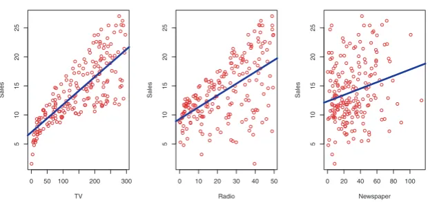
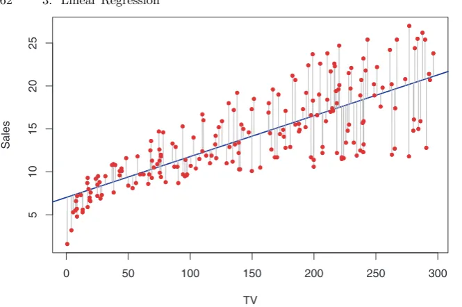
In order to motivate our study of statistical learning, we begin with a simple example. Suppose that we are statistical consultants hired by a client to provide advice on how to improve sales of a particular product. The Advertising data set consists of thesalesof that product in 200 diﬀerent markets, along with advertising budgets for the product in each of those markets for three diﬀerent media:TV, radio, and newspaper. The data are displayed in Figure 2.1. It is not possible for our client to directly increase sales of the product. On the other hand, they can control the advertising expenditure in each of the three media. Therefore, if we determine that there is an association between advertising and sales, then we can instruct our client to adjust advertising budgets, thereby indirectly increasing sales. In other words, our goal is to develop an accurate model that can be used to predict sales on the basis of the three media budgets.

In this setting, the advertising budgets are input variables whilesales

input variable

is anoutput variable. The input variables are typically denoted using the

output variable

symbol X, with a subscript to distinguish them. So X1 might be the TV budget, X2 the radio budget, and X3 the newspaper budget. The inputs

go by diﬀerent names, such as predictors, independent variables, features, _predictor

independent variable feature

or sometimes just variables. The output variable—in this case, sales—is

variable

often called the response or dependent variable, and is typically denoted

response dependent variable

using the symbolY. Throughout this book, we will use all of these terms interchangeably.

G. James et al.,An Introduction to Statistical Learning: with Applications in R, Springer Texts in Statistics, DOI 10.1007/978-1-4614-7138-7 2,

©Springer Science+Business Media New York 2013

(30)

0 50 100 200 300

51

0

1

5

2

0

2

5

TV

Sales

0 10 20 30 40 50

51

0

1

5

2

0

2

5

Radio

Sales

0 20 40 60 80 100

51

0

1

5

2

0

2

5

Newspaper

Sales

FIGURE 2.1.TheAdvertisingdata set. The plot displayssales, in thousands

of units, as a function of TV, radio, and newspaper budgets, in thousands of

dollars, for 200diﬀerent markets. In each plot we show the simple least squares

fit ofsalesto that variable, as described in Chapter 3. In other words, each blue

line represents a simple model that can be used to predictsalesusingTV,radio,

andnewspaper, respectively.

More generally, suppose that we observe a quantitative responseY andp

diﬀerent predictors, X1, X2, . . . , Xp. We assume that there is some relationship between Y and X = (X1, X2, . . . , Xp), which can be written in the very general form

Y =f(X) +ǫ. (2.1)

Heref is some fixed but unknown function ofX1, . . . , Xp, andǫis a random

error term, which is independent ofX and has mean zero. In this formula- _{error term} tion,f represents thesystematicinformation thatX provides aboutY.

systematic

As another example, consider the left-hand panel of Figure 2.2, a plot of incomeversusyears of educationfor 30 individuals in theIncomedata set. The plot suggests that one might be able to predictincomeusingyears of education. However, the functionf that connects the input variable to the output variable is in general unknown. In this situation one must estimate

f based on the observed points. Since Income is a simulated data set,f is known and is shown by the blue curve in the right-hand panel of Figure 2.2. The vertical lines represent the error terms ǫ. We note that some of the 30 observations lie above the blue curve and some lie below it; overall, the errors have approximately mean zero.

(31)

10 12 14 16 18 20 22

20

30

40

50

60

70

80

Years of Education

Income

10 12 14 16 18 20 22

20

30

40

50

60

70

80

Years of Education

Income

FIGURE 2.2.The Income data set.Left: The red dots are the observed values

ofincome(in tens of thousands of dollars) andyears of educationfor30

indi-viduals.Right:The blue curve represents the true underlying relationship between

income andyears of education, which is generally unknown (but is known in this case because the data were simulated). The black lines represent the error associated with each observation. Note that some errors are positive (if an ob-servation lies above the blue curve) and some are negative (if an obob-servation lies below the curve). Overall, these errors have approximately mean zero.

In essence, statistical learning refers to a set of approaches for estimating

f. In this chapter we outline some of the key theoretical concepts that arise in estimatingf, as well as tools for evaluating the estimates obtained.

2.1.1 Why Estimate

f

?

There are two main reasons that we may wish to estimate f: prediction andinference. We discuss each in turn.

Prediction

In many situations, a set of inputs X are readily available, but the output

Y cannot be easily obtained. In this setting, since the error term averages to zero, we can predictY using

ˆ

Y = ˆf(X), (2.2)

(32)

Years of Education

Senior ity

Income

FIGURE 2.3.The plot displays incomeas a function of years of education

andseniority in the Incomedata set. The blue surface represents the true

un-derlying relationship between income andyears of education and seniority,

which is known since the data are simulated. The red dots indicate the observed

values of these quantities for30individuals.

As an example, suppose thatX1, . . . , Xpare characteristics of a patient’s blood sample that can be easily measured in a lab, and Y is a variable encoding the patient’s risk for a severe adverse reaction to a particular drug. It is natural to seek to predict Y using X, since we can then avoid giving the drug in question to patients who are at high risk of an adverse reaction—that is, patients for whom the estimate of Y is high.

The accuracy of ˆY as a prediction for Y depends on two quantities,

which we will call the reducible errorand theirreducible error. In general, _reducible

error irreducible error

ˆ

f will not be a perfect estimate forf, and this inaccuracy will introduce some error. This error isreducible because we can potentially improve the accuracy of ˆfby using the most appropriate statistical learning technique to estimatef. However, even if it were possible to form a perfect estimate for

f, so that our estimated response took the form ˆY =f(X), our prediction would still have some error in it! This is because Y is also a function of

ǫ, which, by definition, cannot be predicted usingX. Therefore, variability associated withǫalso aﬀects the accuracy of our predictions. This is known as the irreducible error, because no matter how well we estimate f, we cannot reduce the error introduced by ǫ.

(33)

manufacturing variation in the drug itself or the patient’s general feeling of well-being on that day.

Consider a given estimate ˆf and a set of predictorsX, which yields the prediction ˆY = ˆf(X). Assume for a moment that both ˆf and X are fixed. Then, it is easy to show that

E(Y ₋Yˆ)2 = E[f(X) +ǫ₋fˆ(X)]2 = [f(X)−fˆ(X)]2

Reducible

+ Var(ǫ)

Irreducible

, (2.3)

whereE(Y ₋Yˆ)2_{represents the average, or}_{expected value, of the squared}

expected value

diﬀerence between the predicted and actual value of Y, and Var(ǫ)

repre-sents thevarianceassociated with the error term ǫ. _variance The focus of this book is on techniques for estimatingf with the aim of

minimizing the reducible error. It is important to keep in mind that the irreducible error will always provide an upper bound on the accuracy of our prediction forY. This bound is almost always unknown in practice.

Inference

We are often interested in understanding the way that Y is aﬀected as

X1, . . . , Xp change. In this situation we wish to estimatef, but our goal is not necessarily to make predictions forY. We instead want to understand the relationship betweenX andY, or more specifically, to understand how

Y changes as a function ofX1, . . . , Xp. Now ˆf cannot be treated as a black box, because we need to know its exact form. In this setting, one may be interested in answering the following questions:

• Which predictors are associated with the response?It is often the case that only a small fraction of the available predictors are substantially associated withY. Identifying the fewimportantpredictors among a large set of possible variables can be extremely useful, depending on the application.

• What is the relationship between the response and each predictor? Some predictors may have a positive relationship withY, in the sense that increasing the predictor is associated with increasing values of

Y. Other predictors may have the opposite relationship. Depending on the complexity off, the relationship between the response and a given predictor may also depend on the values of the other predictors.

(34)

In this book, we will see a number of examples that fall into the prediction setting, the inference setting, or a combination of the two.

For instance, consider a company that is interested in conducting a direct-marketing campaign. The goal is to identify individuals who will respond positively to a mailing, based on observations of demographic vari-ables measured on each individual. In this case, the demographic varivari-ables serve as predictors, and response to the marketing campaign (either pos-itive or negative) serves as the outcome. The company is not interested in obtaining a deep understanding of the relationships between each in-dividual predictor and the response; instead, the company simply wants an accurate model to predict the response using the predictors. This is an example of modeling for prediction.

In contrast, consider theAdvertisingdata illustrated in Figure 2.1. One may be interested in answering questions such as:

– Which media contribute to sales?

– Which media generate the biggest boost in sales?or

– How much increase in sales is associated with a given increase in TV advertising?

This situation falls into the inference paradigm. Another example involves modeling the brand of a product that a customer might purchase based on variables such as price, store location, discount levels, competition price, and so forth. In this situation one might really be most interested in how each of the individual variables aﬀects the probability of purchase. For instance, what eﬀect will changing the price of a product have on sales? This is an example of modeling for inference.

Finally, some modeling could be conducted both for prediction and infer-ence. For example, in a real estate setting, one may seek to relate values of homes to inputs such as crime rate, zoning, distance from a river, air qual-ity, schools, income level of communqual-ity, size of houses, and so forth. In this case one might be interested in how the individual input variables aﬀect the prices—that is,how much extra will a house be worth if it has a view of the river? This is an inference problem. Alternatively, one may simply be interested in predicting the value of a home given its characteristics:is this house under- or over-valued?This is a prediction problem.

Depending on whether our ultimate goal is prediction, inference, or a combination of the two, diﬀerent methods for estimatingf may be

appro-priate. For example, linear models allow for relatively simple and inter- _{linear model} pretable inference, but may not yield as accurate predictions as some other

(35)

2.1.2 How Do We Estimate

f

?

Throughout this book, we explore many linear and non-linear approaches for estimating f. However, these methods generally share certain charac-teristics. We provide an overview of these shared characteristics in this section. We will always assume that we have observed a set of ndiﬀerent data points. For example in Figure 2.2 we observed n = 30 data points. These observations are called the training data because we will use these

training data

observations to train, or teach, our method how to estimate f. Let xij

represent the value of thejth predictor, or input, for observationi, where

i = 1,2, . . . , n and j = 1,2, . . . , p. Correspondingly, let yi represent the response variable for theith observation. Then our training data consist of

{(x1, y1),(x2, y2), . . . ,(xn, yn)} wherexi= (xi1, xi2, . . . , xip)T.

Our goal is to apply a statistical learning method to the training data in order to estimate the unknown function f. In other words, we want to find a function ˆf such thatY _≈fˆ(X) for any observation (X, Y). Broadly speaking, most statistical learning methods for this task can be character-ized as eitherparametricor non-parametric. We now briefly discuss these

parametric non-parametric

two types of approaches. Parametric Methods

Parametric methods involve a two-step model-based approach.

1. First, we make an assumption about the functional form, or shape, off. For example, one very simple assumption is thatf is linear in

X:

f(X) =β0+β1X1+β2X2+. . .+βpXp. (2.4) This is alinear model, which will be discussed extensively in Chap-ter 3. Once we have assumed thatf is linear, the problem of estimat-ingf is greatly simplified. Instead of having to estimate an entirely arbitrary p-dimensional function f(X), one only needs to estimate thep+ 1 coeﬃcientsβ0, β1, . . . , βp.

2. After a model has been selected, we need a procedure that uses the training data tofitortrainthe model. In the case of the linear model _fit

train

(2.4), we need to estimate the parametersβ0, β1, . . . , βp. That is, we want to find values of these parameters such that

Y _≈β0+β1X1+β2X2+. . .+βpXp.

The most common approach to fitting the model (2.4) is referred to as(ordinary) least squares, which we discuss in Chapter 3. However,

least squares

least squares is one of many possible ways to fit the linear model. In Chapter 6, we discuss other approaches for estimating the parameters in (2.4).

(36)

Years of Education

Senior ity

Income

FIGURE 2.4.A linear model fit by least squares to the Incomedata from

Fig-ure 2.3. The observations are shown in red, and the yellow plane indicates the least squares fit to the data.

parameters. Assuming a parametric form for f simplifies the problem of estimating f because it is generally much easier to estimate a set of pa-rameters, such as β0, β1, . . . , βp in the linear model (2.4), than it is to fit an entirely arbitrary functionf. The potential disadvantage of a paramet-ric approach is that the model we choose will usually not match the true unknown form of f. If the chosen model is too far from the true f, then our estimate will be poor. We can try to address this problem by choos-ing flexible models that can fit many diﬀerent possible functional forms _flexible for f. But in general, fitting a more flexible model requires estimating a greater number of parameters. These more complex models can lead to a

phenomenon known as overfittingthe data, which essentially means they _overfitting follow the errors, ornoise, too closely. These issues are discussed through- _noise out this book.

Figure 2.4 shows an example of the parametric approach applied to the Income data from Figure 2.3. We have fit a linear model of the form

income_≈β0+β1×education+β2×seniority.

Since we have assumed a linear relationship between the response and the two predictors, the entire fitting problem reduces to estimatingβ0,β1, and

(37)

Years of Education

Senior ity

Income

FIGURE 2.5.A smooth thin-plate spline fit to theIncomedata from Figure 2.3

is shown in yellow; the observations are displayed in red. Splines are discussed in Chapter 7.

slightly less positive relationship betweenseniorityandincome. It may be that with such a small number of observations, this is the best we can do.

Non-parametric Methods

Non-parametric methods do not make explicit assumptions about the func-tional form off. Instead they seek an estimate off that gets as close to the data points as possible without being too rough or wiggly. Such approaches can have a major advantage over parametric approaches: by avoiding the assumption of a particular functional form forf, they have the potential to accurately fit a wider range of possible shapes for f. Any parametric approach brings with it the possibility that the functional form used to estimate f is very diﬀerent from the true f, in which case the resulting model will not fit the data well. In contrast, non-parametric approaches completely avoid this danger, since essentially no assumption about the form off is made. But non-parametric approaches do suﬀer from a major disadvantage: since they do not reduce the problem of estimating f to a small number of parameters, a very large number of observations (far more than is typically needed for a parametric approach) is required in order to obtain an accurate estimate forf.

An example of a non-parametric approach to fitting the Income data is shown in Figure 2.5. A thin-plate spline is used to estimate f. This

ap-thin-plate spline

(38)

Years of Education

Senior ity

Income

FIGURE 2.6.A rough thin-plate spline fit to theIncome data from Figure 2.3.

This fit makes zero errors on the training data.

smooth. In this case, the non-parametric fit has produced a remarkably ac-curate estimate of the truefshown in Figure 2.3. In order to fit a thin-plate spline, the data analyst must select a level of smoothness. Figure 2.6 shows the same thin-plate spline fit using a lower level of smoothness, allowing for a rougher fit. The resulting estimate fits the observed data perfectly! However, the spline fit shown in Figure 2.6 is far more variable than the true function f, from Figure 2.3. This is an example of overfitting the data, which we discussed previously. It is an undesirable situation because the fit obtained will not yield accurate estimates of the response on new observations that were not part of the original training data set. We dis-cuss methods for choosing thecorrectamount of smoothness in Chapter 5. Splines are discussed in Chapter 7.

As we have seen, there are advantages and disadvantages to parametric and non-parametric methods for statistical learning. We explore both types of methods throughout this book.

2.1.3 The Trade-Oﬀ Between Prediction Accuracy and Model

Interpretability

(39)

Flexibility

Inter

pretability

Low High

High

Low

Subset Selection Lasso

Least Squares

Generalized Additive Models Trees

Bagging, Boosting

Support Vector Machines

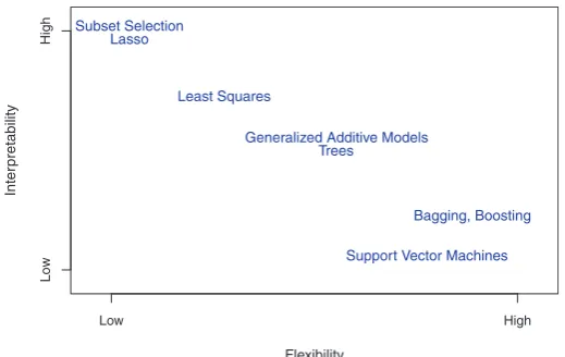
FIGURE 2.7. A representation of the tradeoﬀ between flexibility and

inter-pretability, using diﬀerent statistical learning methods. In general, as the flexibil-ity of a method increases, its interpretabilflexibil-ity decreases.

Other methods, such as the thin plate splines shown in Figures 2.5 and 2.6, are considerably more flexible because they can generate a much wider range of possible shapes to estimatef.

One might reasonably ask the following question: why would we ever choose to use a more restrictive method instead of a very flexible approach? There are several reasons that we might prefer a more restrictive model. If we are mainly interested in inference, then restrictive models are much more interpretable. For instance, when inference is the goal, the linear model may be a good choice since it will be quite easy to understand the relationship between Y and X1, X2, . . . , Xp. In contrast, very flexible approaches, such as the splines discussed in Chapter 7 and displayed in Figures 2.5 and 2.6, and the boosting methods discussed in Chapter 8, can lead to such complicated estimates of f that it is diﬃcult to understand how any individual predictor is associated with the response.

Figure 2.7 provides an illustration of the trade-oﬀ between flexibility and interpretability for some of the methods that we cover in this book. Least squares linear regression, discussed in Chapter 3, is relatively inflexible but is quite interpretable. The lasso, discussed in Chapter 6, relies upon the

lasso

(40)

additive models (GAMs), discussed in Chapter 7, instead extend the

lin-generalized additive model

ear model (2.4) to allow for certain non-linear relationships. Consequently, GAMs are more flexible than linear regression. They are also somewhat less interpretable than linear regression, because the relationship between each predictor and the response is now modeled using a curve. Finally, fully non-linear methods such asbagging,boosting, andsupport vector machines

bagging boosting

with non-linear kernels, discussed in Chapters 8 and 9, are highly flexible

support vector machine

approaches that are harder to interpret.

We have established that when inference is the goal, there are clear ad-vantages to using simple and relatively inflexible statistical learning meth-ods. In some settings, however, we are only interested in prediction, and the interpretability of the predictive model is simply not of interest. For instance, if we seek to develop an algorithm to predict the price of a stock, our sole requirement for the algorithm is that it predict accurately— interpretability is not a concern. In this setting, we might expect that it will be best to use the most flexible model available. Surprisingly, this is not always the case! We will often obtain more accurate predictions using a less flexible method. This phenomenon, which may seem counterintuitive at first glance, has to do with the potential for overfitting in highly flexible methods. We saw an example of overfitting in Figure 2.6. We will discuss this very important concept further in Section 2.2 and throughout this book.

2.1.4 Supervised Versus Unsupervised Learning

Most statistical learning problems fall into one of two categories:supervised _supervised or unsupervised. The examples that we have discussed so far in this chap- _unsupervised ter all fall into the supervised learning domain. For each observation of the

predictor measurement(s) xi, i= 1, . . . , n there is an associated response measurement yi. We wish to fit a model that relates the response to the predictors, with the aim of accurately predicting the response for future observations (prediction) or better understanding the relationship between the response and the predictors (inference). Many classical statistical learn-ing methods such as linear regression andlogistic regression(Chapter 4), as

logistic regression

well as more modern approaches such as GAM, boosting, and support vec-tor machines, operate in the supervised learning domain. The vast majority of this book is devoted to this setting.

(41)

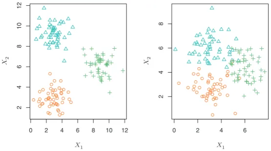
0 2 4 6 8 10 12

24

6

8

10

12

0 2 4 6

2468

FIGURE 2.8.A clustering data set involving three groups. Each group is shown

using a diﬀerent colored symbol. Left: The three groups are well-separated. In

this setting, a clustering approach should successfully identify the three groups.

Right:There is some overlap among the groups. Now the clustering task is more

challenging.

possible? We can seek to understand the relationships between the variables or between the observations. One statistical learning tool that we may use in this setting iscluster analysis, or clustering. The goal of cluster analysis

cluster analysis

is to ascertain, on the basis ofx1, . . . , xn, whether the observations fall into relatively distinct groups. For example, in a market segmentation study we might observe multiple characteristics (variables) for potential customers, such as zip code, family income, and shopping habits. We might believe that the customers fall into diﬀerent groups, such as big spenders versus low spenders. If the information about each customer’s spending patterns were available, then a supervised analysis would be possible. However, this information is not available—that is, we do not know whether each poten-tial customer is a big spender or not. In this setting, we can try to cluster the customers on the basis of the variables measured, in order to identify distinct groups of potential customers. Identifying such groups can be of interest because it might be that the groups diﬀer with respect to some property of interest, such as spending habits.

(42)

between the groups. A clustering method could not be expected to assign all of the overlapping points to their correct group (blue, green, or orange). In the examples shown in Figure 2.8, there are only two variables, and so one can simply visually inspect the scatterplots of the observations in order to identify clusters. However, in practice, we often encounter data sets that contain many more than two variables. In this case, we cannot easily plot the observations. For instance, if there are p variables in our data set, then p(p₋1)/2 distinct scatterplots can be made, and visual inspection is simply not a viable way to identify clusters. For this reason, automated clustering methods are important. We discuss clustering and other unsupervised learning approaches in Chapter 10.

Many problems fall naturally into the supervised or unsupervised learn-ing paradigms. However, sometimes the question of whether an analysis should be considered supervised or unsupervised is less clear-cut. For in-stance, suppose that we have a set ofnobservations. Formof the observa-tions, wherem < n, we have both predictor measurements and a response measurement. For the remaining n₋m observations, we have predictor measurements but no response measurement. Such a scenario can arise if the predictors can be measured relatively cheaply but the corresponding responses are much more expensive to collect. We refer to this setting as a semi-supervised learning problem. In this setting, we wish to use a sta-

semi-supervised learning

tistical learning method that can incorporate themobservations for which response measurements are available as well as then−mobservations for which they are not. Although this is an interesting topic, it is beyond the scope of this book.

2.1.5 Regression Versus Classification Problems

Variables can be characterized as either quantitative or qualitative (also _quantitative

qualitative

known as categorical). Quantitative variables take on numerical values.

categorical

Examples include a person’s age, height, or income, the value of a house, and the price of a stock. In contrast, qualitative variables take on val-ues in one of K diﬀerent classes, or categories. Examples of qualitative

class

variables include a person’s gender (male or female), the brand of prod-uct purchased (brand A, B, or C), whether a person defaults on a debt (yes or no), or a cancer diagnosis (Acute Myelogenous Leukemia, Acute Lymphoblastic Leukemia, or No Leukemia). We tend to refer to problems

with a quantitative response as regression problems, while those involv- _regression ing a qualitative response are often referred to as classificationproblems. _{classification} However, the distinction is not always that crisp. Least squares linear

re-gression (Chapter 3) is used with a quantitative response, whereas logistic regression (Chapter 4) is typically used with a qualitative (two-class, or binary) response. As such it is often used as a classification method. But

binary

(43)

method as well. Some statistical methods, such as K-nearest neighbors (Chapters 2 and 4) and boosting (Chapter 8), can be used in the case of either quantitative or qualitative responses.

We tend to select statistical learning methods on the basis of whether the response is quantitative or qualitative; i.e. we might use linear regres-sion when quantitative and logistic regresregres-sion when qualitative. However, whether the predictors are qualitative or quantitative is generally consid-ered less important. Most of the statistical learning methods discussed in this book can be applied regardless of the predictor variable type, provided that any qualitative predictors are properly coded before the analysis is performed. This is discussed in Chapter 3.

2.2 Assessing Model Accuracy

One of the key aims of this book is to introduce the reader to a wide range of statistical learning methods that extend far beyond the standard linear regression approach. Why is it necessary to introduce so many diﬀerent statistical learning approaches, rather than just a singlebestmethod?There is no free lunch in statistics: no one method dominates all others over all possible data sets. On a particular data set, one specific method may work best, but some other method may work better on a similar but diﬀerent data set. Hence it is an important task to decide for any given set of data which method produces the best results. Selecting the best approach can be one of the most challenging parts of performing statistical learning in practice.

In this section, we discuss some of the most important concepts that arise in selecting a statistical learning procedure for a specific data set. As the book progresses, we will explain how the concepts presented here can be applied in practice.

2.2.1 Measuring the Quality of Fit

In order to evaluate the performance of a statistical learning method on a given data set, we need some way to measure how well its predictions actually match the observed data. That is, we need to quantify the extent to which the predicted response value for a given observation is close to the true response value for that observation. In the regression setting, the most commonly-used measure is themean squared error(MSE), given by _mean

squared error

M SE = 1

n n

i=1

Springer Texts in Statistics