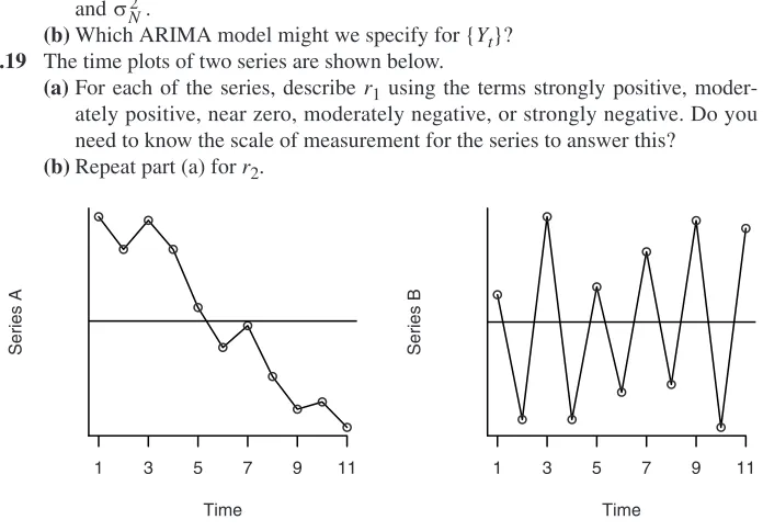
Statistics Texts in Statistics

Statistics Texts in Statistics

Series Editors:

Athreya/Lahiri: Measure Theory and Probability Theory Bilodeau/Brenner: Theory of Multivariate Statistics

Brockwell/Davis: An Introduction to Time Series and Forecasting Carmona: Statistical Analysis of Financial Data in S-PLUS

Chow/Teicher: Probability Theory: Independence, Interchangeability, Martingales, 3rd _ed. Christensen: Advanced Linear Modeling: Multivariate, Time Series, and Spatial Data; Nonparametric Regression and Response Surface Maximization, 2nd _ed.

Christensen: Log-Linear Models and Logistic Regression, 2nd ed.

Christensen: Plane Answers to Complex Questions: The Theory of Linear Models, 2nd _ed. Cryer/Chan: Time Series Analysis, Second Edition

Davis: Statistical Methods for the Analysis of Repeated Measurements Dean/Voss: Design and Analysis of Experiments

Dekking/Kraaikamp/Lopuhaä/Meester: A Modern Introduction to Probability and Statistics Durrett: Essential of Stochastic Processes

Edwards: Introduction to Graphical Modeling, 2nd ed.

Everitt: An R and S-PLUS Companion to Multivariate Analysis

Gentle: Matrix Algebra: Theory, Computations, and Applications in Statistics Ghosh/Delampady/Samanta: An Introduction to Bayesian Analysis

Gut: Probability: A Graduate Course in S-PLUS, R, and SAS

Jobson: Applied Multivariate Data Analysis, Volume I: Regression and Experimental Design Jobson: Applied Multivariate Data Analysis, Volume II: Categorical and Multivariate Methods Karr: Probability

Kulkarni: Modeling, Analysis, Design, and Control of Stochastic Systems Lange: Applied Probability

Lange: Optimization

Lehmann: Elements of Large Sample Theory

Lehmann/Romano: Testing Statistical Hypotheses, 3rd ed. Lehmann/Casella: Theory of Point Estimation, 2nd _ed.

Longford: Studying Human Popluations: An Advanced Course in Statistics

Marin/Robert: Bayesian Core: A Practical Approach to Computational Bayesian Statistics Nolan/Speed: Stat Labs: Mathematical Statistics Through Applications

Pitman: Probability

Rawlings/Pantula/Dickey: Applied Regression Analysis

Robert: The Bayesian Choice: From Decision-Theoretic Foundations to Computational Implementation, 2nd ed.

Robert/Casella: Monte Carlo Statistical Methods, 2nd ed. Rose/Smith: Mathematical Statistics with Mathematica Ruppert: Statistics and Finance: An Introduction

Sen/Srivastava: Regression Analysis: Theory, Methods, and Applications. Shao: Mathematical Statistics, 2nd ed.

Shorack: Probability for Statisticians

Shumway/Stoffer: Time Series Analysis and Its Applications, 2nd ed. Simonoff: Analyzing Categorical Data

Terrell: Mathematical Statistics: A Unified Introduction Timm: Applied Multivariate Analysis

Toutenberg: Statistical Analysis of Designed Experiments, 2nd ed. Wasserman: All of Nonparametric Statistics

Wasserman: All of Statistics: A Concise Course in Statistical Inference Weiss: Modeling Longitudinal Data

Whittle: Probability via Expectation, 4th ed.

Time Series Analysis

Jonathan D. Cryer • Kung-Sik Chan

With Applications in R

George Casella University of Florida USA

Department of Statistics Carnegie Mellon University

USA

Pittsburgh, PA 15213-3890

Ingram Okin

Department of Statistics

Stanford, CA 94305 USA

Series Editors: Department of Statistics

ISBN: 978-0-387-75958-6

© 2008 Springer Science+Business Media, LLC

Printed on acid-free paper.

9 8 7 6 5 4 3 2 1

springer.com

Stephen Fienberg

Stanford University

e-ISBN: 978-0-387-75959-3

All rights reserved. This work may not be translated or copied in whole or in part without the written permission of the publisher (Springer Science+Business Media, LLC, 233 Spring Street, New York, NY 10013, USA), except for brief excerpts in connection with reviews or scholarly analysis. Use in connection with any form of information storage and retrieval, electronic adaptation, computer software, or by similar or dissimilar methodology now known or hereafter developed is forbidden.

The use in this publication of trade names, trademarks, service marks, and similar terms, even if they are not identified as such, is not to be taken as an expression of opinion as to whether or not they are subject to proprietary rights.

Library of Congress Control Number: 2008923058

Gainesville, FL 32611-8545

Department of Statistics & Actuarial Science University of Iowa

Iowa City, Iowa 52242 USA

jon-cryer@uiowa.edu

Department of Statistics & Actuarial Science University of Iowa

Iowa City, Iowa 52242 USA

vii The theory and practice of time series analysis have developed rapidly since the appear-ance in 1970 of the seminal work of George E. P. Box and Gwilym M. Jenkins, Time Series Analysis: Forecasting and Control, now available in its third edition (1994) with co-author Gregory C. Reinsel. Many books on time series have appeared since then, but some of them give too little practical application, while others give too little theoretical background. This book attempts to present both application, and theory at a level acces-sible to a wide variety of students and practitioners. Our approach is to mix application and theory throughout the book as they are naturally needed.

The book was developed for a one-semester course usually attended by students in statistics, economics, business, engineering, and quantitative social sciences. Basic applied statistics through multiple linear regression is assumed. Calculus is assumed only to the extent of minimizing sums of squares, but a calculus-based introduction to statistics is necessary for a thorough understanding of some of the theory. However, required facts concerning expectation, variance, covariance, and correlation are reviewed in appendices. Also, conditional expectation properties and minimum mean square error prediction are developed in appendices. Actual time series data drawn from various disciplines are used throughout the book to illustrate the methodology. The book contains additional topics of a more advanced nature that can be selected for inclusion in a course if the instructor so chooses.

All of the plots and numerical output displayed in the book have been produced with the R software, which is available from the R Project for Statistical Computing at www.r-project.org. Some of the numerical output has been edited for additional clarity or for simplicity. R is available as free software under the terms of the Free Software Foundation's GNU General Public License in source code form. It runs on a wide vari-ety of UNIX platforms and similar systems, Windows, and MacOS.

R is a language and environment for statistical computing and graphics, provides a wide variety of statistical (e.g., time-series analysis, linear and nonlinear modeling, clas-sical statistical tests) and graphical techniques, and is highly extensible. The extensive appendix An Introduction to R, provides an introduction to the R software specially designed to go with this book. One of the authors (KSC) has produced a large number of new or enhanced R functions specifically tailored to the methods described in this book. They are listed on page 468 and are available in the package named TSA on the R Project’s Website at www.r-project.org. We have also constructed R command script files for each chapter. These are available for download at www.stat.uiowa.edu/ ~kchan/TSA.htm. We also show the required R code beneath nearly every table and graphical display in the book. The datasets required for the exercises are named in each exercise by an appropriate filename; for example, larain for the Los Angeles rainfall data. However, if you are using the TSA package, the datasets are part of the package and may be accessed through the R command data(larain), for example.

viii

described in the book could also be obtained with other software, such as SAS©_{, Splus}©_, Statgraphics©_{, SCA}©_{, EViews}©_{, RATS}©_{, Ox}©_{, and others.}

This book is a second edition of the book Time Series Analysis by Jonathan Cryer, published in 1986 by PWS-Kent Publishing (Duxbury Press). This new edition contains nearly all of the well-received original in addition to considerable new material, numer-ous new datasets, and new exercises. Some of the new topics that are integrated with the original include unit root tests, extended autocorrelation functions, subset ARIMA mod-els, and bootstrapping. Completely new chapters cover the topics of time series regres-sion models, time series models of heteroscedasticity, spectral analysis, and threshold models. Although the level of difficulty in these new chapters is somewhat higher than in the more basic material, we believe that the discussion is presented in a way that will make the material accessible and quite useful to a broad audience of users. Chapter 15, Threshold Models, is placed last since it is the only chapter that deals with nonlinear time series models. It could be covered earlier, say after Chapter 12. Also, Chapters 13 and 14 on spectral analysis could be covered after Chapter 10.

We would like to thank John Kimmel, Executive Editor, Statistics, at Springer, for his continuing interest and guidance during the long preparation of the manuscript. Pro-fessor Howell Tong of the London School of Economics, ProPro-fessor Henghsiu Tsai of Academica Sinica, Taipei, Professor Noelle Samia of Northwestern University, sor W. K. Li and Professor Kai W. Ng, both of the University of Hong Kong, and Profes-sor Nils Christian Stenseth of the University of Oslo kindly read parts of the manuscript, and Professor Jun Yan used a preliminary version of the text for a class at the University of Iowa. Their constructive comments are greatly appreciated. We would like to thank Samuel Hao who helped with the exercise solutions and read the appendix: An Introduc-tion to R. We would also like to thank several anonymous reviewers who read the manu-script at various stages. Their reviews led to a much improved book. Finally, one of the authors (JDC) would like to thank Dan, Marian, and Gene for providing such a great place, Casa de Artes, Club Santiago, Mexico, for working on the first draft of much of this new edition.

Iowa City, Iowa Jonathan D. Cryer

ix

CHAPTER 1 INTRODUCTION . . . 1

1.1

Examples of Time Series . . . 1

1.2

A Model-Building Strategy . . . 8

1.3

Time Series Plots in History . . . 8

1.4

An Overview of the Book . . . 9

Exercises . . . 10

CHAPTER 2 FUNDAMENTAL CONCEPTS . . . 11

2.1

Time Series and Stochastic Processes . . . 11

2.2

Means, Variances, and Covariances . . . 11

2.3

Stationarity . . . 16

2.4

Summary . . . 19

Exercises . . . 19

Appendix A: Expectation, Variance, Covariance, and Correlation . 24

CHAPTER 3 T

RENDS . . . 27

3.1

Deterministic Versus Stochastic Trends . . . 27

3.2

Estimation of a Constant Mean . . . 28

3.3

Regression Methods. . . 30

3.4

Reliability and Efficiency of Regression Estimates. . . 36

3.5

Interpreting Regression Output . . . 40

3.6

Residual Analysis . . . 42

3.7

Summary . . . 50

Exercises . . . 50

CHAPTER 4 MODELS FOR STATIONARY TIME SERIES . . . 55

4.1

General Linear Processes . . . 55

4.2

Moving Average Processes . . . 57

4.3

Autoregressive Processes . . . 66

4.4

The Mixed Autoregressive Moving Average Model. . . 77

4.5

Invertibility. . . 79

4.6

Summary . . . 80

Exercises . . . 81

Appendix B: The Stationarity Region for an AR(2) Process . . . 84

x Contents

CHAPTER 5 MODELS FOR NONSTATIONARY TIME SERIES . 87

5.1

Stationarity Through Differencing . . . 88

5.2

ARIMA Models. . . 92

5.3

Constant Terms in ARIMA Models. . . 97

5.4

Other Transformations . . . 98

5.5

Summary . . . .102

Exercises. . . .103

Appendix D: The Backshift Operator. . . .106

CHAPTER 6 MODEL SPECIFICATION . . . .109

6.1

Properties of the Sample Autocorrelation Function . . . .109

6.2

The Partial and Extended Autocorrelation Functions . . . . .112

6.3

Specification of Some Simulated Time Series. . . .117

6.4

Nonstationarity. . . .125

6.5

Other Specification Methods . . . .130

6.6

Specification of Some Actual Time Series. . . .133

6.7

Summary . . . .141

Exercises. . . .141

CHAPTER 7 PARAMETER ESTIMATION . . . .149

7.1

The Method of Moments . . . .149

7.2

Least Squares Estimation . . . .154

7.3

Maximum Likelihood and Unconditional Least Squares . . .158

7.4

Properties of the Estimates . . . .160

7.5

Illustrations of Parameter Estimation . . . .163

7.6

Bootstrapping ARIMA Models . . . .167

7.7

Summary . . . .170

Exercises. . . .170

CHAPTER 8 MODEL DIAGNOSTICS . . . .175

8.1

Residual Analysis . . . .175

8.2

Overfitting and Parameter Redundancy. . . .185

8.3

Summary . . . .188

CHAPTER 9 FORECASTING. . . 191

9.1

Minimum Mean Square Error Forecasting . . . 191

9.2

Deterministic Trends . . . 191

9.3

ARIMA Forecasting . . . 193

9.4

Prediction Limits . . . 203

9.5

Forecasting Illustrations . . . 204

9.6

Updating ARIMA Forecasts . . . 207

9.7

Forecast Weights and Exponentially Weighted

Moving Averages . . . 207

9.8

Forecasting Transformed Series. . . 209

9.9

Summary of Forecasting with Certain ARIMA Models . . . . 211

9.10 Summary . . . 213

Exercises . . . 213

Appendix E: Conditional Expectation. . . 218

Appendix F: Minimum Mean Square Error Prediction . . . 218

Appendix G: The Truncated Linear Process . . . 221

Appendix H: State Space Models . . . 222

CHAPTER 10 SEASONAL MODELS . . . 227

10.1 Seasonal ARIMA Models . . . 228

10.2 Multiplicative Seasonal ARMA Models . . . 230

10.3 Nonstationary Seasonal ARIMA Models . . . 233

10.4 Model Specification, Fitting, and Checking. . . 234

10.5 Forecasting Seasonal Models . . . 241

10.6 Summary . . . 246

Exercises . . . 246

CHAPTER 11 TIME SERIES REGRESSION MODELS . . . 249

11.1 Intervention Analysis . . . 249

11.2 Outliers . . . 257

11.3 Spurious Correlation. . . 260

11.4 Prewhitening and Stochastic Regression . . . 265

11.5 Summary . . . 273

xii Contents

CHAPTER 12 TIME SERIES MODELS OF

HETEROSCEDASTICITY. . . .277

12.1 Some Common Features of Financial Time Series . . . .278

12.2 The ARCH(1) Model . . . .285

12.3 GARCH Models . . . .289

12.4 Maximum Likelihood Estimation . . . .298

12.5 Model Diagnostics . . . .301

12.6 Conditions for the Nonnegativity of the

Conditional Variances . . . .307

12.7 Some Extensions of the GARCH Model . . . .310

12.8 Another Example: The Daily USD/HKD Exchange Rates . .311

12.9 Summary . . . .315

Exercises. . . .316

Appendix I: Formulas for the Generalized Portmanteau Tests . . .318

CHAPTER 13 INTRODUCTION TO SPECTRAL ANALYSIS. . . .319

13.1 Introduction . . . .319

13.2 The Periodogram . . . .322

13.3 The Spectral Representation and Spectral Distribution . . . .327

13.4 The Spectral Density . . . .330

13.5 Spectral Densities for ARMA Processes . . . .332

13.6 Sampling Properties of the Sample Spectral Density . . . . .340

13.7 Summary . . . .346

Exercises. . . .346

Appendix J: Orthogonality of Cosine and Sine Sequences . . . . .349

CHAPTER 14 ESTIMATING THE SPECTRUM . . . .351

14.1 Smoothing the Spectral Density . . . .351

14.2 Bias and Variance . . . .354

14.3 Bandwidth . . . .355

14.4 Confidence Intervals for the Spectrum . . . .356

14.5 Leakage and Tapering . . . .358

14.6 Autoregressive Spectrum Estimation. . . .363

14.7 Examples with Simulated Data . . . .364

14.8 Examples with Actual Data . . . .370

14.9 Other Methods of Spectral Estimation . . . .376

14.10 Summary . . . .378

Exercises. . . .378

CHAPTER 15 THRESHOLD MODELS . . . 383

15.1 Graphically Exploring Nonlinearity . . . 384

15.2 Tests for Nonlinearity . . . 390

15.3 Polynomial Models Are Generally Explosive . . . 393

15.4 First-Order Threshold Autoregressive Models . . . 395

15.5 Threshold Models . . . 399

15.6 Testing for Threshold Nonlinearity . . . 400

15.7 Estimation of a TAR Model . . . 402

15.8 Model Diagnostics . . . 411

15.9 Prediction . . . 415

15.10 Summary . . . 420

Exercises . . . 420

Appendix L: The Generalized Portmanteau Test for TAR . . . 421

Introduction . . . 423

Chapter 1 R Commands . . . 429

Chapter 2 R Commands . . . 433

Chapter 3 R Commands . . . 433

Chapter 4 R Commands . . . 438

Chapter 5 R Commands . . . 439

Chapter 6 R Commands . . . 441

Chapter 7 R Commands . . . 442

Chapter 8 R Commands . . . 446

Chapter 9 R Commands . . . 447

Chapter 10 R Commands . . . 450

Chapter 11 R Commands . . . 451

Chapter 12 R Commands . . . 457

Chapter 13 R Commands . . . 460

Chapter 14 R Commands . . . 461

Chapter 15 R Commands . . . 462

New or Enhanced Functions in the TSA Library . . . 468

DATASET INFORMATION . . . .

471

BIBLIOGRAPHY . . . 477

INDEX . . . 487

423

. . .

1

C

HAPTER

1

I

NTRODUCTION

Data obtained from observations collected sequentially over time are extremely com-mon. In business, we observe weekly interest rates, daily closing stock prices, monthly price indices, yearly sales figures, and so forth. In meteorology, we observe daily high and low temperatures, annual precipitation and drought indices, and hourly wind speeds. In agriculture, we record annual figures for crop and livestock production, soil erosion, and export sales. In the biological sciences, we observe the electrical activity of the heart at millisecond intervals. In ecology, we record the abundance of an animal spe-cies. The list of areas in which time series are studied is virtually endless. The purpose of time series analysis is generally twofold: to understand or model the stochastic mech-anism that gives rise to an observed series and to predict or forecast the future values of a series based on the history of that series and, possibly, other related series or factors.

This chapter will introduce a variety of examples of time series from diverse areas of application. A somewhat unique feature of time series and their models is that we usually cannot assume that the observations arise independently from a common popu-lation (or from popupopu-lations with different means, for example). Studying models that incorporate dependence is the key concept in time series analysis.

1.1

Examples of Time Series

In this section, we introduce a number of examples that will be pursued in later chapters.

Annual Rainfall in Los Angeles

Exhibit 1.1 displays a time series plot of the annual rainfall amounts recorded in Los Angeles, California, over more than 100 years. The plot shows considerable variation in rainfall amount over the years — some years are low, some high, and many are in-between in value. The year 1883 was an exceptionally wet year for Los Angeles, while 1983 was quite dry. For analysis and modeling purposes we are interested in whether or not consecutive years are related in some way. If so, we might be able to use one year’s rainfall value to help forecast next year’s rainfall amount. One graphical way to investigate that question is to pair up consecutive rainfall values and plot the resulting scatterplot of pairs.

near the top of the display shows that the 40 inch year was preceded by a much more typical year of about 15 inches.

Exhibit 1.1 Time Series Plot of Los Angeles Annual Rainfall

> library(TSA)

> win.graph(width=4.875, height=2.5,pointsize=8)

> data(larain); plot(larain,ylab='Inches',xlab='Year',type='o')

Exhibit 1.2 Scatterplot of LA Rainfall versus Last Year’s LA Rainfall

> win.graph(width=3,height=3,pointsize=8) > plot(y=larain,x=zlag(larain),ylab='Inches',

xlab='Previous Year Inches')

●●

1880 1900 1920 1940 1960 1980

10

Previous Year Inches

1.1 Examples of Time Series 3

The main impression that we obtain from this plot is that there is little if any infor-mation about this year’s rainfall amount from last year’s amount. The plot shows no “trends” and no general tendencies. There is little correlation between last year’s rainfall amount and this year’s amount. From a modeling or forecasting point of view, this is not a very interesting time series!

An Industrial Chemical Process

As a second example, we consider a time series from an industrial chemical process. The variable measured here is a color property from consecutive batches in the process. Exhibit 1.3 shows a time series plot of these color values. Here values that are neighbors in time tend to be similar in size. It seems that neighbors are related to one another.

Exhibit 1.3 Time Series Plot of Color Property from a Chemical Process

> win.graph(width=4.875, height=2.5,pointsize=8) > data(color)

> plot(color,ylab='Color Property',xlab='Batch',type='o')

This can be seen better by constructing the scatterplot of neighboring pairs as we did with the first example.

Exhibit 1.4 displays the scatterplot of the neighboring pairs of color values. We see a slight upward trend in this plot—low values tend to be followed in the next batch by low values, middle-sized values tend to be followed by middle-sized values, and high values tend to be followed by high values. The trend is apparent but is not terribly strong. For example, the correlation in this scatterplot is about 0.6.

● ●

●

● ●

● ● ● ● ● ●

●

● ●

● ●

● ●

● ● ●

● ● ●

● ● ● ●

● ●

● ● ●

●

●

Batch

Color Property

0 5 10 15 20 25 30 35

65

75

Exhibit 1.4 Scatterplot of Color Value versus Previous Color Value

> win.graph(width=3,height=3,pointsize=8)

> plot(y=color,x=zlag(color),ylab='Color Property', xlab='Previous Batch Color Property')

Annual Abundance of Canadian Hare

Our third example concerns the annual abundance of Canadian hare. Exhibit 1.5 gives the time series plot of this abundance over about 30 years. Neighboring values here are very closely related. Large changes in abundance do not occur from one year to the next. This neighboring correlation is seen clearly in Exhibit 1.6 where we have plotted abun-dance versus the previous year’s abunabun-dance. As in the previous example, we see an upward trend in the plot—low values tend to be followed by low values in the next year, middle-sized values by middle-sized values, and high values by high values.

● ●

● ●

● ●

● ● ● ●

●

● ●

● ●

● ●

● ●

●

● ●

●

●

●

● ●

● ●

● ● ●

●

●

65 70 75 80 85

65

70

75

80

85

Previous Batch Color Property

1.1 Examples of Time Series 5

Exhibit 1.5 Abundance of Canadian Hare

> win.graph(width=4.875, height=2.5,pointsize=8)

> data(hare); plot(hare,ylab='Abundance',xlab='Year',type='o')

Exhibit 1.6 Hare Abundance versus Previous Year’s Hare Abundance

> win.graph(width=3, height=3,pointsize=8) > plot(y=hare,x=zlag(hare),ylab='Abundance',

xlab='Previous Year Abundance')

●

● ● ● ● ● ●

● ●

●

● ●

● ● ●

● ●

● ● ●

● ●

● ● ● ●

● ●

● ●

●

Year

Abundance

1905 1910 1915 1920 1925 1930 1935

04

0

8

0

● ●

● ●

●

● ●

●

●

● ●

● ● ●

● ●

● ●

●

●

● ● ● ●●

●

●

●

●

●

0 20 40 60 80

0

2

04

06

08

0

Previous Year Abundance

Monthly Average Temperatures in Dubuque, Iowa

The average monthly temperatures (in degrees Fahrenheit) over a number of years recorded in Dubuque, Iowa, are shown in Exhibit 1.7.

Exhibit 1.7 Average Monthly Temperatures, Dubuque, Iowa

> win.graph(width=4.875, height=2.5,pointsize=8)

> data(tempdub); plot(tempdub,ylab='Temperature',type='o')

This time series displays a very regular pattern called seasonality. Seasonality for monthly values occurs when observations twelve months apart are related in some man-ner or another. All Januarys and Februarys are quite cold but they are similar in value and different from the temperatures of the warmer months of June, July, and August, for example. There is still variation among the January values and variation among the June values. Models for such series must accommodate this variation while preserving the similarities. Here the reason for the seasonality is well understood — the Northern Hemisphere’s changing inclination toward the sun.

Monthly Oil Filter Sales

Our last example for this chapter concerns the monthly sales to dealers of a specialty oil filter for construction equipment manufactured by John Deere. When these data were first presented to one of the authors, the manager said, “There is no reason to believe that these sales are seasonal.” Seasonality would be present if January values tended to be related to other January values, February values tended to be related to other Febru-ary values, and so forth. The time series plot shown in Exhibit 1.8 is not designed to dis-play seasonality especially well. Exhibit 1.9 gives the same plot but amended to use meaningful plotting symbols. In this plot, all January values are plotted with the charac-ter J, all Februarys with F, all Marches with M, and so forth.† With these plotting sym-bols, it is much easier to see that sales for the winter months of January and February all tend to be high, while sales in September, October, November, and December are

gener-●●

1964 1966 1968 1970 1972 1974 1976

10

30

50

1.1 Examples of Time Series 7

ally quite low. The seasonality in the data is much easier to see from this modified time series plot.

Exhibit 1.8 Monthly Oil Filter Sales

> data(oilfilters); plot(oilfilters,type='o',ylab='Sales')

Exhibit 1.9 Monthly Oil Filter Sales with Special Plotting Symbols

> plot(oilfilters,type='l',ylab='Sales') > points(y=oilfilters,x=time(oilfilters),

pch=as.vector(season(oilfilters)))

† _{In reading the plot, you will still have to distinguish between Januarys, Junes, and Julys,} between Marches and Mays, and Aprils and Augusts, but this is easily done by looking at neighboring plotting characters.

● ●

● ●

● ●

●

● ● ● ● ●

●

● ●

● ●

● ●

●

● ●

● ● ●

● ●

● ● ●

● ●

● ●

● ●

● ●

● ● ●

● ●

●

● ●

●

●

Time

Sales

1984 1985 1986 1987

2000

4000

6000

Time

Sales

1984 1985 1986 1987

2000

4000

6000

J A

S

O

N D

J

FMAM J

J

A

SO_N D

J F

M AMJ

J

A

S ON

D J

F

M A

M J

J

A

S ON

D J

F

M A

M

J

J=January (and June and July),

In general, our goal is to emphasize plotting methods that are appropriate and use-ful for finding patterns that will lead to suitable models for our time series data. In later chapters, we will consider several different ways to incorporate seasonality into time series models.

1.2

A Model-Building Strategy

Finding appropriate models for time series is a nontrivial task. We will develop a multi-step model-building strategy espoused so well by Box and Jenkins (1976). There are three main steps in the process, each of which may be used several times:

1. model specification (or identification) 2. model fitting, and

3. model diagnostics

In model specification (or identification), the classes of time series models are selected that may be appropriate for a given observed series. In this step we look at the time plot of the series, compute many different statistics from the data, and also apply any knowledge of the subject matter in which the data arise, such as biology, business, or ecology. It should be emphasized that the model chosen at this point is tentative and subject to revision later on in the analysis.

In choosing a model, we shall attempt to adhere to the principle of parsimony; that is, the model used should require the smallest number of parameters that will adequately represent the time series. Albert Einstein is quoted in Parzen (1982, p. 68) as remarking that “everything should be made as simple as possible but not simpler.”

The model will inevitably involve one or more parameters whose values must be estimated from the observed series. Model fitting consists of finding the best possible estimates of those unknown parameters within a given model. We shall consider criteria such as least squares and maximum likelihood for estimation.

Model diagnostics is concerned with assessing the quality of the model that we have specified and estimated. How well does the model fit the data? Are the assump-tions of the model reasonably well satisfied? If no inadequacies are found, the modeling may be assumed to be complete, and the model may be used, for example, to forecast future values. Otherwise, we choose another model in the light of the inadequacies found; that is, we return to the model specification step. In this way, we cycle through the three steps until, ideally, an acceptable model is found.

Because the computations required for each step in model building are intensive, we shall rely on readily available statistical software to carry out the calculations and do the plotting.

1.3

Time Series Plots in History

sec-1.4 An Overview of the Book 9

onds, minutes, hours, days, weeks, months, years, or millennia, the natural ordering of the time scale gives this design a strength and efficiency of interpretation found in no other graphic arrangement.”

Exhibit 1.10 reproduces what appears to be the oldest known example of a time series plot, dating from the tenth (or possibly eleventh) century and showing the inclina-tions of the planetary orbits.† Commenting on this artifact, Tufte says “It appears as a mysterious and isolated wonder in the history of data graphics, since the next extant graphic of a plotted time-series shows up some 800 years later.”

Exhibit 1.10 A Tenth-Century Time Series Plot

1.4

An Overview of the Book

Chapter 2 develops the basic ideas of mean, covariance, and correlation functions and ends with the important concept of stationarity. Chapter 3 discusses trend analysis and investigates how to estimate and check common deterministic trend models, such as those for linear time trends and seasonal means.

Chapter 4 begins the development of parametric models for stationary time series, namely the so-called autoregressive moving average (ARMA) models (also known as Box-Jenkins models). These models are then generalized in Chapter 5 to encompass certain types of stochastic nonstationary cases—the ARIMA models.

Chapters 6, 7, and 8 form the heart of the model-building strategy for ARIMA mod-eling. Techniques are presented for tentatively specifying models (Chapter 6), effi-ciently estimating the model parameters using least squares and maximum likelihood (Chapter 7), and determining how well the models fit the data (Chapter 8).

Chapter 9 thoroughly develops the theory and methods of minimum mean square error forecasting for ARIMA models. Chapter 10 extends the ideas of Chapters 4

through 9 to stochastic seasonal models. The remaining chapters cover selected topics and are of a somewhat more advanced nature.

E

XERCISES

1.1 Use software to produce the time series plot shown in Exhibit 1.2, on page 2. The data are in the file named larain.†

1.2 Produce the time series plot displayed in Exhibit 1.3, on page 3. The data file is named color.

1.3 Simulate a completely random process of length 48 with independent, normal val-ues. Plot the time series plot. Does it look “random”? Repeat this exercise several times with a new simulation each time.

1.4 Simulate a completely random process of length 48 with independent, chi-square distributed values, each with 2 degrees of freedom. Display the time series plot. Does it look “random” and nonnormal? Repeat this exercise several times with a new simulation each time.

1.5 Simulate a completely random process of length 48 with independent, t -distrib-uted values each with 5 degrees of freedom. Construct the time series plot. Does it look “random” and nonnormal? Repeat this exercise several times with a new simulation each time.

1.6 Construct a time series plot with monthly plotting symbols for the Dubuque tem-perature series as in Exhibit 1.9, on page 7. The data are in the file named temp-dub.

11

C

HAPTER

2

F

UNDAMENTAL

C

ONCEPTS

This chapter describes the fundamental concepts in the theory of time series models. In particular, we introduce the concepts of stochastic processes, mean and covariance func-tions, stationary processes, and autocorrelation functions.

2.1

Time Series and Stochastic Processes

The sequence of random variables {Y_t: t = 0, ±1, ±2, ±3,…} is called a stochastic process and serves as a model for an observed time series. It is known that the complete probabilistic structure of such a process is determined by the set of distributions of all finite collections of the Y’s. Fortunately, we will not have to deal explicitly with these multivariate distributions. Much of the information in these joint distributions can be described in terms of means, variances, and covariances. Consequently, we concentrate our efforts on these first and second moments. (If the joint distributions of the Y’s are multivariate normal distributions, then the first and second moments completely deter-mine all the joint distributions.)

2.2

Means, Variances, and Covariances

For a stochastic process {Y_t: t = 0, ±1, ±2, ±3,…}, the mean function is defined by (2.2.1)

That is, μ_t is just the expected value of the process at time t. In general, μ_t can be differ-ent at each time point t.

The autocovariance function, γ_t,s, is defined as

(2.2.2)

where Cov(Y_t, Y_s) = E[(Y_t−μ_t)(Y_s−μ_s)] = E(Y_tY_s) −μ_tμ_s. The autocorrelation function, ρ_t,s, is given by

(2.2.3)

where

(2.2.4) μ_t = E Y( )_t for t = 0, 1± ,±2 ...,

γ_{t s,} = Cov Y( _t,Y_s) for t s, = 0, 1± ,±2 ...,

ρ_{t s,} = Corr Y( _t,Y_s) for t s, = 0, 1± ,±2 ...,

Corr Y( _t,Y_s) Cov Y( t,Ys) Var Y( )_t Var Y( )_s

--- γt s, γ_{t t,} γ_{s s,}

We review the basic properties of expectation, variance, covariance, and correlation in Appendix A on page 24.

Recall that both covariance and correlation are measures of the (linear) dependence between random variables but that the unitless correlation is somewhat easier to inter-pret. The following important properties follow from known results and our definitions:

(2.2.5)

Values of ρ_t,s near ±1 indicate strong (linear) dependence, whereas values near zero indicate weak (linear) dependence. If ρ_t,s = 0, we say that Y_t and Y_s are uncorrelated.

To investigate the covariance properties of various time series models, the follow-ing result will be used repeatedly: If c₁, c₂,…, c_m and d₁, d₂,…, d_n are constants and t₁,

t₂,…, t_m and s₁, s₂,…, s_n are time points, then

(2.2.6)

The proof of Equation (2.2.6), though tedious, is a straightforward application of the linear properties of expectation. As a special case, we obtain the well-known result

(2.2.7)

The Random Walk

Let e₁, e₂,… be a sequence of independent, identically distributed random variables each with zero mean and variance . The observed time series, {Y_t: t = 1, 2,…}, is constructed as follows:

(2.2.8)

Alternatively, we can write

(2.2.9)

with “initial condition” Y₁ = e₁. If the e’s are interpreted as the sizes of the “steps” taken (forward or backward) along a number line, then Y_t is the position of the “random walker” at time t. From Equation (2.2.8), we obtain the mean function

γ_{t t,} = Var Y( )_t γ_{t s,} = γ_{s t,}

γ_{t s,} ≤ γ_{t t,} γ_{s s,}

ρ_{t t,} = 1 ρ_{t s,} = ρ_{s t,}

ρ_{t s,} ≤1 _⎭⎪ ⎬ ⎪ ⎫

Cov c_iY_t

i

i=1

m

∑

d_jY_s

j

j=1

n

∑

, c_id_jCov Y_t

i,Ysj

( )

j=1

n

∑

i=1

m

∑

=

Var c_iY_t

i

i=1

n

∑

c_i2Var Y_t

i

( )

i=1

n

∑

2 c_ic_jCov Y_t

i,Ytj

( )

j=1

i–1

∑

i=2

n

∑

+ =

σ_e2

Y₁ = e₁ Y₂ = e₁+e₂

...

Y_t = e₁+e₂+…+e_t

⎭ ⎪ ⎪ ⎬ ⎪ ⎪ ⎫

2.2 Means, Variances, and Covariances 13

so that

μ_t = 0 for all t (2.2.10) We also have

so that

(2.2.11)

Notice that the process variance increases linearly with time.

To investigate the covariance function, suppose that 1 ≤ t ≤s. Then we have

From Equation (2.2.6), we have

However, these covariances are zero unless i = j, in which case they equal Var(e_i) = . There are exactly t of these so that γ_t,s = t .

Since γ_t,s = γ_s,t, this specifies the autocovariance function for all time points t and s

and we can write

(2.2.12)

The autocorrelation function for the random walk is now easily obtained as

(2.2.13)

The following numerical values help us understand the behavior of the random walk.

The values of Y at neighboring time points are more and more strongly and posi-tively correlated as time goes by. On the other hand, the values of Y at distant time points are less and less correlated.

A simulated random walk is shown in Exhibit 2.1 where the e’s were selected from a standard normal distribution. Note that even though the theoretical mean function is

μ_t = E Y( )_t = E e( ₁+e₂+…+e_t) = E e( )₁ +E e( ) …₂ + +E e( )_t

0+0+…+0 =

Var Y( )_t = Var e( ₁+e₂+…+e_t) = Var e( )₁ +Var e( ) …₂ + +Var e( )_t

σ_e2 _σ

e2 … σe2

+ + +

=

Var Y( )_{t =} tσ_e2

γ_{t s,} = Cov Y( _t,Y_s) = Cov e( ₁+e₂+…+e_t,e₁+e₂+…+e_t+e_t+1+…+e_s)

γ_{t s,} Cov e( _i,e_j)

j=1

t

∑

i=1

s

∑

=

σ_e2

σ_e2

γ_{t s,} = tσ_e2 for 1≤ ≤t s

ρ_{t s,} γt s,

γ_{t t,} γ_{s s,} --- t

s

--= = for 1≤ ≤t s

ρ_{1 2,} 1 2

--- 0.707

= =

ρ_{24 25,} 24

25

--- 0.980

= =

ρ_{8 9,} 8 9

--- 0.943

= =

ρ_{1 25,} 1 25

--- 0.200

zero for all time points, the fact that the variance increases over time and that the corre-lation between process values nearby in time is nearly 1 indicate that we should expect long excursions of the process away from the mean level of zero.

The simple random walk process provides a good model (at least to a first approxi-mation) for phenomena as diverse as the movement of common stock price, and the position of small particles suspended in a fluid—so-called Brownian motion.

Exhibit 2.1 Time Series Plot of a Random Walk

> win.graph(width=4.875, height=2.5,pointsize=8) > data(rwalk) # rwalk contains a simulated random walk > plot(rwalk,type='o',ylab='Random Walk')

A Moving Average

As a second example, suppose that {Y_t} is constructed as

(2.2.14)

where (as always throughout this book) the e’s are assumed to be independent and iden-tically distributed with zero mean and variance . Here

and

●●● ●

● ●

● ●

● ●

● ● ● ●

● ● ●

● ●

● ●

● ● ●

● ● ●

● ●●●

● ●●

● ●

● ●

● ● ●

● ●●

●

● ●

● ●

●● ●

● ●

● ●●

● ● ●

Time

Random Walk

0 10 20 30 40 50 60

−

2

02468

Y_t et+et–1

2 ---=

σ_e2

μ_t E Y( )_t E et+et–1

2

---⎩ ⎭

⎨ ⎬

⎧ ⎫ E e( )_t +E e( _t–1)

2

---= = =

2.2 Means, Variances, and Covariances 15

Also

or

(2.2.15)

Furthermore,

Similarly, Cov(Y_t, Y_t−k) = 0 for k > 1, so we may write

For the autocorrelation function, we have

(2.2.16)

since 0.25 /0.5 = 0.5.

Notice that ρ_2,1 = ρ_3,2 = ρ_4,3 = ρ_9,8 = 0.5. Values of Y precisely one time unit apart have exactly the same correlation no matter where they occur in time. Furthermore, ρ_3,1 = ρ_4,2 = ρ_{t,t − 2} and, more generally, ρ_{t,t − k}is the same for all values of t. This leads us to the important concept of stationarity.

Var Y( )_t Var et+et–1

2

---⎩ ⎭

⎨ ⎬

⎧ ⎫ Var e( )_t +Var e( _t–1)

4

---= =

0.5σ_e2 =

Cov Y( _t,Y_t–1) Cov et+et–1

2

--- et–1+et–2 2 ---,

⎩ ⎭

⎨ ⎬

⎧ ⎫

=

Cov e( _t,e_t–1)+Cov e( _t,e_t–2)+Cov e( _t–1,e_t–1)

4

---=

Cov e( _t–1,e_t–2)

4 ---+

Cov e( _t–1,e_t–1)

4

---= (as all the other covariances are zero)

0.25σ_e2

=

γ_{t t, –1} = 0.25σ_e2 for all t

Cov Y( _t,Y_t–2) Cov et+et–1

2

--- et–2+et–3 2 ---,

⎩ ⎭

⎨ ⎬

⎧ ⎫

=

0

= since the e′s are independent.

γ_{t s,}

0.5σ_e2 _{for t s– = 0}

0.25σ_e2 for t s– = 1 0 for t s– >1 ⎩

⎪ ⎪ ⎨ ⎪ ⎪ ⎧

=

ρ_{t s, 0.5 for} 1 for t_t–_–s_s =₌ 0₁ 0 for t–s >1 ⎩

⎪ ⎨ ⎪ ⎧ =

σ_e2 _σ

2.3

Stationarity

To make statistical inferences about the structure of a stochastic process on the basis of an observed record of that process, we must usually make some simplifying (and pre-sumably reasonable) assumptions about that structure. The most important such assumption is that of stationarity. The basic idea of stationarity is that the probability laws that govern the behavior of the process do not change over time. In a sense, the pro-cess is in statistical equilibrium. Specifically, a propro-cess {Y_t} is said to be strictly sta-tionary if the joint distribution of is the same as the joint distribution of for all choices of time points t₁, t₂,…, t_n and all choices of time lag k.

Thus, when n = 1 the (univariate) distribution of Y_t is the same as that of Y_{t − k} for all t and k; in other words, the Y’s are (marginally) identically distributed. It then follows that E(Y_t) = E(Y_{t − k}) for all t and k so that the mean function is constant for all time. Additionally, Var(Y_t) = Var(Y_{t − k}) for all t and k so that the variance is also constant over time.

Setting n = 2 in the stationarity definition we see that the bivariate distribution of Y_t

and Y_s must be the same as that of Y_t−k and Y_s−k from which it follows that Cov(Y_t, Y_s) = Cov(Y_{t − k}, Y_{s − k}) for all t, s, and k. Putting k = s and then k = t, we obtain

That is, the covariance between Y_t and Y_s depends on time only through the time differ-ence |t − s| and not otherwise on the actual times t and s. Thus, for a stationary process, we can simplify our notation and write

(2.3.1)

Note also that

The general properties given in Equation (2.2.5) now become

(2.3.2)

If a process is strictly stationary and has finite variance, then the covariance func-tion must depend only on the time lag.

A definition that is similar to that of strict stationarity but is mathematically weaker

Yt₁,Yt₂,…,Yt_n Y_t

1–k Yt2–k,…,Ytn–k

γ_{t s,} = Cov Y( _t–s,Y₀) Cov Y( ₀,Y_s–t)

=

Cov Y( ₀,Y_t–s)

= γ_{0, t–s} =

γ_k = Cov Y( _t,Y_t–k) and ρ_k = Corr Y( _t,Y_t–k)

ρ_k γk

γ₀ ---=

γ₀ = Var Y( )_t

γ_k = γ_–k γ_k ≤γ₀

ρ₀ = 1 ρ_k = ρ_–k

2.3 Stationarity 17

is the following: A stochastic process {Y_t} is said to be weakly (or second-order)

stationary if

In this book the term stationary when used alone will always refer to this weaker form of stationarity. However, if the joint distributions for the process are all multivariate normal distributions, it can be shown that the two definitions coincide. For stationary processes, we usually only consider k≥ 0.

White Noise

A very important example of a stationary process is the so-called white noise process, which is defined as a sequence of independent, identically distributed random variables {e_t}. Its importance stems not from the fact that it is an interesting model itself but from the fact that many useful processes can be constructed from white noise. The fact that {e_t} is strictly stationary is easy to see since

as required. Also, μ_t = E(e_t) is constant and

Alternatively, we can write

(2.3.3)

The term white noise arises from the fact that a frequency analysis of the model shows that, in analogy with white light, all frequencies enter equally. We usually assume that the white noise process has mean zero and denote Var(e_t) by .

The moving average example, on page 14, where Y_t = (e_t + e_{t − 1})/2, is another example of a stationary process constructed from white noise. In our new notation, we have for the moving average process that

1. 2.

The mean function is constant over time, and

γ_{t t k, –} = γ_0,k for all time t and lag k

Pr e_t

1≤x1,et2≤x2,…,etn≤xn

( )

Pr e_t

1≤x1 ( )Pr e_t

2≤x2

( )…Pr e_t

n≤xn

( )

= (by independence)

Pr e_t

1–k≤x1

( )Pr e_t

2–k≤x2

( )…Pr e_t

n–k≤xn

( )

=

(identical distributions)

Pr e_t

1–k≤x1,et2–k≤x2,…,etn–k≤xn

( )

= (by independence)

γ_k Var e( )t

0 ⎩ ⎨ ⎧

= for k = 0

for k≠0

ρ_k 1

0 ⎩ ⎨ ⎧

= for k = 0 for k≠0

σ_e2

ρ_k 1 0.5

0 ⎩ ⎪ ⎨ ⎪ ⎧ =

Random Cosine Wave

As a somewhat different example,† consider the process defined as follows:

where Φ is selected (once) from a uniform distribution on the interval from 0 to 1. A sample from such a process will appear highly deterministic since Y_t will repeat itself identically every 12 time units and look like a perfect (discrete time) cosine curve. How-ever, its maximum will not occur at t = 0 but will be determined by the random phase Φ. The phase Φ can be interpreted as the fraction of a complete cycle completed by time t = 0. Still, the statistical properties of this process can be computed as follows:

But this is zero since the sines must agree. So μ_t = 0 for all t. Also

† _{This example contains optional material that is not needed in order to understand most of} the remainder of this book. It will be used in Chapter 13, Introduction to Spectral Analysis.

2.4 Summary 19

So the process is stationary with autocorrelation function

(2.3.4)

This example suggests that it will be difficult to assess whether or not stationarity is a reasonable assumption for a given time series on the basis of the time sequence plot of the observed data.

The random walk of page 12, where , is also constructed from white noise but is not stationary. For example, the variance function, Var(Y_t) =

t , is not constant; furthermore, the covariance function for 0 ≤t≤s does not depend only on time lag. However, suppose that instead of analyzing {Y_t} directly, we consider the differences of successive Y-values, denoted ∇Y_t. Then ∇Y_t= Y_t−Y_t−1 =

e_t, so the differenced series, {∇Y_t}, is stationary. This represents a simple example of a technique found to be extremely useful in many applications. Clearly, many real time series cannot be reasonably modeled by stationary processes since they are not in statis-tical equilibrium but are evolving over time. However, we can frequently transform non-stationary series into non-stationary series by simple techniques such as differencing. Such techniques will be vigorously pursued in the remaining chapters.

2.4

Summary

In this chapter we have introduced the basic concepts of stochastic processes that serve as models for time series. In particular, you should now be familiar with the important concepts of mean functions, autocovariance functions, and autocorrelation functions. We illustrated these concepts with the basic processes: the random walk, white noise, a simple moving average, and a random cosine wave. Finally, the fundamental concept of stationarity introduced here will be used throughout the book.

E

XERCISES

2.1 Suppose E(X) = 2, Var(X) = 9, E(Y) = 0, Var(Y) = 4, and Corr(X,Y) = 0.25. Find:

(a)Var(X + Y).

(b)Cov(X, X + Y).

(c)Corr(X + Y, X− Y).

2.2 If X and Y are dependent but Var(X) = Var(Y), find Cov(X + Y, X−Y).

2.3 Let X have a distribution with mean μ and variance σ2, and let Y_t = X for all t.

(a)Show that {Y_t} is strictly and weakly stationary.

(b)Find the autocovariance function for {Y_t}.

(c)Sketch a “typical” time plot of Y_t.

ρ_k 2π k

12

---⎝ ⎠

⎛ ⎞

cos

= for k = 0,±1,±2,…

Y_t = e₁+e₂+…+e_t

σ_e2 _γ

2.4 Let {e_t} be a zero mean white noise process. Suppose that the observed process is

Y_t = e_t + θe_{t − 1}, where θ is either 3 or 1/3.

(a)Find the autocorrelation function for {Y_t} both when θ = 3 and when θ = 1/3.

(b)You should have discovered that the time series is stationary regardless of the value of θ and that the autocorrelation functions are the same for θ = 3 and θ = 1/3. For simplicity, suppose that the process mean is known to be zero and the variance of Y_t is known to be 1. You observe the series {Y_t} for t = 1, 2,..., n

and suppose that you can produce good estimates of the autocorrelations ρ_k. Do you think that you could determine which value of θ is correct (3 or 1/3) based on the estimate of ρ_k? Why or why not?

2.5 Suppose Y_t = 5 + 2t + X_t, where {X_t} is a zero-mean stationary series with autoco-variance function γ_k.

(a)Find the mean function for {Y_t}.

(b)Find the autocovariance function for {Y_t}.

(c)Is {Y_t} stationary? Why or why not?

2.6 Let {X_t} be a stationary time series, and define

(a)Show that is free of t for all lags k.

(b)Is {Y_t} stationary?

2.7 Suppose that {Y_t} is stationary with autocovariance function γ_k.

(a)Show that W_t = ∇Y_t= Y_t−Y_{t − 1} is stationary by finding the mean and autoco-variance function for {W_t}.

(b)Show that U_t = ∇2Y_t= ∇[Y_t−Y_t−1] = Y_t− 2Y_t−1+Y_t−2 is stationary. (You need not find the mean and autocovariance function for {U_t}.)

2.8 Suppose that {Y_t} is stationary with autocovariance function γ_k. Show that for any fixed positive integer n and any constants c₁, c₂,..., c_n, the process {W_t} defined

by is stationary. (Note that Exercise

2.7 is a special case of this result.)

2.9 Suppose Y_t = β₀ + β₁t + X_t, where {X_t} is a zero-mean stationary series with auto-covariance function γ_k and β₀ and β₁ are constants.

(a)Show that {Y_t} is not stationary but that W_t = ∇Y_t= Y_t−Y_{t − 1} is stationary.

(b)In general, show that if Y_t = μ_t + X_t, where {X_t} is a zero-mean stationary series and μ_t is a polynomial in t of degree d, then ∇mY_t=∇(∇m−1Y_t) is sta-tionary for m≥d and nonstationary for 0 ≤m < d.

2.10 Let {X_t} be a zero-mean, unit-variance stationary process with autocorrelation function ρ_k. Suppose that μ_t is a nonconstant function and that σ_t is a positive-val-ued nonconstant function. The observed series is formed as Y_t=μ_t+σ_tX_t.

(a)Find the mean and covariance function for the {Y_t} process.

(b)Show that the autocorrelation function for the {Y_t} process depends only on the time lag. Is the {Y_t} process stationary?

(c)Is it possible to have a time series with a constant mean and with

Corr(Y_t,Y_t−k) free of t but with {Y_t} not stationary?

Y_t Xt

X_t+3 ⎩ ⎨ ⎧

= for t odd

for t even.

Cov Y( _t,Y_t–k)

Exercises 21

2.11 Suppose Cov(X_t,X_{t − k}) = γ_k is free of t but that E(X_t) = 3t.

(a)Is {X_t} stationary?

(b)Let Y_t = 7 − 3t + X_t. Is {Y_t} stationary?

2.12 Suppose that Y_t = e_t −e_t−12. Show that {Y_t} is stationary and that, for k > 0, its autocorrelation function is nonzero only for lag k = 12.

2.13 Let Y_t = e_t −θ(e_{t − 1})2. For this exercise, assume that the white noise series is nor-mally distributed.

(a)Find the autocorrelation function for {Y_t}.

(b)Is {Y_t} stationary?

2.14 Evaluate the mean and covariance function for each of the following processes. In each case, determine whether or not the process is stationary.

(a)Y_t = θ₀ + te_t.

(b)W_t = ∇Y_t, where Y_t is as given in part (a).

(c)Y_t = e_te_{t − 1}. (You may assume that{e_t} is normal white noise.)

2.15 Suppose that X is a random variable with zero mean. Define a time series by

Y_t= (−1)tX.

(a)Find the mean function for {Y_t}.

(b)Find the covariance function for {Y_t}.

(c)Is {Y_t} stationary?

2.16 Suppose Y_t = A + X_t, where {X_t} is stationary and A is random but independent of {X_t}. Find the mean and covariance function for {Y_t} in terms of the mean and autocovariance function for {X_t} and the mean and variance of A.

2.17 Let {Y_t} be stationary with autocovariance function γ_k. Let . Show that

2.18 Let {Y_t} be stationary with autocovariance function γ_k. Define the sample

vari-ance as .

(a)First show that .

(b)Use part (a) to show that

(c) .

(Use the results of Exercise 2.17 for the last expression.)

(d)If {Y_t} is a white noise process with variance γ₀, show that E(S2) = γ₀.

Y

_ ₁

n

--- _t Y_t

1 =

n

∑

=

Var Y

_

( ) γ0

n

--- 2

n

--- 1 k

n

---–

⎝ ⎠

⎛ _{⎞ γ}

k

k=1

n–1

∑

+ =

1

n

--- 1 k

n

---–

⎝ ⎠

⎛ _{⎞ γ}

k

k=–n+1

n–1

∑

=

S2 1

n–1

--- (Y_t–Y_)2

t=1

n

∑

=

Y_t–μ

( )2

t=1

n

∑

(Y_t–Y_)2

t=1

n

∑

₊n Y(_–μ)2

=

E S_{( )}2 n

n–1 ---γ₀ n

n–1 ---Var Y( )_

– γ₀ 2

n–1

--- 1 k

n

---–

⎝ ⎠

⎛ _{⎞ γ}

k

k=1

n–1

∑

–