IN P
FA
POSTPAID
ACULTY O
BO
THE ANA
D MOBILE
( Case
NUR
DEPART
OF MATHE
OGOR AGR
ALYSIS OF
E TELECO
Study: Ind
R ANDI SE
TMENT OF
EMATICS
RICULTUR
2009
F SUBSCR
OMMUNIC
dosat Matri
ETIABUDI
F STATIST
AND NAT
RAL UNIV
9
RIBER
CATION IN
ix )
TICS
TURAL SC
VERSITY
NDUSTRY
IN P
FA
POSTPAID
ACULTY O
BO
THE ANA
D MOBILE
( Case S
NUR
DEPART
OF MATHE
GOR AGR
ALYSIS OF
E TELECO
Study: Indo
R ANDI SE
TMENT OF
EMATICS
RICULTUR
2009
F SUBSCRI
MMUNICA
osat Matrix
ETIABUDI
F STATIST
AND NAT
RAL UNIV
IBER
ATION IN
x )
TICS
TURAL SC
VERSITY
NDUSTRY
ABSTRACT
NUR ANDI SETIABUDI. The Analysis of Subscriber in Postpaid Mobile Telecommunication Industry (Case Study: Indosat Matrix ). Advised by ASEP SAEFUDDIN and WISHNU SUBEKTI.
Accurate segmentation, profiling and churn analysis are appropriate way to encounter customer issue in order to face business competition in mobile telecommunication industry. This research was established a comprehensive study in segmentation, profiling and churn analysis for Indosat Matrix’s subscribers using statistics and data mining tools with considering the abilities in business.
Segmentation was built by K-means clustering algorithm based on subscribers’ values. The five
segments were decided in business expert. The result pointed out that K-Means enable to define segments. Then profiles of each segment according were visualized on two dimension plot called biplot. Each segment had different characteristic in usage to each other. Analysis of churn was performed by binary logistic regression. The analysis was performed twice. The first was to estimate model of churn based on invoice and tenure. Several statistical tests suggested that this model was considered enable to predict churn event. By fitting current invoice and tenure to estimated model of churn, subscribers could be classified into ‘at risk’ or ‘at safe’ group according to estimated probability of churn. Since classification was obtained, the second model was subscribers ‘at risk’ versus derived variables of invoice, called features usage, as explanatory variables. This model was also considered enable to discriminate subscribers ‘at risk’ and ‘at safe’ excellently.
THE ANALYSIS OF SUBSCRIBER
IN POSTPAID MOBILE TELECOMMUNICATION INDUSTRY
( Case Study: Indosat Matrix )
NUR ANDI SETIABUDI
G14052422
Research Report
to complete the requirement for graduation of Bachelor Degree in Statistics at Department of Statistics
Faculty of Mathematics and Natural Sciences Bogor Agricultural University
DEPARTMENT OF STATISTICS
FACULTY OF MATHEMATICS AND NATURAL SCIENCES
BOGOR AGRICULTURAL UNIVERSITY
Title : The Analysis of Subscriber in Postpaid Mobile Telecommunication Industry (Case Study: Indosat Matrix )
Author : Nur Andi Setiabudi
NIM : G14052422
Approved by :
Advisor I
Dr. Asep Saefuddin, M.Sc. NIP. 195703161981031004
Advisor II
Wishnu Subekti, ST, MM. NIK. 75013679
Acknowledged by :
Dean of Faculty of Mathematics and Natural Sciences Bogor Agricultural University
Dr. drh. Hasim, DEA NIP. 196103281986011002
BIOGRAPHY
Nur Andi Setiabudi was born in Cilacap on first of September, 1987 as the son of Duryat and Irun. He has a brother and two sisters.
He finished his education form SD Negeri Dayeuhluhur 03 at 1999 and graduated from SLTP Negeri 1 Dayeuhluhur at 2002. After graduated from SMA Negeri 1 Dayeuhluhur in 2005, he continued his study in Bogor Agricultural University through USMI. A year later, he took Statistics as his major in Department of Statistics, and also chose Consumer Sciences in Department of Family and Consumer Sciences as the supporting courses.
ACKNOWLEDGEMENTS
Alhamdulillah, many grateful to Allah SWT as The Most Merciful, Who gives me chance, spirit, healthy, and capability especially in finishing my research.
This paper is the representation of my research in customer relationship management. It was performed to complete a requirement for graduation of Bachelor Degree in Statistics, at Department of Statistics, Faculty of Mathematics and Natural Sciences, Bogor Agricultural University.
I have been admitted that the completion of my research would not be possible without help from many people, since the research has just planned until finished. Thousand appreciations are presented for their ideas, critics, and improvement during the process. I would like to express my sincere gratitude to my advisors, Mr. Asep Saefuddin for his expert guidance and suggestion for this research, and Mr. Wishnu Subekti for enlightening discussion. Thanks are shown to Mr. Fahar Yuhandi for his valuable help in providing data. Anyway, I also wish to thank all my friends in ‘Statistika 42’ and ‘Pondok Assalam’ for togetherness in finding knowledge and truly friendships. I give my special thanks to ‘my special’, Widya Ningsih, for sharing of the nice days. I am especially grateful to my beloved family, Imih, Bapa, Ibu, Riska, Kang Ofik, Teh Enci, Pa Ridwan, Tegar and Kia for their never ending love and support.
Finally, I wish my little work would be useful for all.
Bogor, September 2009
CONTENT
Page
LIST OF FIGURE ··· viii
LIST OF TABLE ··· viii
LIST OF APPENDIX ··· viii
INTRODUCTION ··· 1
Background ··· 1
Objective ··· 1
LITERATURE REVIEW ··· 2
Cluster Analysis ··· 2
Biplot Analysis ··· 2
Binary Logistic Regression ··· 3
METHODOLOGY ··· 4
Source of Data ··· 4
Method ··· 4
RESULT AND DISCUSSION ··· 5
Segmentation and Profiling ··· 5
Profile of Sample ··· 5
Segments and Profiles ··· 5
Churn Analysis ··· 7
Model of Churn ··· 7
Model of ‘At Risk’ ··· 8
CONCLUSION ··· 10
RECOMMENDATION ··· 10
LIST OF FIGURE
Page
Figure 1 Plot of tenure vs. invoice by segment ··· 5
Figure 2 Biplot for segment and feature usage ··· 6
LIST OF TABLE
Page Table 1 Descriptive statistic of sample ··· 5Table 2 Invoice usage of sample by feature ··· 5
Table 3 Evaluation of segmentation result ··· 5
Table 4 Segment summary information ··· 6
Table 5 Description of sample for churn analysis ··· 7
Table 6 Summary of logistic regression analysis of churn ··· 8
Table 7 Description of sample for ‘at risk’ analysis ··· 9
Table 8 Summary of logistic regression analysis of ‘at risk’ ··· 9
LIST OF APPENDIX
Page Appendix 1 Description of variables for analysis ··· 13Appendix 2.A Histogram of tenure on standardized data ··· 14
Appendix 2.B Histogram of invoice on standardized data ··· 14
Appendix 3.A Segment summary ··· 15
Appendix 3.B Mean and standard deviation of invoice and tenure by segment on standardized data ··· 15
Appendix 4 Percentage of invoice by feature and segment ··· 16
Appendix 5 Definition of categorical and dummy variables for churn and ‘at risk’ analysis ··· 17
Appendix 6.A Bar chart of subscriber churn and stay by tenure ··· 18
Appendix 6.B Bar chart of subscriber churn and stay by invoice ··· 18
Appendix 7.A ROC curve for model of churn ··· 19
Appendix 7.B Plot of sensitivity and specificity versus all possible cut off points in the model of churn ··· 19
Appendix 8.A Probability of churn by all possible categories of tenure ··· 20
Appendix 8.B Probability of churn by all possible categories of invoice ··· 20
Appendix 9.A Bar chart of subscriber ‘at risk’ and ‘at safe’ by tenure and invoice ··· 21
Appendix 9.B Bar chart of subscriber ‘at risk’ and ‘at safe’ by features usage ··· 21
Appendix 10.A ROC curve for model of ‘at risk’ ··· 23
Appendix 10.B Plot of sensitivity and specificity versus all possible cut off points in the model of ‘at risk’ ··· 23
Appendix 11.A Probability to categorized ‘at risk’ by all possible categories of voice domestic usage ··· 24
1
INTRODUCTION
Background
The mobile telecommunication industry has been dynamically developing over the years. It is going to create new opportunities and be more profitable for business. Therefore, many companies are interested in joining this sector which then yielded tight competition. Providers compete fiercely to each other in acquiring new subscribers and retaining the existing ones to raise profitability.
The provider has to offer the best services. But, the biggest challenge comes from customer issues. Understanding the subscribers is getting important to face the business environment. Provider must be able to know well about their subscribers. To make it easy, it is necessary to classify subscribers in several segments and profile them according to desirable criteria. Moreover, provider also has to recognize the high risk subscribers to avoid them from churning.
Segmentation is a term to describe the process of dividing subscribers into homogeneous groups or classes called segments based on similar characteristics, such as value and usage behavior. Using segmentation, provider is more effective in channeling resources and discovering opportunities (Jansen 2007). Accurate verifiable segmentation gives information to decision makers to evaluate and execute strategies for improving subscribers’ profitability and campaigns efficiency.
Profiling is describing subscribers and subscribers within associated segment by their attributes. Knowing the profile of each customer, provider can treat the customer according to what they needed in order to increase the lifetime value (Boundsaythip & Runsala 2001).
Term of churn refers to attrition or degradation of the number of subscribers. There are three kinds of churn in literatures; those are involuntary churn or forced attrition, voluntary churn, and unavoidable or expected churn (Berry & Linoff 2004; Yang & Chiu 2006).
Predicting customer churn is very critical. It is useful for provider to identify signals of churn. Likelihood or probability of churn can be analyzed by using their call record generated and stored on the data warehouse system. Once churn indications were detected, provider can determine what incentives that
should be offered to their subscribers from the risk group in order to improve retention and extend loyalty.
As one of mobile telecommunication services provider in Indonesia, Indosat also interested in segmentation, profiling and churn analysis for their subscribers. So far, for their postpaid service, Matrix, segmentation and profiling have been performed subjectively based on invoice which is divided into two segments: regular and VIP. Actually modeling for churn has not been analyzed (Subekti 2009; personal communication).
This research was established a comprehensive studies in segmentation, profiling and churn analysis for a million Matrix subscribers using statistics and data mining tools with considering the abilities in business. Segments were defined by K-means clustering algorithm based on subscribers’ values, those were invoice and tenure. Biplot was very useful to visualize profile of each segment according to features usage. Analysis of churn was also performed by binary logistic regression using invoice for features usage as the explanatory variables.
There were related works have been already performed. Jansen (2007) defined segments for Vodafone’s subscribers based on usage behavior. Several clustering techniques were adopted, and then the results of each technique were evaluated and compared to each other. Jansen then profiled each segment according to demographic data. The relation between segments and profiles was also analyzed. Lin (2007) performed segmentation based on call detail record for a mobile
operator’s subscribers. Lin utilized K-means
for executing his research. Mozer et al (2000)
predicted churn by using data from call detail record. Models were constructed by logistic regression, decision tree and neural network. In addition, a case study for churn analysis applying logistic regression was established by Mutanen (2006).
Objective
The main objectives of this research were:
1. To define segment of subscribers based on
their values represented by tenure and invoice.
2. To describe profile of each segment
according to feature usage.
3. To obtain factors affecting the churn based
2
BRIEF THEORITICAL REVIEW
Cluster Analysis
The objective of cluster analysis is the
organization of n objects into K clusters (K <
n) according to similarities among them, such
that objects within a cluster are more similar to each other than to objects in other clusters. In business perspective, clustering process have similar mean with segmentation.
The principle of cluster analysis is the similarity measure object based on variables. This similarity may become the distance measurement. There are many ways to measure similarity. Euclidean distance is recommended for a measure of similarity on clustering. Euclidean distance appropriates for uncorrelated variables. If correlation occurs, the data should be transformed using principal component analysis.
The Euclidean distance between two
p-dimensional objects, X = [x1, x2, …, xp]', and
Y= [y1, y2, …, yp]', is
) ( )' ( ) ,
(x y x y x y
dE = − − (1)
If the condition to use Euclidean distance could not be satisfied, then we have to use Mahalonobis distance. Actually, Mahalonobis distance is Euclidean distance but weighted with covariance matrix. Mahalonobis distance
of two objects, Xand Y, is defined as :
) ( )' ( ) ,
(x y x y S 1 x y
dM = − − − (2)
where matrix S contains the sample variances
and covariances. However, without prior
knowledge of the distinct group, the S cannot
be computed. For this reason, Euclidean distance is often preferred for clustering (Johnson & Wichern 1998).
Basically, there are two method of cluster analysis; hierarchical method and non-hierarchical or partitional method. Hierarchical method permit a cluster to has sub-clusters, and it is often organized in dendogram. Hierarchical method is appropriate if the size of data set was not so large, and the number of clusters has not been known. A partitional method is simply a division of data set objects into non-overlapping cluster such that each data object is in exactly one cluster. It is possible to run clustering from huge number of data set.
To determine the number of clusters should be formed, but so far no generally accepted procedure. The usual ways are by plotting the scores of first two principal components. This decision should be guided by theory and practicality of the result.
The K-means is the famous algorithm for
partitional clustering. This algorithm was first
published by McQueen (1967). His K-means
concept represents a generalization of ordinary sample mean. The process appears to give partitions which are reasonably efficient
in the sense of within-cluster variance.
K-means allocates each object to one of the K
clusters to minimize the within of sum of square :
∑ ∑
= ∈ = Ki x C
i i i x c d SSE 1 2 ) , ( (3)
and
∑
∈
=
i C x i ix
m
c
1
(4)where xi= the-ithobject, Ci = the-jthcluster, ci
= cluster center (centroid) of Ci, mi = the
number of objects in the-ith cluster, K = the
number of clusters and d = Euclidean
distance.
Basic algorithm of K-means is described
as follows:
1. Select K data points to be initial centroid.
2. Assigns each object to the nearest
centroid.
3. Recompute the centroid of each cluster.
4. Repeat step 2 and 3 until centroids do not
change.
One approach to evaluate clustering is by
root mean square standard deviation (RMS). It
provides a measure of average distance
between each object within cluster. The RMS
of a cluster Ci is
) 1 ( ) , ( 2 − =
∑
∈ i C x i im v
x c d
RMS i (5)
where v = number of variables.
Well-separated clusters comprised of homogenous
objects will have a small of RMS.
Biplot Analysis
A biplot is graphical representation of the
information in n x p data matrix. The bi-
refers to the kind of information contained in a data matrix. The information in the rows pertains to object and that in the columns pertains to variables (Johnson & Wichern 1998).
3
The biplot analysis is based on the singular
value decomposition, SVD. Consider an n x p
matrix of rank r, where r≤p≤ n, the matrix
then may be decomposed as :
X = U L A' (6)
where Unxp and Apxr are matrices of singular
vectors and Lrxr is a diagonal matrix of
singular values of matrix X. U is the matrix
with column corresponding to the p
orthogonal eigenvectors of X'X and A is the
orthogonal matrix corresponding to the
eigenvector of X'X. The singular values are
the positive square roots of the eigenvalues of
X'X.
Matrix equation in (6) can be written as :
X = U Lα L1-αA' (7)
where 1 ≤α≤ 1. If G = U Lαand H = L1-αA',
then the (i,j)th element of matrix X can be
expressed by :
Xij = gi' hj (8)
where i = 1, 2, ... , n and j = 1, 2, ..., p, and the
gi' are rows of G, and the hi' are rows of H
(Sartono et al 2003).
Although many values of α are possible,
three are commonly used, 1, ½, and 0. When the value 1 is selected, the result is called a row metric preserving biplot. In this display the distances between pairs of rows is preserved and is useful for studying objects. When the value 0 is selected, the result is a column metric preserving biplot. This display preserves distances between the columns and is useful for interpreting variance and relationships between variables. The other
value of α, ½, gives equal scaling or weight to
the rows and columns. It is useful for interpreting interaction in two factors (Lipkovich & Smith 2002).
The ability of biplot in representing the variety from the original data can be computed as follows:
∑
= + = r k k 1 2 1 2 λ λ λ ρ (9) where :λ1 = the first biggest eigenvalue
λ2 = the second biggest eigenvalue
λk = the kth eigenvalue
Binary Logistic Regression
The binary logistic regression is a form of regression which is used for binary response
variable; such as ‘event’ (y=1) and ‘nonevent’
(y=0), ‘churn’ and ‘stay’, etc. Suppose, there
is a single explanatory variable x. The logistic
regression model has linear form for the logit
of probability of event at value x, π(x), as
follows:
x x
x
π(x) α β
π π = + ⎥ ⎦ ⎤ ⎢ ⎣ ⎡ − = ) ( 1 ) ( ln ] logit[ (10)
Then, the odds of a event are :
x e e x x x ) ( ] exp[ ) ( 1 ) ( α β α β π π = + = − (11)
This exponential relationship provides an
interpretation of β : the odds multiply by eβ
for every 1-unit increase in x (Agresti 2007).
Suppose, x1 and x2 are values in x. The
odds-ratio of x1 to x2, θ, are :
) ( 1 ) ( ) ( 1 ) ( 2 2 1 1 x x x x
π
π
π
π
θ
− − = ) exp( ) exp( 2 1 x x β α β α + + = )] (exp[ x1−x2
= β (12)
or
ln(θ) = β(x1 – x2) (13)
Refer to equation (12), odds-ratio θ = exp(β)
when x1=1 and x2=0.
The odds ratio is a measure of effect size, describing the strength of association or non-independence between two binary data values. It plays an important role in logistic regression that is often used for drawing conclusion of model.
The significance of the explanatory variables in the logistic model related to
response variable could be assessed by G test
statistic and Wald test. G test statistic is
likelihood ratio test which is used to measure the significance of the parameters in the
model overall. Denote there are p explanatory
variables for logistic regression model, then G
test statistic could be expressed as :
⎥ ⎥ ⎦ ⎤ ⎢ ⎢ ⎣ ⎡ − = p L L
G 2ln 0 (14)
where L0 = likelihood without explanatory
variables, and Lp = likelihood with p
explanatory variables, with hypothesis of test :
H0 : β0 = β1 = … = βp = 0, versus
H1 : at least one βi≠ 0; where i = 1, 2, …, p
G test statistic follows a chi-square
distribution with p degrees of freedom.
If the null hypothesis in the G test was
rejected, the Wald test could be used to assess
the significance of each βi partially. The
formula of Wald test statistic is :
4
with hypothesis of test :
H0 : βi = 0, versus
H1 : βi≠ 0; where i = 1, 2, …, p
Under the null hypothesis, the W statistic
follows a normal distribution. (Hosmer & Lemeshow 2000).
Accuracy of logistic regression model is evaluated by classification table which is rely on a single cut off point to classify test result. It gives information about correct classification rate (CCR), sensitivity and specificity. Sensitivity measures the proportion of correctly classified events, whereas specificity measures the proportion of correctly classified nonevent. (Peng, Lee & Ingersoll 2002). Hosmer & Lemeshow (2000) underlined that classification table is most appropriate when classification is a started goal of the analysis.
A more complete description of classification accuracy is given by the area under the ROC (receiver operating
characteristics) curve or commonly called
C-statistic. Suppose there is a total of t pairs
with different responses, nc of them are
concordant, nd of them are discordant, and t–
nc–ndof them are tied, C-statistic is expressed
by (SAS Institute 2003) :
C = [nc + 0.5(t–nc–nd)] /t (16)
It plots the sensitivity and 1– specificity for entire range of possible cut off point. The area under ROC curve, which is range from zero to one, provides a measure of the model ability to discriminate between those subject who experience the event of interest versus
those who not. As general rule, C = 0.5
suggests no discrimination; 0.7 ≤ C < 0.8 is
considered acceptable discrimination; 0.8 ≤ C
< 0.9 is considered excellent discrimination;
and C ≥ 0.9 is considered outstanding
discrimination (Hosmer & Lemeshow 2000).
METHODOLOGY
Source of Data
In the term of segmentation and profiling, this research involved samples approximately 3% of total active MSISDNs in three months serially generated randomly from data warehouse. Segmentation has been performed based on tenure and invoice. Feature usage was adopted to profile subscribers and their associated segment. Appendix 1 provides list of those variables.
This research used a little more than data mentioned above for analyzing subscribers churn. Churn analysis involved sample about
6% of active MSISDNs in three months ago. Invoice and tenure was used as explanatory variables of churn. To estimate model of ‘at risk’, about 2.8% of current active MSISDNs were used. In this analysis, explanatory variables were features usage. All variables are described on Appendix 1. Only MSISDNs with more than zero invoices were used.
Method
This research was divided into two sections. The first was aimed to perform segmentation and profiling, and the second one was to analyze subscriber churn and subscriber ‘at risk’. Methodologies of this research are summarized as follows:
Section I : Segmentation and profiling
1. Preparing the data; included exploring
characteristics of data, transforming the
data into z values to adjust scale, and
stripping out the outliers.
2. Calculating the Pearson correlation
coefficient between variables.
3. Running the K-means clustering algorithm
to make segments, based on tenure and invoice, and reviewing the result.
4. Constructing the biplot.
5. Finding profiles of each segment.
6. Interpretation.
Section II : Churn Analysis
1. Preparing the data; included classifying
explanatory variables’ values into categories.
2. Representing categories of each
explanatory variable into dummy variables. Appendix 5 displays information about dummy variables.
3. Finding the main characteristics of the
data.
4. Running the binary logistic regression for
making model of churn.
5. Classifying subscribers into ‘at risk’ or ‘at
safe’ group by fitting the invoice and tenure in current month to model of churn from step 3 refer to optimum cut off point,
which is ‘at risk’ (risk=1) if probability to
churn exceed cut off point, otherwise ‘at
safe’ (risk=0).
6. Making logistic model of subscriber at
risk.
7. Checking and evaluating each logistic
regression model.
8. Interpreting result consider to business
5
RESULT AND DISCUSSION
Segmentation and Profiling
Profile of Sample
Among the satisfied samples, about 32 MSISDNs which exceed 99.9% percentile of invoice have been stripped out, because those were indicated as outliers.
Segmentation has been performed based on customer’s values by utilizing two variables; those were tenure or duration of subscription and invoice (invoice average in three months). And then, derived variables of invoice called features usage were used to profile segments.
Table 1 Descriptive statistic of sample
Statistic
Tenure (Month)
Invoice (Rp.)
Minimum 1.03 0
Maximum 177.00 3,998,803
Mean 52.56 177,341
Median 44.20 91,920
Std. deviation 41.57 279,377
Descriptive statistic of tenure and invoice of samples are summarized on Table 1. Whereas, distribution of samples could be seen on Appendix 2.A and 2.B. By Table 1, samples had very high variance, especially invoice. Minimum value of tenure was 1 months, the maximum one was 177 months, and it had mean 53 days. Mean of invoice was Rp 177,341, but about 50% of subscribers only had invoice less than the amount of Rp 92,000.
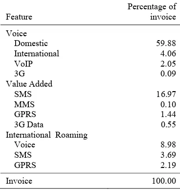
Table 2 Invoice usage of sample by feature
Feature Percentage of invoice Voice Domestic 59.88 International 4.06 VoIP 2.05 3G 0.09 Value Added SMS 16.97 MMS 0.10 GPRS 1.44
3G Data 0.55
International Roaming
Voice 8.98 SMS 3.69 GPRS 2.19
Invoice 100.00
The largest part of invoice were spent for using voice domestic, SMS and voice
international roaming. Subscribers spent over 85% of invoice for using those three features. On the contrary, subscribers spent less than 1% of invoice for enjoying features with 3G. Table 2 displays invoice usage of sample by features.
Segments and Profiles
Because variable tenure and invoice were on different scale, at the first, the data have
been standardized into z values which had
zero mean and standard deviation one, follow
formula z=(x−x)/s where x and s were
mean and standard deviation of samples. Since the Pearson correlation between tenure and invoice was about 0.27, Euclidean
distance was used when executing K-means
clustering algorithms because there is no strong correlation between variables. The number of segments to be indentified was determined in business expert. In this case, Indosat decided to have five segments (Subekti 2009, personal communication).
Figure 1 Plot of tenure vs. invoice by segment
Table 3 Evaluation of segmentation result
Segment RMS
Dist. to Nearest Segment
Dist. Ratio
A 0.30 1.10 3.65
B 0.39 1.10 2.80
C 0.45 1.76 3.89
D 0.91 2.27 2.48
E 1.72 4.88 2.83
Figure 1 shows that K-means allocated
each subscriber into non-overlapping segment, so that one subscriber was exactly in one segment. The root mean square standard deviation for each segment is shown in second column of Table 3. The distance to nearest segment provides a measure of the separation between centroids. Distance ratio was calculated by dividing distance to the nearest segment with the root mean square standard
deviation, RMS. Following the Table 3,
Tenure (month)
6
segment D and E have very large variation within segment, and the segment E was the largest variation. This situation also was shown in Figure 1 obviously. However, the distance ratio were large enough, hence this situation provided the satisfactory result. For further consideration, Appendix 3.A and 3.B
provides more information about K-means
clustering result.
Recall Figure 1, all five segments formed homogenous subscribers within segment, and each segment was also most likely different to each others. The first three segments (A, B, and C) had the lowest invoice, but they were separated by tenure. The last two segments (D and E) had higher invoices compared to A, B, and C. The tenure of segment D and E scatterly distributed or they have very large range.
Table 4 Segment summary information
Segment Subsc. Mean Tenure (Month) Invoice (Rupiah)
A 12,418 15.33 73,865
B 12,562 59.97 137,674
C 4,064 132.63 200,978
D 1,965 69.43 767,615
E 271 92.00 2,123,224
ALL 31,280 52.56 177,341
Profiling was created by exploring size and mean of tenure and invoice of each segment. Those profiles were displayed in
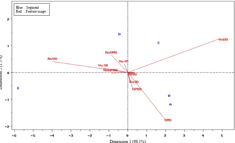
Table 4. In additional, profiling was also created based on percentage of invoice for using features. Information about feature usage were summarized in Appendix 4 and visualized by biplot in Figure 2. Using SAS macro which has been written by Friendly
(1998), the biplot selected α=½ and was able
to cover the information about 99.6%.
Finally, according to Table 4 and Figure 2, the characteristics of segment are described as the following:
1. Segment A :
Segment A was occupied by 39.7% of subscribers. In this case, the new subscribers with the lowest invoice were considered belong to this segment. The largest parts of invoice were spent for utilizing domestic voice and SMS features. Interestingly, the segment A used secondary features, such as voice 3G, GPRS, MMS and data 3G, more than the other segments did.
2. Segment B :
Segment B was occupied by 40.2% of subscribers. It was likely the largest segment. In the average, subscribers of the segment B have registered their subscription since five years. However, they spent the small amount of invoice. The largest parts of invoice of this segment were for voice domestic dialing and SMSs.
Figure 2 Biplot for segment and feature usage
Dimension 1 (98.1%)
Di men sio n 2 (1. 5 % )
7
3. Segment C :
Segment C was only occupied by 13.0% of subscribers. Although the subscribers of this segment contributed low invoice, they were considered had high level of loyalty which indicated by tenures were over 10 years. Subscribers within segment C associated with voice domestic feature.
4. Segment D :
Segment D was only occupied by 6.3% of subscribers. The invoice mean of subscribers within segment D was greater than over-all subscribers did. Additionally, the variance of tenure was very large. It is indicated that this segment include very low tenure and very high tenure. Compared to other segments, subscribers of segment D were VoIP’s users. They also spent invoice more than that of the first three segments in using feature for international connection purposes, such as international voice and roaming.
5. Segment E :
Segment E was only occupied by 0.9% of subscribers. It was the smallest segment formed. The subscribers of segment E were considered as the most profitable which indicated by very high of invoice. Like segment D, the variance of tenure was very large. The most of invoices are allocated for using international features, e.g. international roaming and voice dialing
According to the biplot, segment A had similar behavior with segment B in spending invoice. They were dominated by basic feature users. They also spent their invoice for using several secondary features although in small amount. Hence, segment C had similar behavior with segment D in spending invoice. Segment E was very different to other segments in spending invoice. They were subscribers who need international connectivity services.
The biplot in Figure 2 also provides important information about features usage. According to the biplot, SMS usage and voice domestic were uncorrelated. There were positive correlation between SMS, GPRS, data 3G, MMS and voice 3G usage, but those had negative correlation to SMS international roaming and VoIP usage. Voice international roaming also had positive correlation to voice international and GPRS international roaming usage, but those had negative correlation to voice domestic usage.
Churn Analysis
Model of Churn
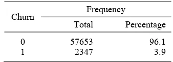
Logistic regression model was used to analyze the churn of subscribers. The explanatory variables were categories of tenure and invoice in three months ago. Those two-explanatory variables were fitted to the active status in current month; ‘churn’ (churn=1) or ‘stay’ (churn=0). It was involved MSISDNs of 60,000 selected randomly. Description of samples provided in Table 5, and for additional information, Appendix 6.A and 6.B provides distribution of sample by categories of tenure and invoice.
Table 5 Description of sample for churn analysis
Churn Frequency
Total Percentage
0 57653 96.1
1 2347 3.9
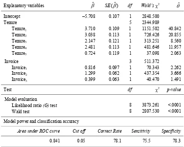
Summary of logistic regression analysis of churn are presented in the Table 6.
Overall model evaluation is examined by
using likelihood ratio or G test. This test
yielded that the logistic model of churn was significant, hence it was effective to estimate churn event based on tenure and invoice in three months ago.
Model performance was measured by area
under ROC curve or C-statistic. In this model,
C-statistic exceeded 0.841. This means that for 84% of all possible pairs of subscribers– one was churn and the other stay–the model correctly assigned a higher probability to those who were churn. It was considered excellent discrimination of churn and stay. For further information, Appendix 7.A provides figure of ROC curve for model of churn.
To assess accuracy of model, an optional cut off point should be decided as that maximizes sensitivity and specificity. In this case, optimal cut off point was at 0.05 (Appendix 7.B) which yielded correct classification rate 78%, sensitivity 76%, and specificity 78%. This result also suggested that model gave satisfactory result in predicting the churn events.
Probability of churn for any given tenure and invoice could be simply illustrated as following. A subscriber with tenure=1 (less than 3 months) and invoice=1 (less than Rp 25,000) has estimated probability of churn:
8
Table 6 Summary of logistic regression analysis of churn
Explanatory variables β) SE(β)) df Wald’sχ2 θ)
Intercept –5.708 0.107 1 2848.500
Tenure 5 2344.989
Tenure1 3.710 0.109 1 1151.502 40.842
Tenure2 3.038 0.113 1 726.426 20.855
Tenure3 2.147 0.121 1 313.251 8.560
Tenure4 2.481 0.113 1 481.646 11.957
Tenure5 0.724 0.119 1 37.098 2.063
Invoice 3 511.372
Invoice1 0.816 0.097 1 70.343 2.262
Invoice2 1.299 0.062 1 437.354 3.666
Invoice3 0.399 0.063 1 40.470 1.491
Test df χ2 p-value
Model evaluation
Likelihood ratio (G) test 8 3873.261 <.0001
Wald test 8 2807.530 <.0001
Model power and classification accuracy
Area under ROC curve Cut off Correct Rate Sensitivity Specificity
0.841 0.05 78.1 75.5 78.3
Subscripts denote categories of explanatory variables.
Using similar calculation, a subscriber with tenure=2 and invoice=1 has estimated probability 0.135. Estimated probabilities of churn for all possible tenure categories and given invoice categories were plotted in the figure of Appendix 8.A. Estimated probabilities of churn for all possible invoice categories and given tenure categories were plotted in the figure of Appendix 8.B.
According to Appendix 8.A, for constant invoice (category 1), estimated probability of churn was decreasing while tenure category was increasing, but estimated probability of churn when tenure=4 was a little more than that of tenure=3. Obviously, tenure=1 had the highest estimated probability of churn, and tenure=6 had the lowest. According to Appendix 8.B, for any given tenure (categories=1), estimated probability of churn was the highest when invoice=2, and reached the lowest when invoice=4.
The last column of Table 6 provided estimated odds ratio which could be interpreted as ratio of odds to experience churn between any given category of explanatory variables and its reference factor. In this research, reference factors were the highest category of each explanatory variable (dummy variables matrix was provided in Appendix 5). To illustrate, odd ratio of
Tenure1=40.842 means the odds of a
subscriber who had tenure at category 1 (less than 3 months) being churn were about
exp(3.710)≈40.842 times greater than the odds
for a subscriber who had tenure at category 6 (more than 60 months). Using similar way, the
odd ratio of Invoice1=2.262 could be
interpreted as the odds of a subscriber who had invoice at category 1 (less than Rp 25,000)
being churn were about exp(0.816)≈2.262
times greater than the odds for a subscriber who had invoice at category 4 (more than Rp 150,000); etc.
Thereby, according to estimated probability and odd ratio, for a given invoice category, provider have to focus more on subscribers who have tenure at category 1, 2 and 4 to avoid them from churning. Furthermore for a given tenure category, provider have to focus more on subscribers who had invoice at category 1 and 2 to avoid them from churning.
Model of ‘At Risk’
Since logistic regression model of churn yielded satisfactory result, subscriber could be
classified into ‘at risk’ or ‘at safe’ group. It
9
model of churn as determined before. If estimated probability of churn was greater than or equal cut off point (0.05) then subscribers were classified as subscriber ‘at
risk’ (risk=1), otherwise as subscriber ‘at safe’
(risk=0). By this approach, about 2.8% of active MSISDNs were categorized as shown in Table 7, and distributions of samples were provided in Appendix 9.A and 9.B.
Table 7 Description of sample for ‘at risk’ analysis
Risk
Frequency
Total Percentage
0 22691 81
1 5387 19
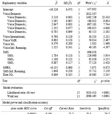
Model of ‘at risk’ was also predicted by logistic regression. In this case, explanatory variables were features usage. Base on stepwise variables selection procedure, there
were nine explanatory variables remain. Those-nine explanatory variables were voice domestic, voice international, voice VoIP, voice 3G, voice international roaming, SMS, GPRS, SMS international roaming, and data 3G usage. MMS and GPRS international roaming usage were removed (Table 8).
The G test yielded that the logistic model
of at risk was significant; hence it was effective to recognize subscribers ‘at risk’ or at safe group based on features usage.
The ROC curve (Appendix 10.A) which
yielded C-statistic of 0.809 suggested that
model is satisfied. This means that for more than 80% of all possible pairs of subscribers – one was categorized as ‘at risk’ and the other categorized as ‘at safe’– the model correctly assigned a higher probability to those who were categorized as ‘at risk’. It was considered excellent classification.
Table 8 Summary of logistic regression analysis of ‘at risk’
Explanatory variables β) SE(β)) df Wald’sχ2 θ)
Intercept –10.126 0.473 1 457.632
Voice Domestic 5 2022.337
Voice Domestic1 3.110 0.083 1 1402.526 22.418
Voice Domestic2 2.265 0.095 1 568.013 9.634
Voice Domestic3 2.047 0.083 1 607.101 7.744
Voice Domestic4 1.535 0.077 1 398.055 4.640
Voice Domestic5 0.785 0.099 1 63.515 2.192
Voice International1 0.798 0.129 1 38.323 2.221
Voice VoIP1 0.903 0.128 1 50.014 2.467
Voice 3G1 0.379 0.280 1 1.832 1.460
Voice Intl. Roaming1 1.525 0.241 1 40.105 4.597
SMS 3 606.858
SMS1 1.784 0.118 1 226.900 5.954
SMS2 1.180 0.123 1 92.856 3.255
SMS3 0.887 0.117 1 57.123 2.428
GPRS1 –0.135 0.060 1 5.071 0.873
SMS Intl. Roaming1 1.640 0.220 1 55.711 5.159
Data 3G1 0.809 0.185 1 19.065 2.245
Test df χ2 p-value
Model evaluation
Likelihood ratio (G) test 15 5833.413 <.0001
Wald test 15 3968.465 <.0001
Model power and classification accuracy
Area under ROC curve Cut off Correct Rate Sensitivity Specificity
0.80924 0.180 71.7 75.8 70.7
10
Accuracy of model was also measured by classification table. According to plot of sensitivity and specificity versus all possible cut off point (Appendix 10.B), an optimal cut off point was preferred to set at 0.180 which led model to had 72% of correct classification rate, 76% off sensitivity, and 71% of specificity. This result also suggested that model was satisfactory to classify subscribers into ‘at risk’ or ‘at safe’ group.
Probability to classified ‘at risk’ for a given category of explanatory variables could be illustrated as following. A subscriber with voice domestic=1 (less than Rp 5,000) and other explanatory variables’ category=1, has estimated probability to classified at risk :
0.665 ) 809 . 0 ... 110 . 3 126 . 10 exp( 1 ) 809 . 0 ... 110 . 3 126 . 10 exp( ≈ + + + − + + + + −
Using similar calculation, a subscriber with voice domestic=2 and other explanatory variables’ category=1 has estimated probability to classified ‘at risk’ 0.461 and a subscriber with SMS=2 and other explanatory variables’ category=1 has estimated classified ‘at risk’ probability 0.521. Estimated probabilities to classified ‘at risk’ for all possible voice domestic categories and given other explanatory variables were plotted in the figure of Appendix 11.A. Estimated probabilities to classified ‘at risk’ for all possible SMS categories and given other explanatory variables were plotted in the figure of Appendix 11.B. Probability to classified ‘at risk’ was decreasing if either category of voice domestic or category of SMS was increasing. Using similar examination, several explanatory variables, except GPRS, had similar tendencies. If other explanatory variables’ category=1 and GPRS category=2 probability of a subscribers to classified at risk equal to 0.695. Its tendency was also reported by negative estimated parameter hence less than zero odds ratio.
Odd ratio of Voice Domestic1=22.418
means the odds of a subscriber who spent less than Rp 5,000 for using voice domestic feature would be classified ‘at risk’ were about 22.418 times greater than the odds for a subscriber who spent more than Rp 150,000
for using same feature. Odd ratio of SMS1
=5.954 means the odds of a subscriber who spent less than Rp 5,000 for using SMS feature would be classified ‘at risk’ were about 5.954 times greater than the odds for a subscriber who spent more than Rp 100,000
for using same feature. Odd ratio of SMS Intl.
Roaming1=5.159 mean the odds of a
subscriber who spent less than Rp 5,000 for
using SMS international roaming feature would be classified ‘at risk’ were about 5.159 times greater than the odds for a subscriber who spent more than Rp 5,000 for using same
feature. Then, odd ratio of GPRS1=0.873
mean the odds of a subscriber who spent less than Rp 5,000 for using GPRS feature would be classified ‘at risk’ were lower about 0.873 times than the odds for a subscriber who spent more than Rp 5,000 using same feature.
CONCLUSION
K–means clustering algorithm was enable
to classify subscribers based on values represented by tenure and invoice. All five segments (A–E) formed homogenous subscribers within segment, and segments were also most likely different to each others. Segment A, B and C had low invoice, but those were separated by tenure. Whereas, segment D and E had higher invoice compared to A, B and C. The tenure of segment D and E scatterly distributed or they have very large range.
Logistic regression model of churn base on invoice and tenure was effective to predict churn event. If invoice was constant, category –one of tenure had the highest estimated probability of churn. Then, if tenure was constant, category–two of invoice had the highest estimated probability of churn. Logistic regression model of ‘at risk’ base on features usage was enable to classify subscribers into ‘at risk’ group or ‘at safe’ group. Voice domestic, voice international, voice VoIP, voice 3G, voice international roaming, SMS, SMS international roaming, and data 3G usage had similar tendency of estimated probability to classified ‘at risk’. The estimated probabilities were decreasing as category of explanatory variables of interest was increasing while the others were constant. In contrast, estimated probability to classified ‘at risk’ was increasing as GPRS usage was increasing.
RECOMMENDATION
Performing segmentation with others
clustering algorithm, such as K-median, Fuzzy
C-Means, etc is highly recommended. If data
11
More detail data of each subscriber in billing, demographic and behavior will yield more accurate prediction of model of churn. Model also will be better if research accommodate trends of subscriber behavior over the time and weighted variables. Other statistical and data mining tools, such as discriminant analysis, survival analysis, decision tree, or a more complex algorithm named artificial neural network are several alternatives to build model of churn.
REFERENCE
Agresti, A. 2007. An Introduction to
Categorical Data Analysis. Second
edition. New Jersey : John Wiley & Sons.
Berry, M.J.A. & G.S. Linoff. 2004. Data
Mining Techniques for Marketing, Sales, and Customer Relationship Management. Second Edition. Indianapolis : John Wiley & Sons.
Bounsaythip, C. & E.R. Runsala. 2001. Overview of data mining for customer
behavior modeling. Research report
TTE1-2001-18. VTT Information
Technology.
Friendly, M. 1998. Construct a biplot of observations and variables uses IML. Version 1.6. http://www.geocities.com /bagusco4/mybook/9.html. [August 31, 2009]
Hosmer, D.W. & S. Lemeshow. 2000. Applied
Logistic Regression. Second edition. Canada : John Wiley & Sons.
Jansen, S.M.H. 2007. Customer segmentation
and customer profiling for a mobile
telecommunications company based on usage behavior : a Vodafone case study. [Master Thesis]. Department of Mathematics of Maastricht University. Limburg.
Johnson, R.A & D.W. Wichern. 1998. Applied
Multivariate Statistical Analysis. Fourth edition. London : Prentice - Hall International.
Lin, Q. 2007. Mobile clustering analysis based
on call detail records. Communications of
the IIMA Vol. 7 Issue 4.
Lipkovich, I & E.P. Smith. 2002. Biplot and singular value decomposition macros for
Excel©. Journal of Statistical Software.
Vol. 7, Issue 5, Jun 2002. Available on http : //www.jstatsoft.org/v07/i05/paper. [August 31, 2009]
MacQueen, J.B. 1967. Some methods for classification and analysis of multivariate
observations. Proceedings of the Fifth
Berkeley Symposium on Mathematical Statistics and Probability. 1. Berkeley, CA : University of California. pp 281 - 297.
Mozer, M.C. et al. 2000. Predicting
subscribers dissatisfaction and improving retention in the wireless
telecommunication industry. IEEE
Transactions on Neural Network, Special Issue on Data Mining and Knowledge Representation.
Mutanen, T. 2006. Customer churn analysis :
a case study. Research report No
VVT-R-01184-06, March 15. VTT Information Technology.
Peng, C.Y.J, K.L. Lee & G.M. Ingersoll. 2002. An introduction to logistic
regression analysis and reporting. The
Journal of Educational Research Vol. 96(1).
Sartono, B et al. 2003. Modul Teori Analisis
Peubah Ganda. Eds. B. Susetyo et al. Bogor : Departemen Statististika IPB. SAS Institute Inc. 2003. SAS User Guide.
Cary : NC.
13
Appendix 1 Description of variables for analysis
Feature Description
MSISDN Mobile subscriber’s ISDN, or commonly called mobile telephone
number.
Tenure Duration of subscription, calculate in day unit.
Invoice Average of invoice in three months (segmentation) or invoice per
month (churn). Invoice is sum of following variable.
Voice
VoDO Invoice for domestic voice, included local and long distance dialing.
VoIN Invoice for international voice.
VoIP Invoice for Voice over Internet Protocol (VoIP).
Vo3G Invoice for voice 3G, i.e. 3G video call.
Value Added Service
SMS Invoice for sending short text message.
MMS Invoice for sending multimedia message.
GPRS Invoice for accessing or browsing internet via GPRS network.
Da3G Invoice for accessing data or browsing internet via 3G network.
International Roaming
RoVO Interconnection fee when dialing to or from foreign countries.
RoSMS Interconnection fee when sending SMS to or from foreign countries.
14
Appendix 2.A Histogram of tenure on standardized data
Appendix 2.B Histogram of invoice on standardized data
Z value of tenure
Z value of invoice
Percent
15
Appendix 3.A Segment summary
Segment
% of
Subscribers RMS
Maximum Distance from Seed to Observation
Nearest Segment
Distance Between Segment
A 39.70 0.3007 1.7411 B 1.0983
B 40.16 0.3917 1.4402 A 1.0983
C 12.99 0.453 1.7968 B 1.7629
D 6.28 0.9116 2.8774 B 2.2662
E 0.87 1.7231 6.6637 D 4.8826
Appendix 3.B Mean and standard deviation of invoice and tenure by segment on standardized data
Segment
Z-value of Invoice Z-value of Tenure
Mean Standard Deviation Mean Standard Deviation
A -0.370384 0.3306458 -0.8959 0.2673418
B -0.141986 0.3939036 0.1784 0.3894284
C 0.084605 0.5580102 1.9267 0.3146814
D 2.112819 0.8808986 0.4057 0.9412675
16
Appendix 4 Percentage of invoice by feature and segment
Feature
Percentage of Invoice
A B C D E
VoDO Voice Domestic 66.26 66.69 66.67 56.49 28.48
VoIN Voice International 1.93 1.67 3.55 5.21 12.38
VoIP Voice VoIP 1.64 1.23 1.70 3.09 2.95
Vo3G Voice 3G 0.22 0.10 0.04 0.05 0.02
SMS SMS 21.60 22.36 17.55 11.99 5.58
MMS MMS 0.14 0.12 0.09 0.08 0.02
GPRS GPRS 2.88 2.14 0.78 0.62 0.12
Da3G Data 3G 2.35 0.00 0.00 0.60 0.00
RoVO Voice Intl. Roaming 1.22 2.75 5.65 13.06 34.15
RoSMS SMS Intl. Roaming 0.80 2.30 3.28 5.36 8.67
17
Appendix 5 Definition of categorical and dummy variables for churn and ‘at risk’ analysis
Predictor Category Value1) Dummy Variables
Tenure 1 0 - 3 1 0 0 0 0
2 3 - 6 0 1 0 0 0
3 6 - 12 0 0 1 0 0
4 12 - 24 0 0 0 1 0
5 24 - 60 0 0 0 0 1
6 > 60 0 0 0 0 0
Invoice 1 0 - 25 1 0 0
2 25 - 50 0 1 0
3 50 - 150 0 0 1
4 > 150 0 0 0
Voice Domestic 1 0 - 5 1 0 0 0 0
2 5 - 10 0 1 0 0 0
3 10 - 25 0 0 1 0 0
4 25 - 100 0 0 0 1 0
5 100 - 150 0 0 0 0 1
6 > 150 0 0 0 0 0
Voice International 1 0 - 5 1
2 > 5 0
Voice VoIP 1 0 - 5 1
2 > 5 0
Voice 3G 1 0 - 5 1
2 > 5 0
Voice International Roaming 1 0 - 5 1
2 > 5 0
SMS 1 0 - 5 1 0 0
2 5 - 10 0 1 0
3 10 - 100 0 0 1
4 > 100 0 0 0
MMS 1 0 - 5 1
2 > 5 0
GPRS 1 0 - 5 1
2 > 5 0
SMS International Roaming 1 0 - 5 1
2 > 5 0
GPRS International Roaming 1 0 - 5 1
2 > 5 0
Data 3G 1 0 - 5 1
2 > 5 0
18
Appendix 6.A Bar chart of subscriber churn and stay by tenure
19
Appendix 7.A ROC curve for model of churn
Appendix 7.B Plot of sensitivity and specificity versus all possible cut off points in the model of churn
Cut off point
Sens
it
ivi
ty
an
d
s
p
ecifi
20
Appendix 8.A Probability of churn by all possible categories of tenure
* Invoice was constant at category 1
Appendix 8.B Probability of churn by all possible categories of invoice
* Tenure was constant at category 1 Category of invoice
Prob
abil
ity
o
f chu
rn
Category of tenure
Prob
abil
ity
o
f chu
21
Appendix 9.A Bar chart of subscriber ‘at risk’ and ‘at safe’ by tenure and invoice
Tenure Invoice
Appendix 9.B Bar chart of subscriber ‘at risk’ and ‘at safe’ by features usage
22
Appendix 9.B
Voice International Usage VoIP Usage Voice International Roaming
Usage
Voice 3G Usage Data 3G Usage GPRS International Roaming
Usage
SMS International Roaming Usage
GPRS Usage MMS Usage
23
Appendix 10.A ROC curve for model of ‘at risk’
Appendix 10.B Plot of sensitivity and specificity versus all possible cut off points in the model of ‘at risk’
Cut off point
Sens
it
ivi
ty
an
d
s
p
ecifi
24
Appendix 11.A Probability to categorized at risk by all possible categories of voice domestic usage
* The other variables were constant at category 1
Appendix 11.B Probability to categorized at risk by all possible categories of SMS usage
* The other variables were constant at category 1 Category of SMS usage
Prob
abil
ity
o
f ‘at
ri
sk’
Category of voice domestic usage
Prob
abil
ity
o
f ‘at
ri