CHAPTER IV
FINDING AND DISCUSSION
A. The Data
A.1 Description of Data
The data were obtained from the result of the listening comprehension test in pre test and post test. There were 53 students from two classes. Both Experimental and control group were given multiple choice in pre test in order to know the students’ prior score in listening comprehension narrative text. The test was calculated based on the indicators in rubrics assessment. From the result of the pre test, it was known that students’ listening comprehension ability was low.
After the pre test had been carried out, the treatment was given to the control group. The control group was taught using audio and the experimental group was taught audio - visual. The result of pre test and post test both groups.
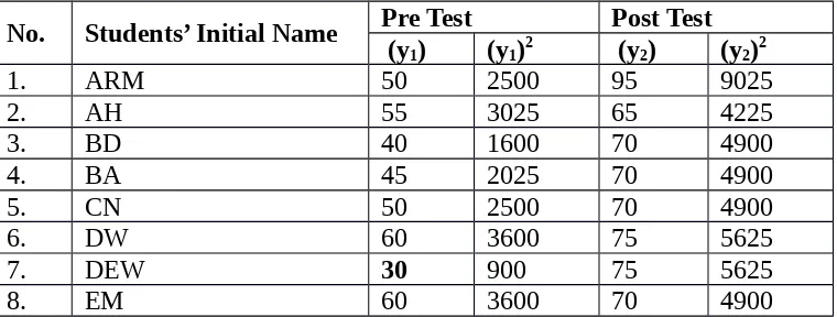
Table 2.1
The Students’ Score of Control Group
No. Students’ Initial Name Pre Test Post Test (y1) (y1)2 (y2) (y2)2
1. ARM 50 2500 95 9025
2. AH 55 3025 65 4225
3. BD 40 1600 70 4900
4. BA 45 2025 70 4900
5. CN 50 2500 70 4900
6. DW 60 3600 75 5625
7. DEW 30 900 75 5625
9. FS 55 3025 80 6400
10. IY 45 2025 95 9025
11. JF 40 1600 90 8100
12. KU 45 2025 90 8100
13. LM 30 900 80 6400
14. MAK 40 1600 85 7225
15. MF 50 2500 80 6400
16. MRD 50 2500 75 5625
17. MY 55 3025 80 6400
18. MYS 40 1600 85 7225
19. NS 40 1600 75 5625
20. NH 45 2025 70 4900
21. NK 35 1225 75 5625
22. NR 60 3600 85 7225
23. PA 60 3600 70 4900
24. SSM 50 2500 65 4225
25. SS 50 2500 65 4225
26. SP 45 2025 65 4225
27. ZW 30 900 95 9025
Total 1255 60525 2095 164975
Mean 46,48 77,59
From the table 2.1 above, it can be seen the control group the total score of pre test is 1255, the lowest score of pre test is 30 and the highest is 60. After fiving treatments, the students have higher score with the total score of post test is 2095, the lowest score for the post test is 65 and the highest is 95.
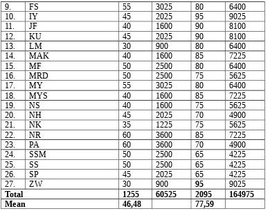
Table 2.2
The Students’ Score of Experimental Group
No. Name Pre Test Post Test
(x1) (x1)2 (x2) (x2)2
1. AHT 45 2025 80 6400
2. AHAR 45 2025 65 4225
3. ARS 50 2500 70 4900
5. DM 45 2025 75 5625
6. DPA 60 3600 80 6400
7. FF 65 4225 85 7225
8. HA 55 3025 80 6400
9. IFN 30 900 90 8100
10. IA 30 900 75 5625
11. LAS 35 1225 90 8100
12. MA 40 1600 80 6400
13. MI 45 2025 85 7225
15. MRH 55 3025 90 8100
14. MS 50 2500 90 8100
16. NA 50 2500 85 7225
17. NRN 45 2025 75 5625
18. OIM 35 1225 65 4225
19. PSR 40 1600 90 8100
20. RS 60 3600 90 8100
21. RAH 60 3600 95 9025
23. SS 40 1600 95 9025
24. SDC 65 4225 95 9025
22. SE 65 4225 95 9025
25. TAP 65 4225 95 9025
26. YAM 40 1600 80 6400
Total Mean
1265 64525 2150 180350
48,65 82,69
From the table 2.2 above, it can be seen the Experimental group the total score of pre test is 1265, the lowest score of pre test is 30 and the highest is 65. After fiving treatments, the students have higher score with the total score of post test is 2150, the lowest score for the post test is 65 and the highest is 95.
From the data, there was a significant difference between the students’ score. It can be seen that the student who were taught by audio - visual got higher score than were taught using audio.
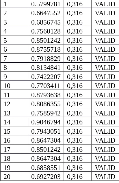
B.1 The Validity
The writer counts the validity of the rest questions by using Audio – Visual. The result can be seen in the following table:
Table 2.3
The Validity of Question
Post Test Experimental Class
1 0.5799781 0,316 VALID
2 0.6647552 0,316 VALID
3 0.6856745 0,316 VALID
4 0.7560128 0,316 VALID
5 0.8501242 0,316 VALID
6 0.8755718 0,316 VALID
7 0.7918829 0,316 VALID
8 0.8134841 0,316 VALID
9 0.7422207 0,316 VALID
10 0.7703411 0,316 VALID 11 0.8793638 0,316 VALID 12 0.8086355 0,316 VALID 13 0.7585942 0,316 VALID 14 0.9046794 0,316 VALID 15 0.7943051 0,316 VALID 16 0.8647304 0,316 VALID 17 0.8501242 0,316 VALID 18 0.8647304 0,316 VALID 19 0.6858551 0,316 VALID 20 0.6927203 0,316 VALID
B.2. Calculation of the Average Value and Standard Deviation
From tabulating the values obtained:
n = 27 So the average is:
X=
∑
Xn =
1255
27 =46,48 And the standard deviation is:
S=
√
n∑
Xi2−
(
∑
Xi)
2n (n−1) =
√
27(60525)−(1255)2
27(27−1)
=
=
= 9,17 S2 = 84,0
2. Calculation of Post-test Data Control Class
From tabulating the values obtained:
n = 27 So the average is:
X=
∑
Xn =
2095
27 =77,59 And the standard deviation is:
S=
√
n
∑
Xi2−
(
∑
Xi)
2n (n−1) =
√
27(164975)−(2095)2
27(27−1)
=
=
= 9,64
∑
X
i2=
60525
∑
X
i=
1255
√
1634175
−
1575025
27
(
26
)
√
59150
702
∑
X
i2=
164975
∑
X
i2=
2095
√
4454325
−
4389025
27
(
26
)
S2 = 92,9
3. Calculation of Pre-test Data Experimental Class
From tabulating the values obtained:
n = 26 So the average is:
X=
∑
Xn =
1265
26 =48,65 And the standard deviation is:
S=
√
n∑
Xi2−
(
∑
Xi)
2n (n−1) =
√
26(64525)−(1265)2
26(26−1)
=
=
= 10,9 S2 = 118,8
4. Calculation of Post-test Data Experimental Class From tabulating the values obtained:
n = 26 So the average is:
X=
∑
Xn =
2150
26 =82,69 And the standard deviation is:
S=
√
n
∑
Xi2−
(
∑
Xi)
2n (n−1) =
√
26(180350)−(2150)2
26(26−1)
=
=
∑
X
i2=
64525
∑
X
i=
1265
√
1677650
−
1600225
26
(
25
)
√
77425
650
∑
X
i2=
180350
∑
X
i2=
2150
√
4689100
−
4622500
26
(
25
)
= 10,1 S2 = 102,0
B.3 Analysis Requirement Test
B.3.1 The Calculation of Normality Test
a. Normality Test of Experimental Class
1. Normality test of Pre-test
Find Z score by using by using the formula:
Zi=
xi− ´x S
1. Zi = 30
−48,65
10,9 = -1,7110
2. Zi = 35−10,948,65 = -1,2523
3. Zi = 40−48,65
10,9 = -0,7936
4. Zi = 45−48,65
10,9 = -0,3349
5. Zi =
50−48,65
10,9 = -0,1239
Find out S(Zi) we use the formula : S(Zi) = Fcum n
1. S(Zi) = 262 = 0,0769
2. S(Zi) = 4
4. S(Zi) =
13
26 = 0,5000 5. S(Zi) = 1726 = 0,6538
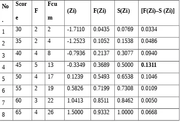
TABLE 3.1
Normality Test of Pre-test at Experimental Group
No .
Scor
e F
Fcu
m (Zi) F(Zi) S(Zi) [F(Zi)–S (Zi)]
1 30 2 2 -1.7110 0.0435 0.0769 0.0334
2 35 2 4 -1.2523 0.1052 0.1538 0.0486
3 40 4 8 -0.7936 0.2137 0.3077 0.0940
4 45 5 13 -0.3349 0.3689 0.5000 0.1311
5 50 4 17 0.1239 0.5493 0.6538 0.1046
6 55 2 19 0.5826 0.7199 0.7308 0.0109
7 60 3 22 1.0413 0.8511 0.8462 0.0050
8 65 4 26 1.5000 0.9332 1.0000 0.0668
From the table above, it can be seen that the Liliefors Observation or L0 =
0,1311 with n = 26 and at real level α = 0, 05 from the list critical value of Liliefors table, Lt = 0,176. It can be concluded that the data distribution was normal,
2. Normality test of Post-test
Find Z score by using by using the formula:
Zi=
xi− ´x S
1. Zi = 65
−83,14
10,2 = 1,7784
2. Zi = 70−83,14
10,2 = 1,2887
3. Zi = 75−83,14
10,2 = 0,7980
4. Zi = 80−83,14
10,2 = 0,3078
5. Zi = 85−83,14
10,2 = 0,1824
Find out S(Zi) we use the formula : S(Zi) = Fcum n
1. S(Zi) = 263 = 0,1112
2. S(Zi) = 264 = 0,1852
3. S(Zi) = 265 = 0,2963
4. S(Zi) = 5
26 = 0,4444
5. S(Zi) = 6
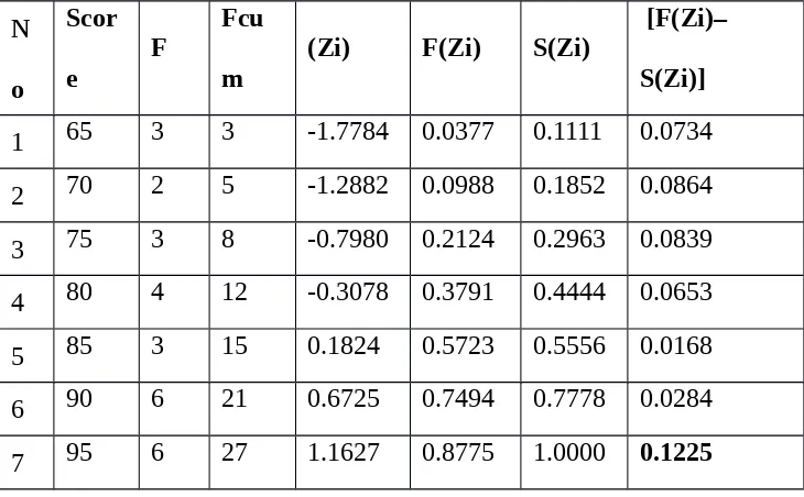
TABLE 3.2
Normality Test of Post-test at Experimental Class
N o
Scor e
F
Fcu m
(Zi) F(Zi) S(Zi)
[F(Zi)– S(Zi)]
1 65 3 3 -1.7784 0.0377 0.1111 0.0734
2 70 2 5 -1.2882 0.0988 0.1852 0.0864
3 75 3 8 -0.7980 0.2124 0.2963 0.0839
4 80 4 12 -0.3078 0.3791 0.4444 0.0653
5 85 3 15 0.1824 0.5723 0.5556 0.0168
6 90 6 21 0.6725 0.7494 0.7778 0.0284
7 95 6 27 1.1627 0.8775 1.0000 0.1225
From the table above, it can be seen that the Liliefors Observation or L0 =
0,1225 with n = 27 and at real level α = 0, 05 from the list critical value of Liliefors table, Lt = 0,176. It can be concluded that the data distribution was normal,
b. Normality Test of Control Class
1. Normality test of Pre-test
Find Z score by using by using the formula:
Zi=
xi− ´x S
1. Zi = 30
−46,48
9,17 = 1,7972 2. Zi = 35−9,1746,48 = 1,2519
3. Zi =
40−46,48
9,17 = 0,7067 4. Zi = 45−9,1746,48 = 0,1614
5. Zi = 50−46,48
9,17 = 0,3839
Find out S(Zi) we use the formula : S(Zi) = Fcum n
1. S(Zi) = 273 = 0, 1111
2. S(Zi) = 1
27 = 0, 1481 3. S(Zi) = 275 = 0, 3333
4. S(Zi) = 275 = 0, 5185
5. S(Zi) =
6
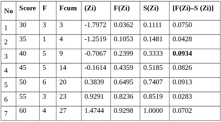
TABLE 3.3
Normality Test of Pre-test at Control Class
No Score F Fcum (Zi) F(Zi) S(Zi) [F(Zi)–S (Zi)]
1 30 3 3 -1.7972 0.0362 0.1111 0.0750
2 35 1 4 -1.2519 0.1053 0.1481 0.0428
3 40 5 9 -0.7067 0.2399 0.3333 0.0934
4 45 5 14 -0.1614 0.4359 0.5185 0.0826
5 50 6 20 0.3839 0.6495 0.7407 0.0913
6 55 3 23 0.9291 0.8236 0.8519 0.0283
7 60 4 27 1.4744 0.9298 1.0000 0.0702
From the table above, it can be seen that the Liliefors Observation or L0 =
0,0934 with n = 27 and at real level α = 0, 05 from the list critical value of Liliefors table, Lt = 0,176. It can be concluded that the data distribution was normal,
2. Normality test of Post-test
Find Z score by using by using the formula:
Zi=
xi− ´x S
1. Zi = 65−76,92
9,17 = 1,2999 2. Zi =
70−76,92
9,17 = 0,7546 3. Zi = 75−9,1776,92 = 0,2094
4. Zi =
80−76,92
9,17 = 0,3359 5. Zi = 85
−76,92
9,17 = 0,8811
Find out S(Zi) we use the formula : S(Zi) = Fcumn
1. S(Zi) = 4
27 = 0,1538
2. S(Zi) = 6
27 = 0,3846
3. S(Zi) =
5
27 = 0,5769
4. S(Zi) = 274 = 0,7308
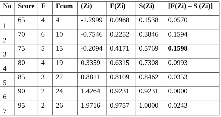
TABLE 3.4
Normality Test of Post-test at Control Class
No Score F Fcum (Zi) F(Zi) S(Zi) [F(Zi) – S (Zi)]
1 65 4 4 -1.2999 0.0968 0.1538 0.0570
2 70 6 10 -0.7546 0.2252 0.3846 0.1594
3 75 5 15 -0.2094 0.4171 0.5769 0.1598
4 80 4 19 0.3359 0.6315 0.7308 0.0993
5 85 3 22 0.8811 0.8109 0.8462 0.0353
6 90 2 24 1.4264 0.9231 0.9231 0.0000
7 95 2 26 1.9716 0.9757 1.0000 0.0243
From the table above, it can be seen that the Liliefors Observation or L0 = 0,
1598 with n = 26 and at real level α = 0, 05 from the list critical value of Liliefors table, Lt = 0,176. It can be concluded that the data distribution was normal, because L0
B.3.2 The Calculation of Homogeneity Test
a. Homogeneity Test of Pre-test
Fh=S1 2
S22
Where : S12 = the biggest variant
S22 = the smallest variant
Based on the variants of both samples of pre-test found that:
Sex2 = 118,1 N = 27
Scont2 = 84,0 N = 26
So:
Fcount =
S2keks S kcont2
Fcoun =
118
,
1
84
,
0
=
1,40
Then the coefficient of Fcount = 1,40 is compared with Ftable, where Ftable is
Because of Fcount< Ft atau (1,40 < 1,95) so it can be concluded that the variant
is homogenous.
b. Homogeneity of Post-test
Fh=S1 2
S22
Where : S12 = the biggest variant
S22 = the smallest variant
Based on the variants of both samples of post-test found that:
S
eks2 = 92,9 N = 26S
kont2 = 102,0 N = 27So:
Fh =
S2keks S kcont2
Fh =
102
,
0
92
,
9
=
1,09
Then the coefficient of Fcount = 1,09 is compared with Ftable, where Ftable is
Because of Fcount< Ft atau (1,09 < 1,95) so it can be concluded that the variant
is homogenous.
C. Hypothesis Testing
The formula of t-test and distribution table of the t-critical values is applied in testing the hypothesis. The testing hypothesis is conducted in order to find out whether the hypothesis is acceptable or rejected. The basic of testing hypothesis is as follows:
t =
Ma−Mb
√
(
∑
da
2+
∑
db
2 Na+Nb−2
)
(
1 Na+
1 Nb
)
The calculation of the t-observed :
Ma = 34,03 Mb = 31,11
∑
da 2 = 0,22∑
db2= 0,03
Na = 25 Nb = 26
t =
Ma−Mb
√
(
∑
da
2+
∑
db
2 Na+Nb−2
)
(
1 Na+
1 Nb
)
=
34,03−31,11
√
(
0,22+0,03 25+26−2)(
1 25+ 1 26
)
= 2,92√
(
0,25 49)
(0,7) = 2,92= 2,92
√
0,35 = 2,920,59 = 4,94
Ha : μ1<μ2, it means that teaching English by using Audio– Visual significantly affect on the students’ ability in listening comprehension. In other words, Ha is accepted if the t-observed ¿ t-table.
After calculating the data, the writer found that t-observed (4,94) was higher than t-table (2, 01) at the level of significance of α=0,05 and at the degree of freedom (df) = Nx + Ny – 2. Where Nx the total numbers of Experimental group is 26
and Ny was the total numbers of control group is 27. Thus, df = 26 + 25 – 2 = 51.
Based on the data, it can be concluded that the students’ ability taught by using Audio – Visual media is higher than taught by using audio only.
D. Research Finding
1. Base on the result of the calculation above, it was found that students’ ability in listening comprehension by using audio – visual got mean score of the pre test in experimental group was 46,48 the lowest score is 30, the highest score is 65. Meanwhile Mean score of the post test in experimental group was 82,62 the lowest score is 65, the highest score is 85.
in control group was 77,59 the lowest score is 65 and the highest score is 95. It can be assumed that the treatments have been done successfully.
3. Based on the statistical computation test was found that the coefficient
t-observation = 4,94. Where the coefficient of ttable 2.01. It is obtained that t-observation ¿ t-table.
It means that there was significant effect of using Audio – Visual in teaching English on the students’ ability in listening comprehension. It was indicated that Ha was
accepted and Ho was rejected.
E Discussion
The media is one factor determining the success of learning. Through audio-visual then the learning process will be more interesting and exciting. Material presented orally by the teacher sometimes not fully understood by the students. Then the media was necessary for the learning process, which is audio-visual to help the learning process in teaching listening comprehension. And as a tool to teaching and learning process that teach the learning material so that the teaching objectives can be achieved with better and more perfect.
Using audio-visual in teaching English can Affect students' ability in listening comprehension, because audiovisual has an element of sound, visual, and gestures. Dale says that (in Arsyad book) using audio-visual in listening teaching is to enable the eyes and ears of students during the learning process. So that the learning process becomes more active1. Because using audio-visual in teaching listening
comprehension students will be more concentration, because they see, hear directly material taught using audio-visual equipment. And audio-visual aid easier for students
to be able to digest the information that was submitted directly. And affirmed by Rudy Breatz (in Arsyad books), audio-visual that can Affect students' ability to improve memory, learning outcomes, and comprehension.2
According to Azhar Arsyad the advantages of using audio-visual:
1. The teaching materials will be quite vague so it can be understood by students, and students can master English language learning objective in listening comprehension.
2. Teaching will be more varied, not only verbal communication through said by the teacher, so that the students not bored and teachers are not run out of steam when teaching.
3. The students more active learning, such as observe, listen, and comprehendand etc.
4. The use of audio-visual teaching will attract more attention so it can motivate students to learn.
5. Can describe an exact process, and can be witnessed repeatedly.
6. Can stimulate active participation of hearing students, as well as to develop imagination like Wring, drawing, etc.3
Kustiyono say that the media is one important component in improving the quality of learning, one of which is an audio-visual.4 Because of with use of
audio-visual teaching materials can facilitate convey. And using audio-audio-visual in teaching
2 Ibid. P. 35 3 Ibid. P. 30
listening can enhance students' understanding, presenting interesting material, and get information.
Djamarah say that (in Arsyad book) use of audio- visual book to improve effectiveness and efficient teaching and learning, so that students are able to develop their thinking. Learning to use double senses of hearing and sight that will provide benefits for the students, because the students will learn more focus.5 This means that
students who learn to use audio-visual in teaching listening comprehension will be more concentration in order to understand the material that has been delivered so that students can answer the questions that the teacher.
Teaching is obtained only in the form of words, it is difficult to be imagined and understood by students. Thus the audio-visual media that help the learning process becomes more effective, because the students directly listen, see, and understand directly the same time. Therefore it can be concluded that by using audio-visual can enhance students' skills in listening comprehension.