Voimakkaiden TMS-artefaktojen analyysi ja poisto EEG-datasta

(1)

Reeta Korhonen

Characterizing and removing strong

TMS-induced artifacts from EEG

Faculty of Electronics, Communications and Automation

Thesis submitted for examination for the degree of Master of Science in Technology.

Espoo 21.4.2010

Thesis supervisor:

Prof. Risto Ilmoniemi Thesis instructor:

Prof. Risto Ilmoniemi

A

’’

Aalto University

School of Science and Technology

(2)

aalto university

school of science and technology

abstract of the master’s thesis

Author: Reeta Korhonen

Title: Characterizing and removing strong TMS-induced artifacts from EEG Date: 21.4.2010 Language: English Number of pages:6+39 Faculty of Information and Natural Sciences

Department of Biomedical Engineering and Computational Science

Professorship: Biomedical engineering Code: Tfy-99 Supervisor: Prof. Risto Ilmoniemi

Instructor: Prof. Risto Ilmoniemi

Transcranial magnetic stimulation (TMS) combined with electroencephalogra-phy (EEG) provides a means to non-invasively stimulate cortical brain areas and to monitor the evoked neuronal activation and connectivity. However, TMS causes various artifacts that can distort the EEG signal. Especially in the lateral areas of the brain, which include the main areas of language pro-cessing, the muscle artifact can mask the neuronal activity for tens of milliseconds. The purpose of this thesis was to characterize the artifacts and find ways to reduce them during data acquisition and in offline analysis. The results show that the artifact is highest in anterior and lateral areas and that the high amplitude and long duration of the artifact in lateral areas makes removing it a challenging task.

Two methods of offline artifact removal were evaluated for the high-artifact data. Independent component analysis (ICA) and multiple-source modeling were able to reduce the artifact, but also affected the brain signal during or after the artifact.

(3)

aalto-yliopisto

teknillinen korkeakoulu

diplomity¨on tiivistelm¨a

Tekij¨a: Reeta Korhonen

Työn nimi: Voimakkaiden TMS-artefaktojen analyysi ja poisto EEG-datasta Päivämäärä: 21.4.2010 Kieli: Englanti Sivumäärä:6+39 Informaatio- ja luonnontieteiden tiedekunta

L¨a¨aketieteellisen tekniikan ja laskennallisen tieteen laitos

Professuuri: Biomedical engineering Koodi: Tfy-99 Valvoja: Prof. Risto Ilmoniemi

Ohjaaja: Prof. Risto Ilmoniemi

Transkraniaalisen magneettistimulaation (TMS) ja elektroenkefalografian (EEG) avulla voidaan stimuloida aivokuorta ei-invasiivisesti ja samalla tarkkailla aiheutetun aivoaktivaation leviämistä. TMS-stimulaatio kuitenkin aiheuttaa EEG-signaaliin artefaktoja, jotka voivat kestää jopa kymmeniä millisekunteja ja kokonaan peittää tutkittavan aivoaktiivisuuden. Lihasten aktivoituminen aiheuttaa artefaktoja erityisesti lateraalisilla aivoalueilla, mm. stimuloitaessa aivojen pääasiallisia kielialueita.

Tämän työn tarkoitus oli määrittää, mistä artefaktat johtuvat, ja kuinka niitä voitaisiin pienentää mittauksen aikana ja sen jälkeisessä data-analyysissä. Arte-faktojen todettiin olevan suurimmillaan stimuloitaessa anteriorisia ja lateraalisia aivoalueita. Näillä alueilla artefaktojen poistoa vaikeuttavat niiden voimakkuus ja pitkä kesto.

Artefaktojen poistoon analyysivaiheessa kokeiltiin kahta menetelmää. Riip-pumattomien komponenttien analyysi (independent component analysis, ICA) ja monilähdemalliin perustuva korjaus pystyivät poistamaan osan häiriöpiikeistä, mutta vaikuttivat myös aivoperäiseen signaaliin artefaktan aikana ja jälkeen.

(4)

Acknowledgements

This thesis was written at the Department of Biomedical Engineering and Computational Science at the Aalto University School of Science and Technology during the years 2009 and 2010. The experimental work was conducted at the BioMag Laboratory in the Helsinki University Central Hospital.

I would like to thank my instructor and supervisor Risto Ilmoniemi for expert guidance and comments on this thesis, as well as on the special assignment completed in 2009. I thank Hanna Mäki for teaching me the secrets of TMS and for advising me in all things I thought to ask, and Jyri Lautala and Anne-Mari Vitikainen for getting me started with this project. Thanks also to Julio César Hernández Pavón for helping me with the measurements and analyses. Special thanks to Johanna Metsomaa and Jukka Sarvas for making the mathematical methods understandable to a biologist. I would also like to thank the helpful staff of BioMag laboratory for their assistance and my fellow students at BECS for lunch company and laughs.

Reeta Korhonen Espoo, April 21, 2010

(5)

List of Abbreviations

ACC Anterior cingulate cortex AF Anterior fasciculus APB Abductor pollicis brevis

DT-MRI Diffusion tensor magnetic resonance imaging EEG Electroencephalography

EMG Electromyography EOG Electro-oculography ERP Event-related potential

fMRI Functional magnetic resonance imaging ICA Independent component analysis LIFG Left inferior frontal gyrus

MEG Magnetoencephalography MEP Motor evoked potential MRI Magnetic resonance imaging MT Motor threshold

MTG Medial temporal gyrus

NBS Navigated brain stimulation PCA Principal component analysis TMS Transcranial magnetic stimulation STG Superior temporal gyrus

(7)

Introduction

This work continues the connectivity study of language-related brain areas, the first part of which is reported in the thesis of Jyri Lautala [1]. Transcranial magnetic stimulation (TMS) is a method for stimulating the superficial parts of the brain through the skull, noninvasively. Combined with electroencephalography (EEG) it can be used to probe cortical excitability and connectivity. However, TMS introduces various artifacts to the EEG recording that can distort and mask the brain activity. The artifact problem of TMS–EEG and some methods of artifact removal are discussed and tested in this thesis.

1.1 Transcranial magnetic stimulation

Transcranial magnetic stimulation (TMS) activates cortical neurons by a magnetic pulse. Depending on the stimulation parameters, it can be used to test cortical excitability, to disrupt or increase brain activity momentarily, or to modulate activity for a longer period. TMS was introduced by Barker et al. in 1985 [2] and has since been used to study the functions of different brain areas and the connections between them and the peripheral nervous system. The primary motor cortex is a popular target for stimulation since the resulting responses, motor evoked potentials (MEPs), measured by recording the electromyogram (EMG) from the target muscles, are easily quantifiable [3]. Other easily identifiable effects include phosphenes, seen by the subject when the primary visual cortex is stimulated, and speech arrest when activity in Broca’s area is disrupted by stimulation [4]. Cortical activity can be directly monitored with electroencephalography (EEG) (see section 1.2) or other functional imaging methods.

The stimulation is achieved by passing current through a coil, which is most commonly circular or eight-shaped. The current creates a magnetic field that penetrates the skull and induces currents in the cortex and the appropriately oriented nearby axons. The wave shape of the current pulse can be monophasic, biphasic or polyphasic, meaning that the current in the coil travels in one or two directions or reverses direction multiple times, respectively. [5]

The mechanism of neuronal activation in magnetic stimulation is still somewhat controversial. In contrast to the long straight axons of the peripheral nervous system, which are excited at the peak of the electric field gradient, the shorter and often curved axons of the cortex are more likely to be excited at end points or bends where the induced current flows out of the axon [6], [7], [3]. According to Nagarajan et al. [8], the role of dendrites and cell bodies in excitation by magnetic stimulation is insignificant due to their small size relative to the field magnitudes, although their

(8)

relatively long time constants should make them easier to excite than axons with shorter time constants [9], [10]. The currents induced by TMS are tangential to the skull, and the axons having at least some part in the same plane are the most likely to be stimulated by these currents. Neurons located on walls of the sulci best fill this requirement, and the most effective stimulation is therefore achieved when the maximal induced current is directed perpendicular to a sulcus towards the center of the gyrus. [5]

1.1 Electroencephalography

Electroencephalography (EEG) is a relatively simple and non-invasive way to measure brain activity. The signal is measured from electrodes attached to the scalp surface and it represents the combined, postsynaptic activity of many neurons. EEG detects most easily radial and to some degree also tangential currents that are flowing in the extracellular space. The contribution of action potentials to the EEG signal seems to be small compared with the postsynaptic events. [11] In comparison to other methods of functional imaging, such as fMRI, EEG has good temporal resolution (in the millisecond range) but relatively poor spatial resolution. As EEG is recorded on the surface of the head, it can detect activity in superficial and to some extent also deeper areas of the brain, and the skull and skin distort the original signal. Because currents may produce potentials that cancel each other out, it is impossible to exactly determine the sources of EEG activity. However, there are many methods for solving the inverse problem to estimate the locations of electric currents that would produce the recorded signal. [12, 13]

Measurement of spontaneous EEG is used in the clinic to, for example, diagnose epilepsy or sleep disorders. Event-related potentials (ERPs), meaning the EEG responses associated with certain actions or external stimuli, can be studied by repeating the action or stimulus and averaging these epochs to eliminate the non-related background activity. This approach can give information about the cortical areas involved in different cognitive tasks and processes. [11] Filtering and Fourier transformation can be utilized to analyze the spectral properties of EEG. Synchronous activity of many neurons in neighboring areas produces spontaneous oscillations, different frequency bands of which are associated with certain processes and cognitive states, such as memory, sleep, or attention (reviewed in [14]). Also the cohesion of the spontaneous oscillations in different brain areas, indicating functional connectivity between the areas, can be analyzed [15].

In addition to the brain activity, EEG also registers eye and muscle movements, which need to be filtered or projected out from the data before the analysis. These artifacts are often much larger in amplitude than the neuronal signal and present on multiple channels. Various methods of artifact removal are presented in the following sections.

(9)

1.1.1 Sources of artifacts in TMS–EEG

The TMS pulse induces currents also in the EEG electrodes, introducing an artifact that may last about 5 ms after the pulse [16]. If no special precautions are taken, the pulse saturates the amplifiers and masks the underlying neural activity foreven hundreds of milliseconds [17]. This problem has been solved by using amplifiers with a much wider range [16] or by a sample-and-hold circuit that cuts the connection between the electrodes and the amplifier for a few milliseconds during and after the pulse [18], enabling the recording of cortical activity as early as 5 ms after the pulse.

Part of the TMS artifact is caused by the polarization of the skin–electrode contact, especially if the impedance of the connection is high. Therefore, the impedance of the electrodes should be made as low as possible, preferably below 5 kΩ. The magnitude of this type of artifact can be further reduced by puncturing the skin under the EEG electrodes to reduce the impedance between electrodes and the skin [19].

In addition to exciting the neurons directly, the magnetic pulse also affects the muscles and motor nerves underneath the coil. Muscle activation and eye movements cause artifacts in the EEG that may mask the actual brain activity. The size of the muscle artifact depends on the stimulation location, with larger artifacts in lateral areas, such as the temporal lobe, close to the jaw muscles, compared with more medial areas, such as the hand representation area in the primary motor cortex. Eye artifacts are caused by eye movements and blinking. The traditional way of dealing with these artifacts has been to instruct the subject to focus on one spot during the whole exam, and rejecting epochs that contain blinks or large artifacts. The TMS pulse can also excite the somatosensory nerve endings and the coil click activates the auditory system of the subject. These activations can be seen in EEG as auditory or, to a lesser extent, somatosensory evoked potentials. [for review, see 17]

1.1.2 Artifact removal from EEG

The simplest ways to reduce the effect of artifacts is to exclude by visual or automatic inspection the epochs that contain artifacts, or, in case of eye movement artifacts, to subtract a signal that is proportional to that in an EOG channel (assumed to equal eye activity) from the EEG channels. The exclusion method still retains some eye artifact in the signal, and the subtraction removes some neuronal signal in addition to the artifact [20], so other, more efficient methods are required, especially when the artifact is tightly coupled to the brain activation under study, as is the case in TMS–EEG.

1.1.2.1 Independent component analysis

Independent component analysis (ICA) is a computational method for extracting independent sources from a data set. In EEG analysis it can be used to identify sources

(10)

in the brain or to separate artifacts from the brain activity. Other applications of ICA include, for example, feature extraction. The fundamental assumption of ICA is that the measured signal in each channel represents a linear combination of the source signals via a mixing matrix. The goal of ICA is, after appropriate data compression, to find the mixing matrix and to use the inverse of that matrix to extract the sources from the recorded data. In EEG analysis, the independent components are thought to correspond to the brain and artifact source signals and the mixed signals are recorded by the electrodes. The mixing matrix determines how the electrodes see each source, and each column of the mixing matrix represents the topography of the corresponding independent component, i.e., the relative voltage measured by each electrode if only that source was active. [21]

The ICA method uses assumptions of the statistical properties of the sources to deduce the mixing matrix. The main assumption is that the source components are statistically independent. The mixed signals and the independent components are treated as random variables and their time signals are considered to represent random samples of the random variables. Another assumption is that (at least all but one of) the independent components have a non-gaussian distribution. The non-gaussianity assumption is important because the identification of the independent components relies on the central limit theorem, according to which the sum of two independent random variables has a more gaussian distribution than either of the two alone. Thus, minimizing gaussianity is the key to finding the mixing matrix and the independent components. The non-gaussianity of the component is measured by a contrast function that may represent kurtosis or skew, or approximates negentropy. The absolute value of kurtosis, measuring the peakedness of the distribution, is a classical method to measure gaussianity but rather sensitive to outliers in the data. Skewness of the distribution measures its asymmetry. Functions approximating negentropy are generalizations of the kurtosis function and the derivatives of these contrast functions include the hyperbolic tangent and a gaussian function. [21]

Independent component analysis has some limitations. The energies and signs of the independent components can not be estimated and the order of the components is random in each run of the algorithm. [21] The maximum number of components that can be separated equals the number of channels, but reducing the dimension of the data by principal component analysis or estimating fewer components can produce better results, especially if the number of samples is low [22]. According to Onton et al. [23], a sufficient amount of samples to evaluate m components, is at least 20m2.

The FastICA software package (version 2.5 [24]) uses a fixed-point algorithm to minimize the contrast function for finding the independent components. The data are

(11)

first preprocessed by centering, data compression, and whitening. [21] This is done by principal component analysis (PCA), which transforms the centered data XC into the

whitened matrix whose rows are the principal eigenvectors of XC·XCT, where T stands

for transpose. The first eigenvector represents as much of the variability in the data as possible, and each component after that contains as much of the remaining variability in the data as possible. [25] At this stage, the dimension of the data can be reduced by leaving out the most insignificant eigenvectors contributing least to the variability in the data. For the FastICA algorithm, the user can choose one of the four contrast functions presented above. Decorrelation is needed to prevent the algorithm from converging to the same result many times. The FastICA program offers two approaches to decorrelation: deflation, where the components are estimated one by one, and the symmetric approach. [21]

As stated above, ICA can be used in EEG or magnetoencephalography (MEG) analysis to separate independent brain and artifact sources. ICA has been shown to be able to separate eye movement artifacts from brain activity [26], [27]. Vigario et al. [28] demonstrated the potential of this technique on MEG data, separating common artifact sources, such as eye movements and muscle activity, from the brain activity. At least in MEG data, ICA can also separate different components of brain activity, tactile response from auditory response, and several components with different latencies from an auditory response (reviewed in [29]). Even the TMS-evoked muscle artifact, although usually larger than other types of artifacts and more tightly coupled temporally to the evoked brain response, has been successfully separated from TMS– EEG data by ICA [30].

1.1.2.2 Multiple source artifact correction method

Some success in removing eye and TMS artifacts has been achieved using a multiple-source approach formulated by Berg and Scherg [20]. Like ICA, also this method presents the EEG activity as the product of two matrices: a lead field matrix, every column of which represents the topography, or the signal distribution of one source to the electrodes, and a source matrix in which every row is the waveform of one source. If the lead field matrix is known, the brain source activities can be extracted from EEG data and the artifact sources can be removed. Litvak et al. [31] used the method of Berg and Scherg in an iterative process to determine the lead field matrix. The lead field matrix for artifact sources is estimated by performing a principal component analysis of a time segment dominated by artifact and taking the first one or a few eigenvectors that represent most of the variability of the signal. At the first stage, when the real brain activity is not yet known, the brain sources are estimated by a surrogate model containing 15 dipoles placed inside the spherical head model. The electric field produced by each source is calculated at the electrode locations, resulting in one

(12)

column of the lead field matrix per one brain source. The lead field matrices of artifact and brain sources are concatenated, the whole matrix is then inverted, and the source waveforms are obtained as the product of the inverse matrix and the original EEG waveforms. The artifact sources are then set to zero and a set of new EEG signals is calculated. From the grand average of this corrected EEG of many subjects, a more accurate model of brain activity is constructed. At the second stage, this new model is used, instead of the surrogate model, to represent brain activity when estimating the lead field matrix. The correction of EEG is then done again for the original data of each subject. In the study of Litvak et al. [31], the procedure was able to remove the TMS-induced artifact spikes from the EEG data.

1.2 Speech processing in the brain

According to the traditional view of language processing in the brain, two cortical areas are responsible for understanding and producing speech. Broca’s area, located in the inferior frontal gyrus of the left hemisphere, was thought to contain the motor representations of words. In contrast, Wernicke’s area, located in the posterior temporal lobe of the left hemisphere, was supposed to contain auditory word representations. In light of several lesion and functional imaging studies, this view has since been challenged and a new, more complex model including separate phonetic, semantic, and grammatical levels is arising. The present view suggests that the various subtasks of language processing are distributed over many cortical areas including sites in the frontal, parietal and temporal cortex. For example: superior temporal lobes bilaterally are needed to extract phonetic features from speech, whereas semantic representations are localized in the left, and possibly to a smaller extent in the right, middle and inferior temporal gyri. (For review, see [32]) Also TMS-studies have contributed to the knowledge of the language areas. For example, a functional division in the left inferior frontal gyrus language areas, semantic and phonological processing localized to the rostral and caudal portions, respectively, was demonstrated using TMS [33]. On a more general network level, a recent theory suggests that a ventral processing stream, involving frontal and temporal regions and connections in both hemispheres, is responsible for speech comprehension, and that a dorsal stream, heavily lateralized to the left hemisphere, maps acoustic signals to articulatory networks in the frontal lobe [34]. In general the role of the left hemisphere seems to be more dominant in most individuals, but bilateral function is still essential for some tasks [32, 33].

Several diffusion tensor magnetic resonance imaging (DT-MRI) studies, which can reveal white-matter connections by tracking the diffusion of water molecules, have shown that the white-matter tract arcuate fasciculus (AF) connects the frontal and temporal areas to each other and to other language-processing areas in the parietal cortex [35, 36]. The tract consists of a long segment connecting Broca’s and

(13)

Wernicke’s areas directly, a posterior segment connecting Wernicke’s area with inferior parietal cortex language area and an anterior segment connecting this with Broca’s area, creating an indirect route between frontal and temporal language areas [35, 37]. AF is one part of a more extensive white-matter tract called the superior longitudinal fascicle, which connects frontal areas to more posterior ones in the same hemisphere [38], and forms the dorsal pathway of the dual-stream model [34, 39]. Besides the convenient anatomical location, the role of AF in language is supported by the observation that it is much more prominent in humans than in nonhuman primates [40] and therefore possibly has an important role in the evolution of language. This anatomical connection between the language areas is stronger in the left hemisphere than in the right [40, 41, 42, 43, 44, 45, 46, 47, 48] although this finding was not significant in all studies [38, 37]. The asymmetry is thought to reflect the functional lateralization of language, although Vernooij et al. [44] report that the leftward anatomical asymmetry exists also in left-handed people who have right-lateralized language functions.

Functional links between the language-related and other areas have been studied with both functional imaging methods and TMS. In a functional MRI (fMRI) study, it was discovered that the activity in the left inferior frontal gyrus (LIFG) predicts activity in the left superior and medial temporal gyri (STG and MTG) and that this connection was modulated by activity in the anterior cingulate cortex (ACC) [49]. EEG and TMS studies have revealed a functional connection between motor areas and the areas responsible for processing words referring to actions performed hands, legs or mouth [50, 51]. The connection between the prefrontal language areas and the motor areas is bidirectional, reading of words activating motor areas related to the meaning of the word [50], and magnetic stimulation of the relevant motor areas facilitating word processing [51].

A previous thesis study [1] attempted to test the functional connectivity between Broca’s and Wernicke’s areas directly by stimulating one area with TMS and monitoring the spreading of activity to other areas by EEG. In comparison to other functional methods that describe brain activity during language-related cognitive tasks, this approach can demonstrate the causal connections of brain activity. The initial activation is targeted to only one area and secondary activations can be assumed to occur in areas connected to the stimulation site. However, due to the lateral location of the language areas, the early responses were masked by large muscle artifacts which prevented tracking of the connectivity. The purpose of this study is to characterize the artifact, find out how it can be avoided, and to explore methods for offline artifact removal from the EEG data.

(14)

2 Methods

2.1 Magnetic stimulation protocols

Nexstim TMS system and eXimia Navigated Brain Stimulation software (version 3.2.1, Nexstim Ltd., Helsinki, Finland), which enables the targeting of the stimulation according to the previously acquired magnetic resonance image (MRI) of the subject, were used to target and deliver the TMS pulses. The biphasic figure-of-eight coil was held manually. A piece of plastic foam was placed between the coil and head to avoid direct contact of the coil and the electrodes and to reduce the transmission of coil vibration. During stimulation, the subject wore earplugs and was asked to relax and rest his or her head on the neck support of a reclining chair, keep eyes open and to focus on a mark on the wall.

Nexstim eXimia EMG system was used in combination with NBS software to measure the motor threshold of each subject from the thumb muscle abductor pollicis brevis (APB). Disposable electrodes were attached to the belly of the muscle, on a bony area near the metacarpophalangeal thumb joint and on the back of the same hand (ground). The representation area of the muscle in the motor cortex was located by stimulating with a relatively high intensity the surrounding area and finding the spot that gave the highest muscle response. This spot was then stimulated and the intensity lowered until only five out of ten stimuli elicited a response over amplitude of 50 µV. This stimulation intensity defined the motor threshold (MT) intensity.

2.1.1 Artifact experiment: Stimulation site

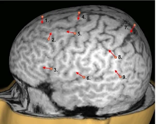
One male subject (subject 1) received stimulation (100% MT) to nine sites on the left hemisphere (Figure 1). The sites were chosen to test the dependence of artifact size on stimulation location in the medial–lateral and anterior–posterior axes, while being close to areas expected to play a role in the study of speech areas. Area 3 is close to Broca’s area and area 9 corresponds roughly to Wernicke’s area [34]. The stimulation direction was chosen according to local anatomy in each site to be approximately perpendicular to the nearest sulcus. 30–50 pulses were delivered to each location at random intervals of 1500–3500 ms.

2.1.2 Artifact experiment: Stimulation intensity

Part of the stimulation intensity experiment was conducted on subject 1. Stimulation was administered to one “high-artifact” site (number 3 in Figure 1) and one “low-artifact” site (number 4 in Figure 1) at 90, 80 and 60% MT. 50 pulses were delivered to each site at each intensity. Data of sites 3 and 4 from the stimulation site experiment were used as the 100% condition in data analysis.

(15)

Figure 1. Stimulation sites 1–9 on subject 1. The arrow indicates the direction of the second phase of the current pulse, which is the most effective phase.

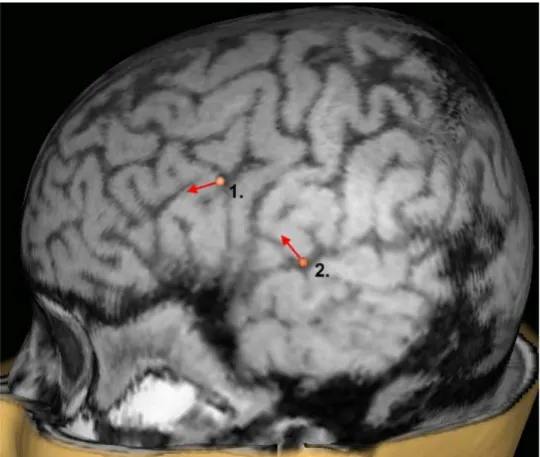
Lower intensities were studied on subject 2 (female). Two sites, corresponding to Broca’s and Wernicke’s areas, were stimulated (Figure 2). 70 stimuli were applied to the two sites with 100, 50, 40, and 30% MT intensity. The data were filtered with a second-order 100-Hz low-pass filter before measuring the artifact.

2.1.3 Artifact experiment: Amplifier gating time

One female subject (subject 3) received three sequences of stimulation on two sites shown in Figure 3. Both sites were laterally located and were expected to give relatively high muscle artifacts. Between sequences, the EEG amplifier gating time (the time the amplifier output is kept constant by a sample-and-hold circuit) was adjusted. Both sites were stimulated with the gating time being 2 (default), 5, and 10 ms. The stimulation intensity was kept at 100% MT; 100 pulses were delivered in each sequence at random intervals of 1500–3500 ms.

(16)

Figure 2. Stimulation sites on subject 2.

(17)

2.1.4 Laterality experiment

Data from the master’s thesis of J. Lautala [1] was used to analyze the artifact on corresponding areas on the left and right side of the head. The stimulation was administered with a monophasic coil, but otherwise the stimulation protocol was the same as described above. 100 stimuli of 100% MT were delivered at random intervals of 1500–3500 ms to eight cortical sites chosen according to connectivity analysis based on the diffusion tensor MRI (DT-MRI) of the subject. Stimulation was targeted to one site in Broca’s area that had connections to Wernicke’s area, three sites in Wernicke’s area, that had connections to Broca’s area and four sites in the right hemisphere that were chosen the same way. [1]

2.2 EEG acquisition

EEG was recorded using the TMS-compatible Nexstim eXimia EEG system (version 3.2.1, Nexstim Ltd., Helsinki, Finland), which has a sample-and-hold circuit that prevents the amplifiers from saturating for a short period during and after the TMS pulse. In all experiments except the amplifier gating time experiment, this period was 2 ms. Prior to sampling at 1450 Hz, the signal was band-pass filtered at 0.1–350 Hz. A 60-channel EEG cap and separate electrodes for EOG, ground, and reference were attached with a conducting paste after rubbing the skin under the electrodes to remove dead tissue. The ground and reference electrodes were attached to the right cheekbone and behind the right ear, respectively. Electrode impedances were kept under 10 kΩ; in most cases, they were below 5 kΩ. The drying of the electrodes was slowed by wrapping plastic foil around the electrode cap after attachment.

2.3 EEG analysis

All analysis was performed in Matlab software (version 7.5.0 (R2007b), The MathWorks, Inc.).

2.3.1 Measuring the artifact

The data were averaged over epochs time-locked to the TMS pulses from –100 to 500 or 900 ms and baseline corrected using the 100 ms before the stimulus as the baseline level. Disconnected channels and epochs containing blinks or other artifacts were excluded from the analysis. A minimum of 25 epochs and 38 channels were retained in the analysis. In the artifact analysis, a time interval of 15 ms after the pulse was used to evaluate the size of the artifact, except in the amplifier gating time experiment, where an interval of 15–50 ms after the pulse was examined. In ICA and multiple-source analysis, the interval of 0–40 ms was considered. The artifact duration was evaluated by a square sum of signal values at time points in the chosen time interval, calculated for each channel and taking the mean from these sums. A global average was calculated

(18)

across the accepted channels and plotted. Also the maximum absolute value of the global average at this interval, reflecting the amplitude of the artifact, was identified.

2.3.2 Frequency band analysis

The frequency content of the artifact was examined by separating the signal, averaged across epochs, to frequency bands delta (0–4 Hz), theta (4–8 Hz), alpha (8–12) Hz, beta (12–30 Hz), gamma (30–100 Hz), and over 100 Hz by filtering with a second-order Butterworth filter. Data from locations 3 and 4 of the stimulation site experiment (100% MT) were used in this analysis.

2.3.3 ICA

The data of the stimulation location experiment’s locations 3 and 4 were used in this analysis. The data were averaged across epochs, filtered and decomposed to 40 independent components using the free FastICA package for Matlab [24]. The number of independent components was set in the preprocessing phase by taking just the first 40 PCA components. The default deflation approach and contrast function g(t) = t3

were used. The used data were 871 samples (600 ms) long.

First, the components were classified manually to signals and artifacts by looking at the component wave form. Components containing large peaks from zero to 15 milliseconds after the pulse and comparatively little activity after that period were classified as artifact and set to zero before the conversion back to EEG data. The corrected EEG was plotted with the original and the filtered data, and the artifact size was analyzed as described in section 2.3.1. Disconnected channels were excluded from the analysis. Two different Butterworth low-pass filters with the cutoff frequencies of 100 and 200 Hz were used to preprocess the data. Because the ICA algorithm gives different results at each run, and the classification of components was performed by hand, the analyses were performed five times.

As the late phase of the artifact in site 3 is not limited to the first 15 ms, the time interval of 0–40 ms was examined, removing the peaked components and calculating the square sum and maximum amplitude in this interval instead of the 0–15 ms interval. The data of site 3 were preprocessed by low-pass filtering with the cutoff frequency of 100 Hz.

To analyze the differences between the different running options of the FastICA program, the data from site 3 were analyzed with the symmetric approach (as opposed to the default deflation used in the previous analyses), using different contrast functions, 30, 40, or 60 independent components, including all principal components in the preprocessing stage, and using more samples (1451 samples, 1000 ms). The

(19)

derivatives of the available contrast functions (hereafter referred to as functions) were

g(t) = t3 (kurtosis, default used in the previous analyses), g(t) =tanh(t), and g(t)=t2

(skew), and a gaussian function. In addition to the wave form, the topography of the component (the corresponding column of the mixing matrix) was used to classify the component as artifact or brain signal. If the wave form had peaks in the time interval of 0–40 ms, and the topography of the component indicated a strong dipole close to the stimulation site and little activity elsewhere, the component was classified as artifact. The program was run three times with each combination of component number and function. In addition to the artifact size in the 0–40 ms interval, a new parameter called deviation was used to evaluate the effect of artifact removal on the data after the artifact. This was defined by subtracting the corrected data from the filtered data in the time interval 40–900 ms and taking the sum of the absolute values across the whole matrix.

2.3.4 Multiple-source modeling

The multiple source artifact correction method, used by Litvak et al. [31], was implemented in Matlab. The correction was applied on data from stimulation sites 2 and 3 of subject 1. Epochs from 100 ms before to 300 ms after the TMS pulse were analyzed.

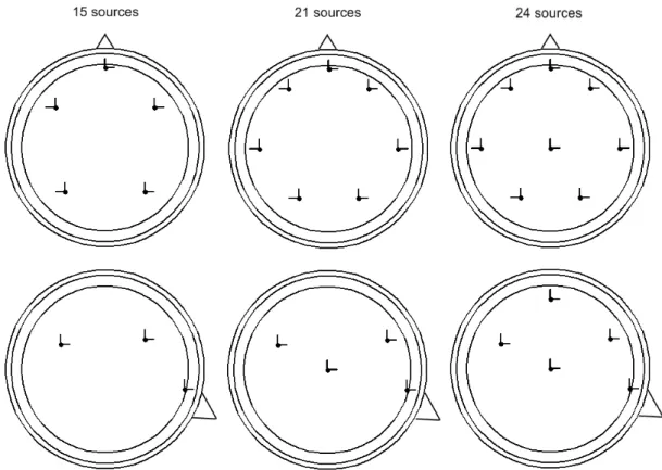
First, epochs containing other artifacts than the TMS artifact, and disconnected channels were excluded from analysis. The data were filtered with a second-order 2– 100-Hz Butterworth band-pass filter. The artifact topographies were defined by computing the principal components of an artifact-containing time period, the 5, 10, 15, 30, or 40 ms after the artifact, in the filtered and averaged data. One, two, and three eigenvectors corresponding to the highest eigenvalues were tested to define the artifact. The activity originating in the brain was simulated by a surrogate model, with 15, 21, or 24 source dipoles. The models had 5, 7, or 8 source locations, respectively, each with three orthogonal dipoles. The 15-source model was adapted from the one used by Berg and Scherg [20]. The 21-source model was formed by adding two temporal source locations to the 15-source model and moving the sources slightly outward. In the 24-source model, a dorsal 24-source location was added to the midline. The 24-source locations of the models are presented in Figure 4. The brain source topographies were defined by computing the potential at each electrode when each of the dipolar sources of the surrogate model was active. The field calculations were made assuming a spherical head model [52] (parameters from [53]). The columns of the resulting matrix formed the topographies of the sources. The chosen number of TMS components and the brain source topographies were combined to form the lead field matrix, and a Moore–Penrose pseudoinverse of the matrix was calculated using 0.00001 as the tolerance value. The

(20)

source wave forms were obtained as the product of the inverse matrix and the filtered data. The source wave forms were computed separately for all epochs and not the averaged data. The source wave forms corresponding to the artifact topographies were set to zero and the corrected data were computed as the product of the original lead field matrix and the artifact-free source matrix.

In the study of Litvak et al. [31], a new brain activity source model was calculated based on the global average of many subjects and this model was used instead of the surrogate model in the second round of the correction. However, as we only had data from one subject, this stage of the analysis was not implemented in this work.

The effect of the artifact-defining time period and the number of included TMS artifact topographies were evaluated by correcting the data from site 3 with 5, 10, 15, and 40 ms artifact defining period and one, two, and three artifact topographies. The 15-source surrogate model was used in all conditions. The artifact size was measured with each combination of parameters, by taking the square sum and maximum amplitude in the time period of 0–40 ms after the pulse. The deviation of the corrected signal from the original was calculated as described in ICA analysis (section 2.3.3), but for the time period of 40–300 ms after the TMS pulse.

The number of sources in the surrogate model was studied using 10 ms artifact defining period and three source topographies. Surrogate models containing 15, 21, and 24 sources were tested on the data from site 3.

To assess the effectiveness of the artifact removal method on data with lower artifact more comparable to the data used by Litvak et al. [31], the data from site 2 were corrected with 15 and 30 ms artifact-defining period, one, two, and three artifact topographies and the 15-source surrogate model. The analysis of the results was done as for the site 3 data.

(21)

Figure 4. Surrogate models with 15, 21, and 24 source dipoles. Top row presents the transverse view and bottom row the sagittal view. The triangles indicate the nose. The circles represent the surface of the brain, skull and skin in the spherical model.

(22)

3 Results

3.1 Artifact size depends on stimulation site and intensity

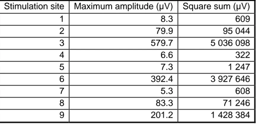
The size and shape of the artifact were measured in nine different sites on the left hemisphere. The square sums and maximum amplitudes are presented in Table 1. The stimulation sites close to the midline of the head (sites 1, 4, and 7 in Figure 1) gave the lowest maximum amplitude and square sums. The artifact size increased when more lateral areas were stimulated (sites 2, 3, 6, 8, and 9). The artifact was always strongest in the electrodes closest to the stimulation site.

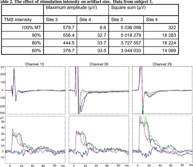
Stimulation intensity was tested on sites 3 and 4 of subject 1. As expected, the EEG response in site 3 was reduced, when lower stimulation intensities were used (Table 2). In site 4 the amplitude and square sum stayed quite constant, except in the 100% trial, which, surprisingly, had the lowest artifact. Stimulation intensity affected the duration of the artifact in various ways depending on the recording electrode and the stimulation site. When site 3 of subject 1 was stimulated (Figure 5, top row), the general shape of the artifact in channels 13 and 29 (opposite hemisphere and the top of the head) remained unchanged, and just the artifact amplitude was reduced. However, in channel 26, which is located relatively laterally on the same hemisphere as the stimulation site, the artifact was also shorter in duration when lower intensities (80 or 60%) were used. In channel 13, it can be seen that some of the early components of the artifact are reduced with the decreasing stimulation intensity. In site 4 of subject 1 (Figure 5, bottom row), the shape of the artifact wave form was more consistent between the electrodes. With the exception of the 100% MT stimulation exam, the duration of the artifact seemed to decrease with the stimulation intensity although the amplitude of the artifact stayed the same. Channel 29 was closest to the stimulation site.

Table 1. Effect of the stimulation site on artifact size. The stimulation sites are shown in Figure 1.

Stimulation site Maximum amplitude (µV) Square sum (µV)

1 8.3 609 2 79.9 95 044 3 579.7 5 036 098 4 6.6 322 5 7.3 1 247 6 392.4 3 927 646 7 5.3 608 8 83.3 71 246 9 201.2 1 428 384

(23)

Table 2. The effect of stimulation intensity on artifact size. Data from subject 1.

Maximum amplitude (µV)

Square sum (µV)

TMS intensity Site 3 Site 4 Site 3 Site 4

100% MT 579.7 6.6 5 036 098 322

90% 556.4 32.7 5 018 279 18 283

80% 444.5 33.7 3 727 557 18 224

60% 378.7 33.5 3 044 033 14 069

Figure 5. Artifact waveforms in subject 1 when site 3 (top row) and site 4 (bottom row) were stimulated. Blue line represents the experiment with 100%, black 90%, green 80%, and magenta 60% MT stimulation. Note the different y axis scale in the top and bottom rows.

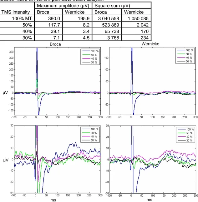
At lower intensities, the artifact was reduced even more both in amplitude and duration. The maximum amplitudes and square sums decreased more steeply with the intensity than when higher intensities were compared. In Broca’s area the decrease continued to the lowest intensity used, but the responses in Wernicke’s area settled on a low level already at 50% MT and did not decrease much further (Table 3). The decrease in artifact duration, visible also in the square sums, is best seen in Figure 6. When Broca’s area was stimulated, the duration of the artifact decreased steadily with the stimulation intensity, whereas when stimulating Wernicke’s area, the slowly decaying part of the artifact was only present in the 100% stimulation. The amplitude of the brain response is slightly reduced but still present in the lower-intensity experiments. In fact, when Broca’s area was stimulated with 30% MT, there was an additional peak in EEG around 30 ms, which was still partly covered by the artifact with higher-intensity stimulation.

(24)

Table 3. Artifact size when low intensity stimulation was used. The data from subject 2 has been filtered with a 100 Hz low pass filter before analysis.

TMS intensity

Maximum amplitude (µV) Square sum (µV)

Broca Wernicke Broca Wernicke

100% MT 390.0 195.9 3 040 558 1 050 085

50% 117.7 8.2 523 869 2 042

40% 39.1 3.4 65 738 170

30% 7.1 4.5 3 768 234

Figure 6. Effect of stimulation intensity on the global average EEG when Broca’s (left panels) and Wernicke’s (right panels) areas were stimulated. The upper figures show the effect of stimulation intensity on the overall size of the artifact, and the lower figures illustrate the effect on the artifact duration.

The effect of hemisphere on the EEG artifact was examined by analyzing data from a previous pilot study. In that subject, the maximum amplitude was always higher when the right hemisphere was stimulated. This was also true for the square sum in all but one case (Table 4).

(25)

Table 4. Effect of laterality on the artifact size.

left right left right

Broca 1 110.2 738.9 373 734 4 550 624

Speech arrest 305.7 739.9 2 033 509 6 996 807

Wernicke 1 321.8 538.9 2 329 620 3 459 528

Wernicke 2 331.3 490.7 2 683 991 2 588 863

Wernicke 3 370.4 574.3 2 576 108 2 993 824

3.2 Increasing amplifier gating time reduces artifact amplitude but

not duration

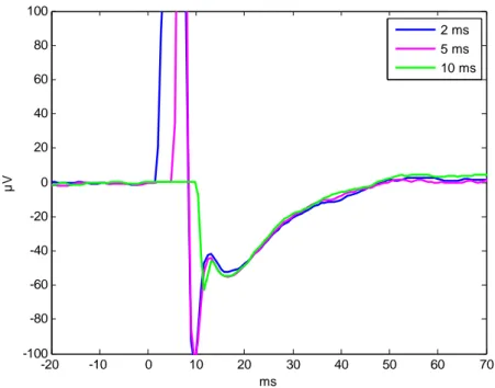
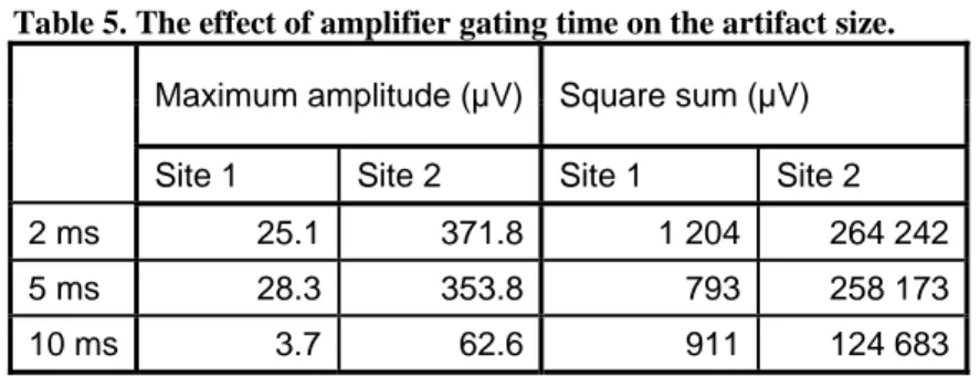
The data were corrupted by eye blinks and many trials had to be excluded to clear it but 41 to 63 trials were retained for each condition. Because the signal was held constant during the amplifier gating time, the square sum and amplitude of the data during the first 15 ms after the pulse would not be comparable between gating times. Instead, the interval of 15–50 ms after the stimulus was evaluated. The muscle artifact in site 2 was

generally higher (Table 5) and longer in duration (about 50 ms) than in site 1 (about 10 ms). In both sites, the highest part of the artifact was cut off when the amplifier gating time was 10 ms, and the maximum amplitude was lower than with shorter times. There is no great difference between 2- and 5-ms gating times. Changing the gating time does not affect the duration of the artifact or the general shape of the response immediately after the artifact (Figure 7).

-20 -10 0 10 20 30 40 50 60 70 -100 -80 -60 -40 -20 0 20 40 60 80 100 ms µV 2 ms 5 ms 10 ms

Figure 7. The effect of amplifier gating time on artifact shape and size. Global average of the response across channels is plotted. The data are from site 2 of subject 2.

(26)

Table 5. The effect of amplifier gating time on the artifact size.

Site 1 Site 2 Site 1 Site 2

2 ms 25.1 371.8 1 204 264 242

5 ms 28.3 353.8 793 258 173

10 ms 3.7 62.6 911 124 683

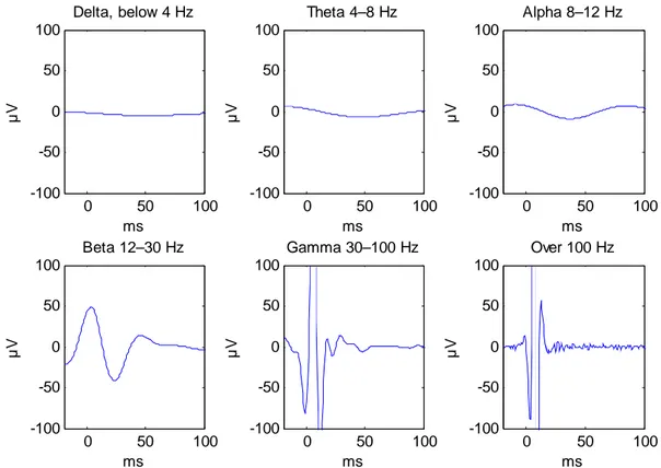
3.3 The artifact is strongest at higher frequencies

The frequency-band analysis was performed on the data of sites 3 and 4 of the stimulation site experiment. The data from site 3 are characterized by a high artifact, whereas the data from site 4 have a much lower response. In site 3, the highest components of the response are concentrated to the higher frequency bands: gamma and over 100 Hz (Table 6). The maximum amplitude is almost a hundred times higher in these bands than in the bands below 12 Hz. On the beta channel (12–30 Hz), the amplitude and the square sum is somewhat higher than in the lower bands, but still clearly smaller than in the two highest bands. The global average wave form of this band (Figure 8) looks like it contains some artifact activity (high regular spikes just after the pulse). In site 4, the power and maximum amplitude in all frequency bands is comparable. Only the delta and over 100 Hz bands are different from the other bands. On all channels the power and maximum amplitude is lower than in site 3.

Table 6. Distribution of the early response to different frequencies.

Site 3 Site 4 Frequency band Hz Maximum amplitude (µV) Square sum (µV) Maximum amplitude (µV) Square sum (µV) Delta 0–4 3.1 3 594 0.5 7 Theta 4–8 3.4 2 279 1.3 34 Alpha 8–12 7.2 4 568 1.6 53 Beta 12–30 49.3 222 119 1.3 41 Gamma 30–100 211.5 1 729 980 1.5 42 100– 339.0 1 462 812 2.8 54

(27)

0 50 100 -100 -50 0 50 100 ms µV Theta 4–8 Hz 0 50 100 -100 -50 0 50 100 ms µV Alpha 8–12 Hz 0 50 100 -100 -50 0 50 100 ms µV Beta 12–30 Hz 0 50 100 -100 -50 0 50 100 ms µV Gamma 30–100 Hz 0 50 100 -100 -50 0 50 100 ms µV Delta, below 4 Hz 0 50 100 -100 -50 0 50 100 ms µV Over 100 Hz

Figure 8. EEG response in different frequency bands. The data are from site 3 of subject 1. The artifact activity is most pronounced in the two highest frequency bands.

3.4 Artifact correction by ICA

The artifact correction was performed on the data from sites 3 and 4 of subject 1. First, the components containing large peaks 0–15 ms after the stimulus were removed and two low-pass filters in the preprocessing stage were evaluated. Artifact size in the 0–15 ms interval after the pulse was clearly reduced compared with the original and filtered signals in all examined cases (Table 7). The 100-Hz low-pass filter was generally more effective in reducing the artifact than the 200-Hz filter, although in two cases (ICA 3 and ICA 4 of site 3, 200-Hz filter) the artifact values are very low in comparison with other analyses. In these cases, the initial artifact was removed quite effectively, but there were some large peaks outside the time interval under investigation.

Especially in the data from stimulation site 3, the high artifact peaks were not limited to the first 15 ms but lasted until about 40 ms after the pulse, and the late components of the artifact were retained in the corrected data (Figure 9, top row). Therefore, the analysis was repeated for site 3, this time classifying all strong peaks occurring 0–40 ms after the pulse as artifacts and also evaluating the artifact in this interval. As a result, the late artifact size was reduced (Table 8) and the shape of the later response was retained well compared with the 0–15 ms interval correction (Figure 9, bottom row).

(28)

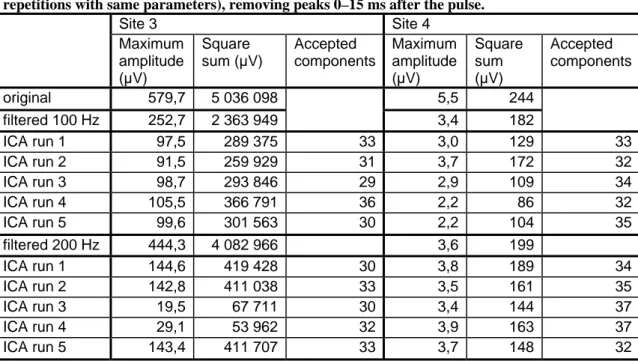
Table 7. Artifact size in the original data, filtered data and data corrected with ICA method (five repetitions with same parameters), removing peaks 0–15 ms after the pulse.

Site 3 Site 4 Maximum amplitude (µV) Square sum (µV) Accepted components Maximum amplitude (µV) Square sum (µV) Accepted components original 579,7 5 036 098 5,5 244 filtered 100 Hz 252,7 2 363 949 3,4 182 ICA run 1 97,5 289 375 33 3,0 129 33 ICA run 2 91,5 259 929 31 3,7 172 32 ICA run 3 98,7 293 846 29 2,9 109 34 ICA run 4 105,5 366 791 36 2,2 86 32 ICA run 5 99,6 301 563 30 2,2 104 35 filtered 200 Hz 444,3 4 082 966 3,6 199 ICA run 1 144,6 419 428 30 3,8 189 34 ICA run 2 142,8 411 038 33 3,5 161 35 ICA run 3 19,5 67 711 30 3,4 144 37 ICA run 4 29,1 53 962 32 3,9 163 37 ICA run 5 143,4 411 707 33 3,7 148 32

Table 8. The effect of ICA correction (five repetitions) when the components containing peaks 0–40 ms after the pulse were eliminated. The artifact is also evaluated in the period of 0–40 ms.

Site 3 Maximum amplitude (µV) Square sum (µV) Accepted components original 579.7 5 390 136 filtered 100 Hz 252.7 2 700 220 ICA run 1 16.7 9 837 30 ICA run 2 13.1 9 055 28 ICA run 3 16.3 13 928 31 ICA run 4 7.5 5 566 29 ICA run 5 14.2 9 337 30

The effect of ICA correction on the signal after the artifact peak was examined by plotting the original, filtered and corrected data together. The corrected signal followed the original least accurately in electrodes very close to the stimulation site (Figure 9, left panels), and most accurately on the opposite hemisphere far away from the coil (right panels). The middle panels depict signals from an electrode on the top of the head.

(29)

Figure 9. ICA corrected EEG wave forms in three channels (data from site 3, subject 1). Components having strong peaks in the 0–15 ms (top row), or 0–40 ms (bottom row) interval were removed. The blue line depicts the original signal, the green line the filtered and the red the corrected data.

When the FastICA parameters were adjusted, also the component topography was considered in addition to the wave form, and a longer sample was analyzed, better results than those presented in Table 8 were achieved in terms of the artifact removal and the distortion of the signal after the artifact using any combination of component number and function (Table 9). Examples of cleared data wave forms are given in Figure 10. The artifact is removed more efficiently than in the first analysis using 0–40 ms interval (Figure 9, bottom row) and less noise and deviation is added to the data outside the artifact period. Some examples of the independent components are given in Figure 11. Most of the components had topographies that were at least to some extent centered on the stimulation site, but the components classified as artifacts were the most polarized with little activity elsewhere. This strong polarization can be interpreted as a source located close to the head surface, such as the muscles.

(30)

Figure 10. Data corrected with the improved ICA method. Data from site 3 of subject 1, cleared with ICA using the symmetric approach, no PCA smoothing, 40 independent components, and

g(t)=t3 as the function. The blue line depicts the original signal, the green line the filtered and the

red the corrected data.

Figure 11. Examples of independent component classification. Top row: The components classified as brain activity have a distributed topography and no sharp peaks in the time interval of 0–40 ms. Bottom row: Artifact components have a more polarized topography and have peaks 0–40 ms after the TMS pulse.

(31)

Table 9. Comparison of ICA efficiency with different parameters. The artifact measured 0–40 ms after the TMS pulse. ICA-corrected data from subject 1 site 3 was averaged over 3 repeats of the analysis.

Maximum value (µV) t3 Tanh Gauss t2

Original 580 580 580 580

Filtered 253 253 253 253

30 Independent components 2 3 4 5

Square sum (µV) t3 Tanh Gauss t2

Original 5 390 136 5 390 136 5 390 136 5 390 136

Filtered 2 700 220 2 700 220 2 700 220 2 700 220

30 Independent components 366 359 940 1 064

40 Independent components 293 1 162 578 559

60 Independent components 672 1 221 1 129 4 348

Accepted components t3 Tanh Gauss t2

Deviation t3 Tanh Gauss t2

30 Independent components 209 637 151 916 134 867 187 490 40 Independent components 178 442 119 298 127 613 126 089

60 Independent components 71 042 78 634 97 242 98 381

According to the results averaged across the three analyses (Table 9), using 40 independent components seemed to give the lowest artifact, with the exception of the tanhfunction, where the lowest artifact was achieved using just 30 components. On the other hand, the lowest deviation from the original signal after the artifact was achieved using 60 components. In all conditions, 11–14 components were classified as artifact. The kurtosis function g(t)=t3 seemed to be the most effective in removing the artifact,

when 30 or 40 components were calculated, but the deviation is higher than when using other functions. There was still some variation between the analyses and therefore, these results are not conclusive. More repetitions and more accurate means of component classification are required to make real difference between the explored conditions.

3.5 Multiple-source analysis

Multiple-source correction of the TMS artifact was performed on the data of subject 1, stimulation sites 2 and 3. Combinations of different numbers of artifact topographies and artifact-defining time intervals were tested and the artifact size measured in each case. In all cases, the artifact size was reduced by about one decade (Table 10). The most effective combination that caused the least distortion of the signal after the artifact

(32)

was to use 3 artifact topographies and 10 or 15 ms time interval. To evaluate the effect of the correction to the signal outside the artifact-containing period, the corrected signal was plotted for each channel with the original and filtered data (Figure 12). In agreement with the numerical measurements, the artifact is reduced the most and the rest of the signal is least distorted when three artifact topographies are used. Examples of the artifact topographies when 10 ms artifact-defining periods are presented in Figure 13 and the topographies of the sources in the 15-source surrogate model are in Figure 14.

Figure 12. Data from three channels processed with the multiple-source correction. The blue line depicts the original signal, the green line the filtered and the red the corrected data.

Figure 13. The first five principal components of the TMS artifact calculated from the first 10 ms after the pulse. Numbers 1, 2 and 3 were used in correction.

(33)

Figure 14. The brain source topographies of the 15-source surrogate model.

Table 10. Comparison of the effect of artifact-defining time interval and the number of TMS artifact topographies on the multiple-source correction of data of subject 1, site 3.

Square sum (µV) 5 ms 10 ms 15 ms 40 ms Original 5 390 136 5 390 136 5 390 136 5 390 136 Filtered 2–100 Hz 2 700 220 2 700 220 2 700 220 2 700 220 1 artifact topography 229 818 186 255 165 387 162 384 2 artifact topographies 234 475 96 819 86 213 81 772 3 artifact topographies 239 378 68 024 73 190 57 330 Maximum amplitude (µV) 5 ms 10 ms 15 ms 40 ms Original 580 580 580 580 filtered 2–100 Hz 253 253 253 253 1 artifact topography 98 66 56 55 2 artifact topographies 160 70 56 60 3 artifact topographies 121 44 45 53 Deviation (µV) 5 ms 10 ms 15 ms 40 ms Original–filtered 31 023 31 023 31 023 31 023 1 artifact topography 103 026 124 997 121 384 118 900 2 artifact topographies 143 998 125 211 124 230 125 779 3 artifact topographies 143 740 107 206 119 073 124 307

Table 11. Effect of the surrogate model on the multiple-source correction of data from site 3 of subject 1.

15 sources 21 sources 24 sources

Maximum amplitude (µV) 44 196 203

Square sum (µV) 68 024 675 352 737 625

(34)

To assess the effect of the number of sources in the surrogate model, another experiment with 10 ms time interval and 3 topographies was performed. Adding model sources to the temporal areas close to the maximum artifact area could be argued to save some of the underlying neural activity but unfortunately this also preserved the artifact (Table 11).

To see how the method worked on data with a moderate artifact, that more closely resembles the data used in the study of Litvak et al. [31], an experiment was performed on the data of stimulation site 2, subject 1. Two time periods were used to determine the artifact, 15 ms was the duration of the first sharp peaks and 30 ms was the duration of the exponentially decaying part of the artifact evident on some channels. From the table it can be seen that the correction clearly reduces the artifact, there is no great difference between the time intervals of 15 and 30 ms, and that the artifact is reduced more when more artifact topographies are used (Table 12). However, the deviation of the corrected signal from the original after the artifact-containing period doubles when more than one topography are used. From the channel plots, it can be seen that although the artifact is further reduced, also the signal after it is distorted more from the original when two artifact topographies are used, compared with one (Figure 15).

Table 12. Multiple-source correction of a “moderate-artifact” data from subject 1 site 2.

Square sum (µV) 15 ms 30 ms Original 97 222 97 222 Filtered 2–100 Hz 48 061 48 061 1 artifact topography 4 458 4 403 2 artifact topographies 2 640 2 621 3 artifact topographies 1 256 1 401 Maximum amplitude (µV) 15 ms 30 ms Original 78 78 Filtered 2–100 Hz 28 28 1 artifact topography 18 17 2 artifact topographies 12 12 3 artifact topographies 7 7 Deviation (µV) 15ms 30 ms Original-filtered 23 897 23 897 1 artifact topography 24 250 24 195 2 artifact topographies 40 335 39 266 3 artifact topographies 41 431 40 597

(35)

Figure 15. Effect of the number of TMS artifact topographies on the signal wave forms of two channels. The data are from subject 1 stimulation site 2.

(36)

4 Discussion

4.1 Nature of the artifact

In experiments involving one subject, the artifact was found to be more pronounced when the stimulation was targeted to a lateral area, corresponding roughly to the distribution of muscles on the head (Table 1). The artifact was strongest in the channels close to the stimulation site, especially when the stimulation was close to the muscles. In theold data we used, it was noted that the artifact was much higher when the right, rather than the left side, was stimulated (Table 4). This could be due to the location of the reference electrode beneath the right ear in the experiment. [1] The positioning of the reference electrode should be considered carefully when both sides of the head are to be stimulated. The tests performed on the data of all three subjects were not strictly comparable with each other, since different parameters were used in the analyses, but the role of individual differences could and should be investigated in the current data. The artifact size decreased when the stimulation intensity was dropped to 90, 80, and 60% of MT, with one exception. The 100% MT stimulation of site 4 had, surprisingly, non-existent or at least much lower artifact than the lower intensities on the same site. This could be due to the fact that the 100% MT exam was made earlier than the lower intensity exams, and the impedance of the electrodes might have changed between the exams. The effect of stimulation intensity on artifact wave form depended much on the stimulation site. Whereas the duration was clearly affected in site 4, this effect was not so consistent in site 3. Instead, the early phases of the artifact were affected more. This, together with the observation that the artifact wave forms in sites 3 and 4 have different shapes, indicates that the artifacts generated in these sites have a different underlying mechanism. The artifact size was reduced even more when the stimulation intensity was dropped to 50, 40 and, 30% MT, especially in Broca’s area stimulation (Table 3). At 30%, also the duration of the artifact had been reduced enough so that the early response at 30 ms, masked by the late phase of the artifact with higher intensities, could be seen (Figure 6).

Although reducing the stimulation intensity reduces the artifact, it also leads to a diminished brain response. Komssi et al. [54] report that the threshold for neural excitation is around 40% MT in the motor cortex and some responses were recorded even after stimulation with only 20% MT stimulation. According to our data, even stimulation at 40% MT intensity still creates a high artifact in an artifact-prone stimulation site, the amplitude of which is above the TMS-evoked brain activity level (Table 2). In the planned language area study, the elicited brain activation should be strong enough to be transmitted to other areas. In previous studies using single-pulse

(37)

TMS to probe cortical connectivity, intensities of 80 [15, 30], 100% MT [15, 55, 56] or more [15, 57] have been used.

The artifact was also studied in terms of frequency content and was found to be most prominent in higher frequencies (Table 6). Most brain activity happens in frequencies lower than 100 Hz so frequencies higher than this can safely be filtered out. As is apparent from the ICA and multiple-source analyses in this study (Table 8, Table 10, Table 12), this sort of filtering alone is effective in reducing the size of the artifact, but is still not enough to remove it completely. Filtering out the lower artifact-containing frequencies (low pass 30 Hz) is expected to affect the brain signal also. However, it could be worth finding out whether the information contained in the lower frequency bins alone (below 30 Hz) would be valuable for the connectivity study.

The artifact shape in the channels with the strongest artifact can be divided into two phases: the first quick oscillation has a quite high frequency (about 80 Hz) and the late component decays exponentially, returning to zero only around 40–50 ms after the TMS pulse. The shape of the late artifact is not affected when the amplifier gating time is increased, indicating that the late artifact is not caused by problems in the amplifiers. At higher stimulation intensities (60–100% MT) the artifact duration changes more when a “low-artifact” site is stimulated but less consistently when a “high-artifact” site is stimulated (Figure 5). The shortening of the artifact duration with “high-artifact” stimulation site is better visible at lower intensities (Figure 6). The electrical artifact caused by the polarization of the skin–electrode interface would be expected not to depend on the stimulation site if the impedance of all included channels is comparable. This, together with the fact that the amplitude of the fast artifact is reduced evenly with stimulation intensity, suggests that the fast spikes of the artifact are of electrical origin.

4.2 Removing artifact from the recorded EEG data

Two methods of artifact removal were tested on the EEG data that contained artifacts: independent component analysis and multiple-source modeling. Although the methods produce a similar decomposition of the signals, the mixing matrix in ICA corresponds to the lead field matrix of the multiple-source model, and the independent components correspond to the source wave forms, the method of finding these matrices are completely different for these two methods. Whereas ICA is a purely mathematical approach, assuming only independence of the components, the multiple-source model uses information about the electrode locations, the assumed locations of the sources in the brain, and the spreading of electrical field patterns from the brain sources to the electrodes.

(38)

In this thesis, better results in terms of artifact removal and the distortion of the rest of the signal with the “high-artifact” data were delivered by ICA. Although accurate modeling of the head and voltage distributions would be expected to give better results, the assumptions in our multiple-source model clearly did not represent the reality well enough. The brain sources were modeled by a surrogate model with only five regional sources. I this way, some of the brain activity originating far away from the source locations might be lost. However, adding more sources to the surrogate model did not improve the correction, as observed also in [31], but rather worsened it. For the final correction round, Litvak et al. [31] used on the original data a surrogate model composed of sources calculated from the global average of data corrected with the 15-source model. Measuring more subjects and adding this step to our analysis could improve the results. The spherical head model presents another problem, especially in the lateral areas, where the head shape is not so well approximated by a sphere. The artifact is approximated by the first few eigenvectors calculated from an artifact-dominated time segment. The choice of this interval and the number of eigenvectors affect the results of artifact removal. Whereas in [31] one eigenvector was generally enough to represent the artifact, more were required to correct our “high artifact” data. We tested including up to three eigenvectors but perhaps even more could successfully be used, possibly adding eigenvectors as needed like in [31]. With the “moderate artifact” data, using only one eigenvector produced the best results.

The ICA method does not assume anything about the geometry or physics of the measurement setting. The assumption of independence, however, should be closely examined. Although the muscle artifact and brain activity are produced in different physiological structures with different mechanisms, they are temporally correlated close to the TMS stimulus. In the context of painful stimuli that might cause similar correlation between brain response and muscle artifact, Vigário et al. [26], [28] argue that this does not violate the independence assumption too much, if the data also contains enough noncorrelated muscle and brain activity.

The number of data points limits the number of components that can be estimated by ICA; trying to separate too many components can lead to overlearning [22]. This probably explains at least some of the improvement in results when the different running options were tested (1451 time points), compared with the results of the filtering tests (871 time points). Other differences between the filtering and running option tests were the approach (deflation and symmetric, respectively), the artifact selection method (component wave form and component wave form + topography) and the number of included eigenvectors in the whitening stage (40 and 60). With the latter parameters, the size of the artifact could be reduced to almost nothing. However, the