Modeling of 3D Flow and Scouring around Circular Piers
CHIN-LIEN YEN*,**, JIHN-SUNG LAI**, AND WEN-YI CHANG*,**
*Department of Civil Engineering National Taiwan University
Taipei, Taiwan, R.O.C. **Hydrotech Research Institute
National Taiwan University Taipei, Taiwan, R.O.C.
(Received January 24, 2000; Accepted May 4, 2000)
ABSTRACT
By combining a three-dimensional (3D) flow model with a scour model, a morphological model has been constructed to simulate the flow field and bed evolution around bridge piers. The large eddy simulation (LES) approach with Smagorinsky’s subgrid-scale (SGS) turbulent model is employed to compute 3D flow velocity and bed shear fields. For relatively coarse bed materials, the scour model solves the sediment continuity equation in conjunction with van Rijn’s bed-load sediment transport formula to simulate the bed evolution. Without recomputing the 3D flow field as the bed deforms, the shear field obtained from the 3D flow model under flatbed conditions is modified according to the bed deformation. The 3D flow model is verified with experimental data obtained under flatbed conditions. The gravitational effect of the sloping bed of the scour hole on sediment particle movement is incorporated as part of the effective bed shear stress in the scour model. The scouring effect resulting from downflow in the region in front of the pier is included in the model by referring to the vertical jet flow scour relation. The measured data of scour evolution at the pier nose obtained by R. Ettema and bed elevation contours around a pier obtained by G. H. Lin are used for calibration and verification of the model. The results show good agreement between simulation and experimental nesults.
Key Words: pier, scour, 3D flow, downflow, bed shear stress
I. Introduction
As water flow approaches a bridge pier, it is forced to separate and pass around the pier. The flow phenomena are complex due to the presence of a boundary layer as well as an adverse pressure gradient set up by the bridge pier. Consequently, the mechanism of the local scouring processes is complicated by 3D flow patterns, such as horseshoe vortex and downward current (downflow), and bed shear distribution around the pier. Many researchers have conducted a vast number of experiments in laboratory flumes to investigate the local scour depth around a bridge pier. Quite a few empirical formulas predicting the maximum scour depth have been developed under various experimental conditions. However, most of the experiments have been carried out in flumes under idealized conditions, such as steady flow, uniform sediment, simplified geometry, etc. (Ettema, 1980; Chiew and Melville, 1987; Lin, 1993). Therefore, their applications to field situ-ations may still be problematic and may produce questionable results. A more satisfactory approach for further applications in field situations is to simulate accurately the flow field and scouring processes using a 3D numerical model. Modeling 3D flow field and scour hole evolution around a bridge pier is more feasible nowadays because the computational cost and
computational time have significantly decreased.
Never-theless, three more coefficients in the function of the sediment transport capacity for local scouring need to be determined. Roulund et al. (1999) simulated the scouring processes over only a very short duration (5 minutes) by using a 3D flow model and solving the sediment continuity equation with Engelund’s bedload transport formula (Engelund, 1966). Tseng
et al. (2000) investigated numerically the 3D turbulent flow
field around square and circular piers. The simulated results they obtained indicated that the velocity and shear stress around the square pier were significantly higher than those around the circular pier. According to the aforementioned researches, the computational cost and time are still the major limitations for further applications when these models are used.
In the present study, a morphological model consisting of a 3D flow model and a scour model was developed to simulate the bed evolution around a circular pier. In order to reduce the computational time involved in repeatedly re-computing the 3D flow field as the bed scouring process progresses, an algorithm was developed to modify the bed shear field in order to account for bed deformation due to scouring. For the flow model, the simulated 3D flatbed flow field is compared here with experimental data obtained by Yeh (1996). In the scour model, the gravity effect of the sloping bed of the local scour hole is incorporated as part of the effective bed shear and verified by experimental results. Furthermore, in order to simulate the scouring process resulting from downflow in front of the pier, a relationship based on sub-merged jet flow scouring (Clarke, 1962) has been modified and employed. The experimental data for the scour depth at the pier nose obtained by Ettema (1980) and scour depth contours obtained by Lin (1993) are compared with simulated results obtained in this study to check the validity of our model.
II. Three-Dimensional Flow Model
1. Velocity Field
In order to describe the complex 3D flow patterns, including downflow in front of the pier and a horseshoe vortex around the circular pier, the weakly compressible flow theory (Song and Yuan, 1988) was employed. The large eddy simu-lation (LES) approach incorporated with Smagorinsky’s subgrid-scale (SGS) turbulence model was adopted to simulate the flow and bed shear fields (Song and Yuan, 1990). The LES approach has gained wider acceptance for solving hy-draulic problems because the SGS turbulence model is less dependent on the model coefficient than the κ-ε turbulence model (Thomas and Williams, 1995). The mathematical expressions for the weakly compressible flow equations, LES approach, SGS turbulence model, boundary conditions and numerical approach in explicit finite volume method based on MacCormack’s predictor-corrector scheme are given in the Appendix.
2. Bed Shear
Generally speaking, the bed shear stress (τij) can be
calculated using the following equation (Nezu and Rodi, 1986):
where µ is the dynamic viscosity; ui is the time-averaged
velocity component; and −ρui′u′j is the Reynolds’ stress. For a hydraulically smooth bed, the Reynolds’ stress term in the viscous sublayer is much smaller than the viscous shear stress term. Hence, the Reynolds’ stress term is negligible, and the bed shear stress can be calculated directly as follows:
τij=µ(
∂ui
∂xj + ∂uj
∂xi) (2)
In order to calculate the bed shear stress using Eq. (2), the size of the grid mesh adjacent to the bed must be kept smaller than the thickness of viscous sublayer.
To make possible the bed shear modification made to take into account bed deformation during scouring, Taylor series expansion is applied to the logarithmic velocity profile for bed deformation of ∆Z. This leads to (Yen et al., 1997)
U
u*=
U
u* +Dz, (3)
in which U is the modified depth-averaged velocity after bed deformation; u* is the modified shear velocity after bed deformation; U is the depth-averaged velocity before bed deformation; u* is the shear velocity before bed deformation;
Dz = 2.5[∆RZ – 12(∆RZ)2] ; and R is the water depth before bed
in which τ is the modified bed shear stress after bed deformation; and τ is the bed shear stress before bed deformation.
Strictly speaking, the velocity profile in the region close to the pier no longer satisfies the logarithmic distribution. Therefore, Eq. (4) can only be applied in the region some distance away from the pier. However, the ratio of the modified bed shear to the original bed shear in the vicinity of the pier is assumed to be the same as that in the region with the logarithmic velocity profile.
III. Scour Model
1. Bed Evolution
solving the sediment continuity equation with a sediment transport relation. Assuming that scouring takes place in the form of bedload transport, one can write the 2D sediment continuity equation as
and y-directions, respectively; λn is the sediment porosity; and
Zbis the bed elevation.
For coarse bed materials, sediment basically moves by rolling, sliding or jumping along the bed. The widely used bed-load sediment transport formula proposed by van Rijn (1986) is employed in the present study. van Rijn’s bed-load transport formula is expressed as
qs= 0.053 Ss′g d1.5T* 2.1
D*0.3, (6)
where qs is the sediment volume transport rate per unit width;
Ss′ = (Ss− 1); Ss is the specific gravity of the sediment; g is
the gravitational acceleration; d is the sediment diameter, T*
= (τb−τc)/τc, which is called the transport stage parameter; τb
, which is called the particle parameter; and µ
is the dynamic viscosity.
To solve Eq. (5), open and solid boundary conditions are imposed. The upstream inflow boundary condition is given by qsx = qsy = 0 for clear water scour. The downstream outflow
boundary condition is also given by qsx = qsy = 0 because at
some distance downstream, the flow becomes uniform again. For solid and lateral boundaries, no sediment flux conditions (qsn = 0, where qsn is the transport rate in the direction normal
to the boundaries) are imposed.
2. Effect of Local Bed Slope
In order to apply the sediment transport formula appro-priately in the scour hole with a sloping bed, the gravitational component along the bed surface is considered here as a part of the effective shear stress driving the motion of the sediment particles. On the sloping bed of the scour hole, the direction of sediment motion may not coincide with the direction of bed shear due to the flow motion; it is determined by the immersed weight of the sediment particle and the bed shear on the particle. In the direction of sediment motion, therefore, the effective shear stress empolyed in van Rijn’s bed-load transport formula is expressed as
τbe = τb× cos(β−δ) + w' × sinθ× cos(αd−δ)/A, (7)
where τbe is the effective shear stress; τb is the bed shear stress
due to the flow motion; β is the angle between the direction of bed shear and the x-axis; δ is the angle between the direction
of sediment motion and the x-axis, and can be evaluated using a method given elsewhere (Yen et al., 1997); w' is the immersed weight of the sediment particle; θ is the angle of the local bed slope; αd is the angle between the direction along the local
sloping bed and the x-axis; and A is the projected area of the sediment particle.
In Eq. (7), the first term on the right hand side represents the effective bed shear due to flow along the direction of sediment motion, and the second term represents the effective immersed sediment weight component, again along the direc-tion of sediment modirec-tion.
Considering a sediment particle on the sloping bed in the flow, the friction force Ff opposite to the direction of
incipient sediment motion is proportional to the normal force
N. Since the friction force per unit area of incipient motion is equal to the critical effective shear stress τc, one can write
τc = Ff /A = kfN/A, (8)
where kf is the friction coefficient, which is equal to tanφw,
and φw is the repose angle of sediment particles in still water.
In Eq. (8), the normal force N acting on a sediment particle includes the immersed sediment weight component
w'cosθand the lift force FL caused by the flow. Therefore, which reduces the normal force acting on a sediment particle and is obviously dependent on the local bed slope angle θ. When θ becomes large, the mean flow velocity becomes smaller due to the effects of increasing water depth and flow separation; consequently, the lift force decreases. Therefore, the coefficient m(θ) becomes smaller as θ increases. Another special case which needs to be considered is m(θ) = 0, and the remaining Eq. (9), tanφww′
Acosθ, simply represents the
critical shear stress for sediment particles on the sloping bed in still water. The coefficient m(θ) can be calibrated in the model.
3. Effect of Downflow
the evolution of the scour depth in the area in front of the pier. Clarke (1962) studied the scour depth evolution gen-erated by submerged vertical jet flow and proposed the fol-lowing relations:
where ysd is the scour depth generated by submerged vertical
jet flow; Dc is the diameter of the scour hole; Du is the diameter
of the jet flow; wo is the exit velocity of jet flow; t is time;
and ω is the sediment particle fall velocity.
In the present study, the downflow is considered analo-gous to the submerged vertical jet flow. The jet flow exit velocity wo is replaced with the maximum downflow velocity
(downflow strength) wm, and the scour depth ysd generated
by the jet flow is replaced with the downflow scour depth dj.
Since the characteristics of the downflow strength which develope near the bed surface are somewhat different from those of the jet flow, Eq. (10) is modified by introducing a coefficient C1. Thus, one has
In the present study, α is a coefficient that needs to be calibrated in the scour model. Rouse’s experimental results (Rouse, 1949) are used to establish a relationship between γ
and wm as follows:
γ= 0.03wωm + 0.078 . (13)
Furthermore, Ettema’s experiment results (Ettema, 1980) are employed to develop, by regression, a relationship between the downflow strength and the scour depth at the pier nose:
wm/wmo = 1 − 0.33(ds/b), (14)
where wm is the downflow strength for a scour hole having
a depth of ds at the pier nose; wmo is the downflow strength
under flatbed conditions; and ds/b is the ratio of the scour depth
to the pier diameter. (Note that ds/b is negative.)
In the present study, Eq. (11) is incorporated into the scour model. The increase in scour depth due to downflow,
∆dj, in one time step can be calculated using Eq. (11) first,
and then the bed deformation due to the effective shear stress,
∆Zb, in the same time step can be computed using Eq. (5) with
the bed-load transport formula. The final bed elevation at the pier nose, ds, is the sum of ∆dj and ∆Zb for all time steps.
4. Numerical Treatment
For numerical computation in the scour model, Eq. (5) is transformed into a conservative form as follows:
∂Zb
∂t +∇ ×Hs= 0 , (15)
where Hs= 1 1 –λn
[qsx,qsy] .
By integrating over a finite control area and invoking the divergence theorem, Eq. (15) becomes
∂Zb
∂t = – 1As ΓHs× n dΓ, (16)
where Zb represents the averaged elevation within the finite control area; As is the area of the finite grid mesh; n is unit
vector normal to the line of grid mesh; and Γ is the perimeter of the finite control area.
By using the forward difference in time, the bed elevation (Zb)m+ 1 in the advanced time step can be calculated as follows:
(Zb)m+ 1= (Zb)m–
∆ts
As Γ Hs× n dΓ, (17)
where the subscript m represents computational time, and ∆ts
is the time step adopted in the scour model.
IV. Verification of the Local Bed-Slope
Effect
To verify the gravity effect of the local bed slope in a scour hole, as described in the scour model (see Section III), several experiments were carried out in the present study. The experiments were conducted in a box 60 cm long by 20 cm wide. The box was first filled partially with sand with a mean diameter of 1.3 mm. The initial bed slope was set at 45° and sustained by a thin plate. Then water was slowly poured into the box, and the plate was quickly but carefully removed. After removal of the plate, sediment particles began to move down the slope mainly due to its gravitational component. The final stabilized bed slope was found to be at approximately the angle of repose of sediment in water.
initial and final bed profiles for all the runs are plotted in Fig. 1. The evolution of the bed elevation above the toe of the initial sloping bed (see point A in Fig. 1) is plotted in Fig. 2. As can be seen in Fig. 2, the bed elevation above point A increases rapidly during the early stage, and then begins to level off at about 1.5 sec.
Numerical simulation for the experiments described above was carried out under an initial bed slope of 45°. The bed profile evolution was simulated by solving Eq. (5) incor-porated with Eq. (6). In the simulation, the effective shear stress was calculated using Eq. (7), and the critical shear stress was calculated using Eq. (9). It was assumed that the mean velocity caused by the removal of the plate was negligible, and that eddies generated by the plate decayed very rapidly. Under these assumptions, the value of τb in Eq. (7) was taken
as zero. For the critical effective shear stress τc, the coefficient
m(θ) in Eq. (9) representing the effect of eddies on the reduction of the normal force was mainly dependent on the decay time of eddies rather than on the change of θ. The initial value of m(θ) was calibrated to 0.91, which corresponded to τc =
0.74 N/m2
obtained from the Shields diagram, and then m(θ) rapidly approached zero as eddies died out due to their rapid
decay. The simulated bed profile at t = 2 sec. and the evolution of the bed elevation above point A are plotted in Figs. 1 and 2, respectively. In Fig. 2, one can see that the simulated bed evolution and equilibrium time (at 1.5 sec) agree well with the measured data. These results clearly show that treating the gravitational component along the sloping bed of the local scour hole as a part of the effective shear stress driving the motion of the sediment particle is quite reasonable.
V. Flow Field Simulation
For validation of the 3D flow model, the experimental results obtained by Yeh (1996) were compared with simulation results. The conditions for the experiment were as follows: the pier diameter b = 0.031 m; the approaching surface velocity
uo = 0.126 m/s; the approaching water depth ho = 0.082 m;
the bed slope So = 0.0013; and the bed shear velocity u* =
6.83 × 10⁻³
m/s.
Numerical simulation was carried out under the condi-tions stated above. A structured grid mesh on the x-y plane was generated by an elliptic grid generator (Tseng, 1994). As shown in Fig. 3, a two-dimensional grid mesh with 60 elements in the x-direction and 36 elements in the y-direction was drawn, and there were 22 elements of nonuniform size in the z-direction. The smallest grid element was 0.028b × 0.021b × 0.003b. The simulation domain was −2 ≤ x/b ≤ 9.5, −2 ≤ y/b ≤ 2, and 0 ≤ z/b ≤ 2.65. The upstream boundary condition was given by the measured velocity profile along the z-direction. The downstream boundary condition was given by the Neumann condition (∂u/∂x = ∂v/∂x =∂w/∂x = 0). The boundary condition on the sides (i.e., y/b = ±2) was given by the fully slip condition (∂u/∂y = ∂w/∂y = 0 and v = 0). For the solid boundary condition, the cells adjoining the bed were given by the no-slip condition, and the cells adjoining the pier surface were prescribed by the partial slip condition in order to consider the variation of the local thickness of boundary layer relative to the local cell size (Song and Yuan, 1990). A value of 0.13 for the Smagorinsky constant was selected, which was within a reasonable range (0.094 ~ 0.2) for solving open channel flow problems (Thomas and Williams, 1995).
Some of the simulated results are plotted in Figs. 4 −
6. Since the flow field at section x/b = 9.5 is almost the same
Fig. 1. Simulated and measured bed profiles.
Fig. 2. Bed evolution at point A.
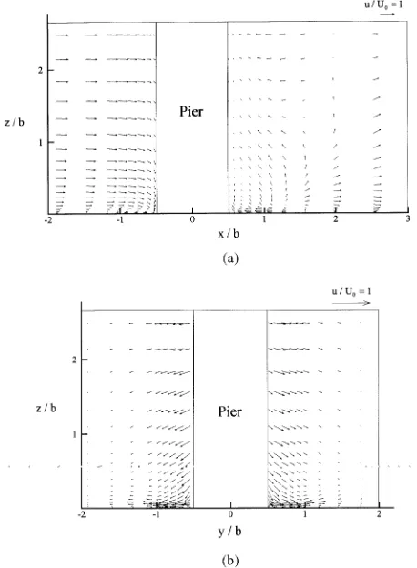
as that of the upstream inflow, the simulated results are only plotted within the range of −2 ≤ x/b ≤ 3 in the x-direction to clearly show the detailed flow field around the pier. Figure 4(a) shows the simulated velocity field on the vertical plane section (x-z plane) along the centerline. A downflow along a vertical line near the pier nose and a circulation area, as a component of a horseshoe vortex, close to the bed can be clearly seen. Figure 4(b) shows the simulated velocity field on the vertical plane (y-z plane) 90° from the centerline. One can clearly see that the velocity near the bed is enhanced. This may have significant implications for the initial stage of scouring.
Figure 5(a) presents the simulated velocity field on the horizontal plane at z/b = 0.032. It clearly shows that reverse flow exists in front of the pier. A comparison between the measured and simulated isovels at z/b = 0.032 above the bed, presented in Fig. 5(b), indicates good agreement between them. From these results, one can see that the 3D flow model can simulate flow features around the pier very well.
Upon obtaining the velocity field, the bed shear stresses were computed in the 3D flow model using Eq. (2). The simulated bed shear stresses along the centerline upstream of the pier are plotted in Fig. 6 and compared with the measured
data (Yeh, 1996). Another simulated result plotted as the dotted-line in Fig. 6 is from a previous work (Yen et al., 1997). It is based on the assumption that the velocity profile is of
Fig. 4. (a) Simulated velocity field on the vertical plane section (x-z plane) along the centerline. (b) Simulated velocity field on the vertical plane (y-z plane) 90° from the centerline.
Fig. 5. (a) Simulated velocity field on the horizontal plane at z/b = 0.032. (b) Comparison of simulated (upper half) and measured (lower half) isovels on the horizontal plane at z/b = 0.032 around the pier.
logarithmic distribution for computation of the bed shear, and it does not fit the measured data in the region of −1.5 <
x/b < −0.5. In this region, one can find that the bed shear stress varies from positive to negative at the point of flow separation, which is located approximately at x/b = −1.25. The location of this separation point, however, falls slightly up-stream from the range of −1.1 ≤ x/b ≤ −0.7 given by Graf and Yulistiyanto (1998). Nevertheless, the bed condition for the present simulation is hydraulically smooth (Yeh, 1996); hence, the turbulence intensity in the flow may not be strong enough to transfer sufficient momentum into the vicinity of the bed surface to push the separation point further downstream.
VI. Scour Simulation
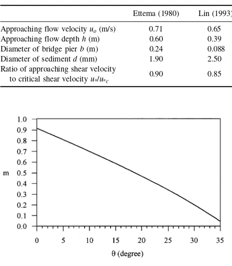
For calibration and verification of the scour model, the experimental conditions used and results obtained by Ettema (1980) and by Lin (1993) were employed for simulation and comparison. The flow and sediment conditions used in their experiments are listed in Table 1.
Ettema’s experiments were used to calibrate the model coefficients. After a 15-hour (tuo/b = 160,000) scour
simu-lation run, the coefficient α in Eq. (11) was calibrated and found to be 0.5, and the coefficient m(θ) in Eq. (9) was calibrated as shown in Fig. 7. In Fig. 8, the simulated scour depth at the pier nose as a function of time is compared with the measured data, and one can see rather good agreement
between them.
For verification of the scour model, the calibrated coefficients were used to simulate the scour depth evolution in Lin’s experiments. The simulated scour depth at the pier nose is plotted in Fig. 9, and the measured scour depth at 2 hours (tuo/b = 53,000) is also plotted in the figure to show
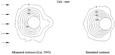
the good match. The ratio of the maximum scour depth to the water depth is about 1/6 in this case, and this parameter is mainly affected by the ratio of the approaching velocity to the critical velocity, the ratio of the particle diameter to the pier diameter, the ratio of the approaching water depth to the pier diameter, etc. Furthermore, the simulated and measured final bed elevation contours are shown in Fig. 10 for comparison. The scour hole extends around the circular pier with a deeper area at the upstream side and a shallower one downstream. With the exception of a small region on the downstream side, the simulated results of the scour pattern and maximum scour depth are satisfactory, and the overall simulation is fairly good. In the wake region close to the pier where turbulence is relatively strong, the effective critical shear stress for sediment motion may be significantly reduced. This fact has not been accounted for in the simulation model; therefore, the
simu-Table 1. Conditions of Experiments Adopted for Scour Simulations
Ettema (1980) Lin (1993) Approaching flow velocity uo (m/s) 0.71 0.65
Approaching flow depth h (m) 0.60 0.39
Diameter of bridge pier b (m) 0.24 0.088
Diameter of sediment d (mm) 1.90 2.50
Ratio of approaching shear velocity
0.90 0.85
to critical shear velocity u*/u*c
Fig. 7. Coefficient m(θ) calibrated by means of Ettema’s experiments.
Fig. 8. Comparison of simulated and experimental results of the scour depth evolution at the pier nose − a calibration run.
lation yields slightly less scouring in the small region behind the pier.
VII. Summary and Conclusions
The morphological model consisting of a 3D flow model with a scour model has been constructed to simulate the bed scour evolution around a bridge pier. For 3D flow modeling, the LES approach with Smagorinsky’s SGS turbulence model has been employed to compute the velocity and bed shear stress fields. In the scour model, the sediment continuity equation incorporated with van Rijn’s bed-load sediment transport for-mula for relatively coarse materials has been solved to obtain the bed evolution.
The 3D flow model has been validated using experi-mental data measured using a Fiber-Optic Laser Doppler Velocimeter under flatbed conditions (Yeh, 1996), and a Smagorinsky constant of 0.13 was selected, which falls rea-sonably well within the range (0.094 ∼ 0.2) in open channel flow problems (Thomas and Williams, 1995). From the simulation results, it has been found that the 3D flow model can simulate the velocity field around the pier very well.
The effect of the local bed slope of the scour hole on the direction of sediment particle motion has been incorporated into the model as part of the effective shear stress. Experiments as well as simulation were conducted to verify this effect. The effect of downflow on the scour depth has also been included in the model by referring to the submerged vertical jet flow scour relation in order to improve the simulation in the area in front of the pier. The experimental data of the scour depth evolution at the pier nose obtained by Ettema (1980) and the scour depth contours obtained by Lin (1993) have been com-pared with the simulated results and show good agreement. On the basis of the results presented in the present study, the morphological model proposed herein is regarded as feasible for further applications in field situations.
Acknowledgment
The provision of research facilities for the study reported herein by
the Hydrotech Research Institute, National Taiwan University, R.O.C., is gratefully acknowledged. Financial support by the National Science Council, R.O.C., under grant NSC 86-2621-E-002-021 has been highly appreciated.
References
Chiew, Y. M. and B. W. Melville (1987) Local scour around bridge piers.
J. of Hydraulic Research, IAHR, 25, 15-26.
Clarke, F. R. W. (1962) The Action of Submerged Jets on Movable Material. Ph.D. Dissertation. Imperial College, London, U.K.
Dou, X. (1997) Numerical Simulation of Three-Dimensional Flow Field and Local Scour at Bridge Crossings. Ph.D. Dissertation. University of Mississippi, Oxford, MS, U.S.A.
Engelund, F. (1966) Hydraulic resistance of alluvial streams. J. of Hydraulic Division, ASCE, 92(HY2), 315-326.
Ettema, R. (1980) Scour at Bridge Piers. Rept. No. 216, University of Auckland, Auckland, New Zealand.
Graf, W. H. and B. Yulistiyanto (1998) Experiments of flow around a cylinder: the velocity and vorticity fields. J. of Hydraulic Research, IAHR, 36, 637-653.
Lin, G. H. (1993) Study on the Local Scour around Cylindrical Bridge Piers
(in Chinese). M.S. Thesis. Feng-Chia University, Taichung, Taiwan, R.O.C.
MacCormack, R. W. (1969) The effect of viscosity in hypervelocity impact cratering. AIAA J., 7, 69-354.
Nezu, I. and W. Rodi (1986) Open-channel flow measurements with a laser doppler anemometer. J. of Hydraulic Engineering, ASCE, 112, 335-355.
Olsen, N. R. B. and H. M. Kjellesvig (1998) Three-dimensional numerical flow modeling for estimation of maximum local scour depth. J. of Hydraulic Research, IAHR, 36, 579-590.
Olsen, N. R. B. and M. C. Melaaen (1993) Three-dimensional calculation of scour around cylinders. J. of Hydraulic Engineering, ASCE, 119, 1048-1054.
Richardson, J. E. and V. G. Panchang (1998) Three-dimensional simulation of scour-inducing flow at bridge piers. J. of Hydraulic Engineering, ASCE, 124, 530-540.
Roulund, A., B. M. Sumer, J. Fredsoe, and J. Michelsen (1999) 3D math-ematical modeling of scour around a circular pile in current. Proc., 7th Int’l Symposium on River Sedimentation and 2nd Int’l Symposium on Environmental Hydraulics ´98, Hong Kong, P.R.C.
Rouse, H. (1949) Engineering Hydraulics, pp. 786-789. Wiley, New York, NY, U.S.A.
Smagorinsky, J. (1963) General circulation experiments with primitive equation. Monthly Weather Review, 91, 99-154.
Song, C. and M. Yuan (1988) A weakly compressible flow model and rapid convergence method. J. of Fluids Engineering, ASME, 110, 441-445.
Song, C. and M. Yuan (1990) Simulation of vortex-shedding flow about a circular cylinder at high Reynolds number. J. of Fluids Engineering, ASME, 112, 115-163.
Thomas, T. G. and J. J. R. Williams (1995) Large eddy simulation of a symmetric trapezoidal channel at a Reynolds number of 430,000. J. of Hydraulic Research, IAHR, 33, 825-842.
Tseng, M. H. (1994) Numerical Simulation of Flow and Scour around Bridge Pier (in Chinese). Ph.D. Dissertation. National Taiwan University, Taipei, Taiwan, R.O.C.
Tseng, M. H., C. L. Yen, and C. S. Song (2000) Computation of three-dimensional flow around square and circular piers. International Journal for Numerical Methods in Fluids. (accepted)
van Rijn, L. C. (1986) Sediment transport, part 1: bed load transport. J. of Hydraulic Engineering, ASCE, 112, 433-455.
Yeh, J. C. (1996) The Flow Fields around Square and Circular Cylinders
Mounted Vertically on a Fixed Flat Bottom (in Chinese). M.S. Thesis. National Chung-Hsing University, Taichung, Taiwan, R.O.C. Yen, C. L., M. H. Tseng, and J. S. Lai (1997) Simulation of Bridge Scour
under Unsteady Flow (in Chinese). Rept. No. NSC 85-2211-E-002-051, National Science Council, R.O.C., Taipei, Taiwan, R.O.C.
APPENDIX
Basic Theory for 3D Flow Simulation
1. Governing Equations
According to weakly compressible flow theory (Song and Yuan, 1988, 1990), the Mach number in water flow is so small that the fluid density and sound speed may be regarded as constants without causing significant error. It is noted that weakly compressible flow is equivalent to hydraulic transient flow. Therefore, the equation of state for a fluid may be represented by the following linear relation:
p−po = ao2(ρ−ρo), (A1)
where p is the pressure; a is the speed of sound; ρ is the density of the fluid; and the subscript “o” represents the reference value.
Substituting Eq. (A1) into the equations of continuity and motion for compressible fluids, the equations become
∂p coefficient; and M is the Mach number.
When M << 1, the pressure term in Eq. (A2) is negligible and α ≈
Equations (A4) and (A5) are defined as weakly compressible flow equations, which were also used for hydraulic transient flow as the primary governing equations in the present study.
Generally speaking, Eq. (A5) also can be transformed into vorticity equation form and then can be solved to obtain the flow field. However, solving the vorticity equation to simulate the flow field around piers may be more difficult because the initial and boundary conditions are not easy to prescribe.
2. Large Eddy Simulation
For a high Reynolds number, the turbulent flow contains a wide range of eddy sizes. Herein, the concept of large eddy simulation (LES) is adopted so as to directly calculate the large-scale turbulence that can be resolved within the computational mesh size and to model only the unresolvable small-scale turbulence.
In the mesh grid, each flow variable f (velocity component ui or
pressure p) can be represented by an averaged quantity f plus a quantity
f ' related to subgrid scale turbulence, that is, f = f + f ' (f = 1
∆V ∆Vf(V,t)×dV,
where ∆V is the finite volume of the computational mesh grid and V is its volume). Based on the above relationship of the averaged quantity in the finite volume, the weakly compressible flow equations become (Song and Yuan, 1988) is the subgrid scale turbulence stress. The subgrid turbulence stress is modeled by the following relation (Smagorinsky, 1963):
τij= – 2ρυtSij, (A8)
where υt = (C∆s)2(2Sij Sij)
1/2
is the subgrid eddy viscosity coefficient;
Sij= 12(∂ui/∂xj+∂uj/∂xi) is the resolvable rate of deformation tensor; ∆s is the subgrid length scale dependent on the mesh size; and C is the Smagorinsky constant, which is the only adjustable parameter in the subgrid scale turbulence (SGS) model.
3. Boundary Conditions
To solve Eqs. (A6) and (A7), adequate boundary conditions should be imposed. Typical boundary conditions are described as follows:
(1)Upstream boundary condition:
where uo is the approaching velocity; pd is the averaged pressure downstream; and po is the reference pressure. In the present study, the downstream boundary condition is given by ∂∂ux=∂∂vx=∂∂wx = 0 ;
pd=po.
(3)Solid boundary condition: The fully slip condition, partial slip condition (wall function) or non-slip condition can be adopted ac-cording to the characteristics of the solid boundary (Tseng, 1994; Yen et al., 1997).
(4)Free surface boundary condition: The kinematic boundary con-dition or dynamic boundary concon-dition is imposed.
(i) For the kinematic boundary condition, the deformation rate of the water surface must equal the flow velocity normal to the water surface, i.e.,
∂Zf
∂t +u× ∇Zf=u×n on z = Zf (x,y,t), (A11)
where Zf is the elevation of the water surface; u is velocity vector; and n is the unit vector normal to the water surface. (ii) For the dynamic boundary condition, there is no momentum flux
through the water surface, i.e., σ
σijnij = 0 on z = Zf (x, y, t), (A12) where σσij is the stress tensor defined as σσij = −pδij + τij. 4. Numerical Approach
most compatible with the volume-averaged LES approach and has sufficient flexibility to fit irregular boundaries. In the framework of the finite volume method, MacCormack’s explicit predictor-corrector scheme (MacCormack, 1969), which is of second order accuracy in both time and space, is employed to solve the governing equations.
Equations (A6) and (A7) can be rewritten in a conservative form: ∂U
∂t +∂∂Ex +∂∂Fy +∂∂Gz = 0 , or ∂∂Ut +∇ ⋅H= 0 , (A13)
where
U = [p,u, v, w]T, H = [E, F, G],
E= [ρoao2u, u2+ p ρo–υ
∂u ∂x +
τxx ρo ,uv–υ
∂v ∂x +
τyx ρo ,
uw–υ∂∂wx +τzx ρo]
T ,
F= [ρoao2v,uv–υ∂ u ∂y +
τxy ρo ,v
2+ p
ρo–υ ∂v
∂y + τyy ρo ,
vw–υ∂∂wy +τzy ρo]
T,
G= [ρoao2w,uw–υ ∂u
∂z + τxz ρo , vw–υ
∂v ∂z +
τyz ρo ,
w2+ p
ρo–υ ∂w
∂z + τzz ρo]
T.
After integrating over a finite control volume ∆V and using the divergence theorem, Eq. (A13) can be replaced by
∂U
∂t =I, (A14)
where I = −∆1V H×n ds
s ; U represents a mean quantity within the finite control volume (the grid mesh size); and s is its finite control surface.
With MacCormack’s predictor-corrector scheme, Eq. (A14) can be approximated in two calculation steps as follows:
(1) the predictor step:
Um+ 1=Um+Im∆t; (A15)
(2) the corrector step:
Um+ 1=Um+ 12(Im+Im+ 1)∆t, (A16)
where Im+ 1= – 1∆V Hm+ 1×n ds
s ; the subscript m represents the computation time; and the hat ^ represents the predicted values. For numerical stability, the time step ∆t in Eqs. (A15) and (A16) must be determined by using the Courant-Friedrich-Lewy condition (Song and Yuan, 1988):
∆t≤Cr⋅Min[ ∆V uiΩi +aoΩ
] , (A17)
where Cr is the Courant stability factor with a value of 0.8 adopted in the present study; ui is the velocity vector; |Ω| is the surface area of the finite volume; and Ωiis the projected area of |Ω| in the i direction.
*,** ** *,**
large eddy simulation Smagorinsky
van Rijn