Boris Smus
Web Audio API
by Boris Smus
Copyright © 2013 Boris Smus. All rights reserved.
Printed in the United States of America.
Published by O’Reilly Media, Inc., 1005 Gravenstein Highway North, Sebastopol, CA 95472.
O’Reilly books may be purchased for educational, business, or sales promotional use. Online editions are also available for most titles (http://my.safaribooksonline.com). For more information, contact our corporate/ institutional sales department: 800-998-9938 or [email protected].
Editors: Simon St. Laurent and Meghan Blanchette Production Editor: Kara Ebrahim
Proofreader: Jilly Gagnon
Cover Designer: Randy Comer Interior Designer: David Futato Illustrator: Rebecca Demarest
March 2013: First Edition
Revision History for the First Edition:
2013-03-07: First release
See http://oreilly.com/catalog/errata.csp?isbn=9781449332686 for release details.
Nutshell Handbook, the Nutshell Handbook logo, and the O’Reilly logo are registered trademarks of O’Reilly Media, Inc. Web Audio API, the image of a brown long-eared bat, and related trade dress are trademarks of O’Reilly Media, Inc.
Many of the designations used by manufacturers and sellers to distinguish their products are claimed as trademarks. Where those designations appear in this book, and O’Reilly Media, Inc., was aware of a trade‐ mark claim, the designations have been printed in caps or initial caps.
While every precaution has been taken in the preparation of this book, the publisher and author assume no responsibility for errors or omissions, or for damages resulting from the use of the information contained herein.
ISBN: 978-1-449-33268-6
Table of Contents
Preface. . . vii
1. Fundamentals. . . 1
A Brief History of Audio on the Web 1
Games and Interactivity 2
The Audio Context 3
Initializing an Audio Context 4
Types of Web Audio Nodes 5
Connecting the Audio Graph 5
Power of Modular Routing 6
Loading and Playing Sounds 10
Putting It All Together 11
2. Perfect Timing and Latency. . . 13
Timing Model 13
Precise Playback and Resume 13
Scheduling Precise Rhythms 15
Changing Audio Parameters 15
Gradually Varying Audio Parameters 16
Custom Timing Curves 18
3. Volume and Loudness. . . 21
Equal Power Crossfading 23
Using Meters to Detect and Prevent Clipping 25
Dynamics Compression 28
4. Pitch and the Frequency Domain. . . 29
Pitch and playbackRate 31
Multiple Sounds with Variations 32
Oscillator-Based Direct Sound Synthesis 34
5. Analysis and Visualization. . . 37
Frequency Analysis 37
Animating with requestAnimationFrame 39
Visualizing Sound 40
6. Advanced Topics. . . 43
Adding Effects via Filters 44
Procedurally Generated Sound 45
Room Effects 47
Spatialized Sound 49
Audio Processing with JavaScript 51
7. Integrating with Other Technologies. . . 53
Setting Up Background Music with the <audio> Tag 53
Live Audio Input 54
Page Visibility and Audio Playback 55
8. Conclusion. . . 57
A. Deprecation Notes. . . 59
Preface
Thank you for picking up the first book on the topic of the Web Audio API. When I first learned of the Web Audio API, I was a complete digital-audio novice embarking on a journey to learn and understand the API, as well as the underlying fundamental audio concepts. This book is what I wish existed when I started experimenting with the API in 2011. It is intended to be a springboard for web developers like I was, with little to no digital-audio expertise. It contains the things I learned from about a year of study‐ ing digital audio processing, having conversations with audio experts, and experiment‐ ing with the API.
The theoretical bits will be filled in through asides, which will explain the concepts. If you are a digital-audio guru, feel free to skip these. The practical bits will be illustrated with code snippets to give you a better sense of how the API works in real life. Many of the examples also include links to working samples that can be found on this Web Audio API site.
Structure of This Book
This book aims to give a high-level overview of a number of important features of the Web Audio API, but is not an exhaustive survey of every available feature. It is not intended as a comprehensive guide, but as an easy starting point. Most sections of the book start off by describing an application, outlining the problem and solution, and then showing relevant sample JavaScript Web Audio API code. Interspersed theory sections explain some of the underlying audio concepts in more general terms. The book is structured in the following way:
1. Chapter 1, Fundamentals covers the basics of audio graphs, typical graph configu‐ rations, audio nodes inside those graphs, loading sound files, and playing sounds back.
2. Chapter 2, Perfect Timing and Latency delves into precise scheduling of sound in the future, multiple simultaneous sounds, changing parameters directly or over time, and crossfading.
3. Chapter 3, Volume and Loudness covers gain, volume, and loudness, as well as preventing clipping via metering and dynamics compression.
4. Chapter 4, Pitch and the Frequency Domain is all about sound frequency, an im‐ portant property of periodic sound. We’ll also talk about oscillators and examining sound in the frequency domain.
5. Chapter 5, Analysis and Visualization builds on the earlier chapters to dive into more advanced topics, including biquad filters, simulating acoustic environments, and spatialized sounds.
6. In Chapter 6, Advanced Topics, we will take a break from synthesizing and manip‐ ulating sound, and analyze and visualize sound instead.
7. Chapter 7, Integrating with Other Technologies talks about interfacing Web Audio API with other web APIs like WebRTC and the <audio> tag.
The source code of the book itself is released under the Creative Commons license and is available on GitHub.
Conventions Used in This Book
The following typographical conventions are used in this book: Italic
Indicates new terms, URLs, email addresses, filenames, and file extensions. Constant width
Used for program listings, as well as within paragraphs to refer to program elements such as variable or function names, databases, data types, environment variables, statements, and keywords.
Constant width bold
Shows commands or other text that should be typed literally by the user. Constant width italic
Shows text that should be replaced with user-supplied values or by values deter‐ mined by context.
This icon indicates a warning or caution.
Using Code Examples
This book is here to help you get your job done. In general, if this book includes code examples, you may use the code in your programs and documentation. You do not need to contact us for permission unless you’re reproducing a significant portion of the code. For example, writing a program that uses several chunks of code from this book does not require permission. Selling or distributing a CD-ROM of examples from O’Reilly books does require permission. Answering a question by citing this book and quoting example code does not require permission. Incorporating a significant amount of ex‐ ample code from this book into your product’s documentation does require permission. We appreciate, but do not require, attribution. An attribution usually includes the title, author, publisher, and ISBN. For example: “Web Audio API by Boris Smus (O’Reilly). Copyright 2013 Boris Smus, 978-1-449-33268-6.”
If you feel your use of code examples falls outside fair use or the permission given above, feel free to contact us at [email protected].
Safari® Books Online
Safari Books Online (www.safaribooksonline.com) is an on-demand digital library that delivers expert content in both book and video form from the world’s leading authors in technology and business. Technology professionals, software developers, web designers, and business and crea‐ tive professionals use Safari Books Online as their primary resource for research, prob‐ lem solving, learning, and certification training.
Safari Books Online offers a range of product mixes and pricing programs for organi‐ zations, government agencies, and individuals. Subscribers have access to thousands of books, training videos, and prepublication manuscripts in one fully searchable database from publishers like O’Reilly Media, Prentice Hall Professional, Addison-Wesley Pro‐ fessional, Microsoft Press, Sams, Que, Peachpit Press, Focal Press, Cisco Press, John Wiley & Sons, Syngress, Morgan Kaufmann, IBM Redbooks, Packt, Adobe Press, FT Press, Apress, Manning, New Riders, McGraw-Hill, Jones & Bartlett, Course Technol‐ ogy, and dozens more. For more information about Safari Books Online, please visit us online.
How to Contact Us
Please address comments and questions concerning this book to the publisher: O’Reilly Media, Inc.
1005 Gravenstein Highway North Sebastopol, CA 95472
800-998-9938 (in the United States or Canada) 707-829-0515 (international or local) 707-829-0104 (fax)
We have a web page for this book, where we list errata, examples, and any additional information. You can access this page at http://oreil.ly/web-audio-api.
To comment or ask technical questions about this book, send email to bookques [email protected].
For more information about our books, courses, conferences, and news, see our website at http://www.oreilly.com.
Find us on Facebook: http://facebook.com/oreilly
Follow us on Twitter: http://twitter.com/oreillymedia
Watch us on YouTube: http://www.youtube.com/oreillymedia
Thanks!
I am not an expert in digital signals processing, mastering, or mixing by any stretch. I am a software engineer and amateur musician with enough interest in digital audio to spend some time exploring the Web Audio API and wrapping my head around some of its important concepts. To write this book, I had to continually bug others with far more digital-audio experience than me. I’d like to thank them for answering my ques‐ tions, providing technical reviews for this book, and encouraging me along the way. Specifically, this book could not have been written without the generous mentorship of Chris Rogers, the primary author of the Web Audio specification and also its main WebKit/Chrome implementer. I owe many thanks to Chris Wilson, who gave an in‐ credibly thorough technical review of this book’s content, and to Mark Goldstein, who spent a few late nights doing editorial passes. My thanks to Kevin Ennis for donating webaudioapi.com for hosting samples related to the book. Last but not least, I would have never written this book without the support and interest of a vibrant Web Audio API community on the Web.
CHAPTER 1
Fundamentals
This chapter will describe how to get started with the Web Audio API, which browsers are supported, how to detect if the API is available, what an audio graph is, what audio nodes are, how to connect nodes together, some basic node types, and finally, how to load sound files and playback sounds.
A Brief History of Audio on the Web
The first way of playing back sounds on the web was via the <bgsound> tag, which let website authors automatically play background music when a visitor opened their pages. This feature was only available in Internet Explorer, and was never standardized or picked up by other browsers. Netscape implemented a similar feature with the <embed> tag, providing basically equivalent functionality.
Flash was the first cross-browser way of playing back audio on the Web, but it had the significant drawback of requiring a plug-in to run. More recently, browser vendors have rallied around the HTML5 <audio> element, which provides native support for audio playback in all modern browsers.
Although audio on the Web no longer requires a plug-in, the <audio> tag has significant limitations for implementing sophisticated games and interactive applications. The fol‐ lowing are just some of the limitations of the <audio> element:
• No precise timing controls
• Very low limit for the number of sounds played at once • No way to reliably pre-buffer a sound
• No ability to apply real-time effects • No way to analyze sounds
There have been several attempts to create a powerful audio API on the Web to address some of the limitations I previously described. One notable example is the Audio Data API that was designed and prototyped in Mozilla Firefox. Mozilla’s approach started with an <audio> element and extended its JavaScript API with additional features. This API has a limited audio graph (more on this later in “The Audio Context” (page 3)), and hasn’t been adopted beyond its first implementation. It is currently deprecated in Firefox in favor of the Web Audio API.
In contrast with the Audio Data API, the Web Audio API is a brand new model, com‐ pletely separate from the <audio> tag, although there are integration points with other web APIs (see Chapter 7). It is a high-level JavaScript API for processing and synthe‐ sizing audio in web applications. The goal of this API is to include capabilities found in modern game engines and some of the mixing, processing, and filtering tasks that are found in modern desktop audio production applications. The result is a versatile API that can be used in a variety of audio-related tasks, from games, to interactive applica‐ tions, to very advanced music synthesis applications and visualizations.
Games and Interactivity
Audio is a huge part of what makes interactive experiences so compelling. If you don’t believe me, try watching a movie with the volume muted.
Games are no exception! My fondest video game memories are of the music and sound effects. Now, nearly two decades after the release of some of my favorites, I still can’t get Koji Kondo’s Zelda and Matt Uelmen’s Diablo soundtracks out of my head. Even the sound effects from these masterfully-designed games are instantly recognizable, from the unit click responses in Blizzard’s Warcraft and Starcraft series to samples from Nin‐ tendo’s classics.
Sound effects matter a great deal outside of games, too. They have been around in user interfaces (UIs) since the days of the command line, where certain kinds of errors would result in an audible beep. The same idea continues through modern UIs, where well-placed sounds are critical for notifications, chimes, and of course audio and video com‐ munication applications like Skype. Assistant software such as Google Now and Siri provide rich, audio-based feedback. As we delve further into a world of ubiquitous computing, speech- and gesture-based interfaces that lend themselves to screen-free interactions are increasingly reliant on audio feedback. Finally, for visually impaired computer users, audio cues, speech synthesis, and speech recognition are critically im‐ portant to create a usable experience.
environment-specific effects and relative sound positioning. Finally, there can be a large number of sounds playing at once, all of which need to sound good together and render without introducing quality and performance penalties.
The Audio Context
The Web Audio API is built around the concept of an audio context. The audio context is a directed graph of audio nodes that defines how the audio stream flows from its source (often an audio file) to its destination (often your speakers). As audio passes through each node, its properties can be modified or inspected. The simplest audio context is a connection directly form a source node to a destination node (Figure 1-1).
Figure 1-1. The simplest audio context
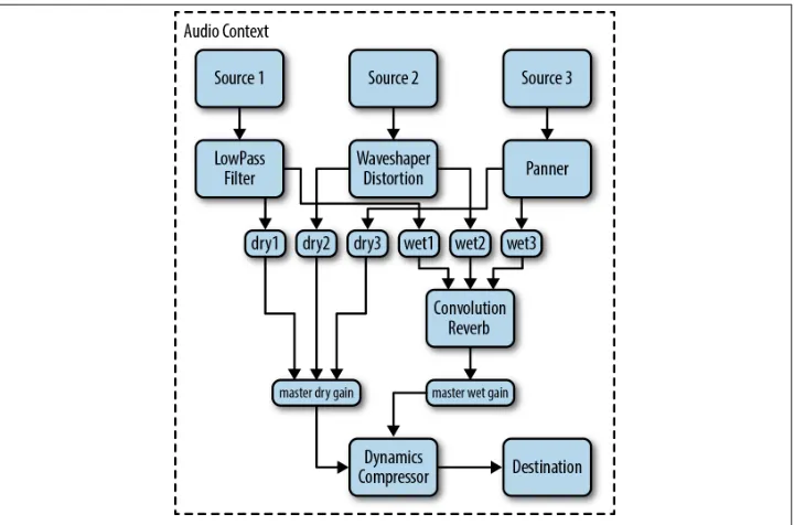
An audio context can be complex, containing many nodes between the source and destination (Figure 1-2) to perform arbitrarily advanced synthesis or analysis.
Figures 1-1 and 1-2 show audio nodes as blocks. The arrows represent connections between nodes. Nodes can often have multiple incoming and outgoing connections. By default, if there are multiple incoming connections into a node, the Web Audio API simply blends the incoming audio signals together.
The concept of an audio node graph is not new, and derives from popular audio frame‐ works such as Apple’s CoreAudio, which has an analogous Audio Processing Graph API. The idea itself is even older, originating in the 1960s with early audio environments like Moog modular synthesizer systems.
Figure 1-2. A more complex audio context
Initializing an Audio Context
The Web Audio API is currently implemented by the Chrome and Safari browsers (in‐ cluding MobileSafari as of iOS 6) and is available for web developers via JavaScript. In these browsers, the audio context constructor is webkit-prefixed, meaning that instead of creating a new AudioContext, you create a new webkitAudioContext. However, this will surely change in the future as the API stabilizes enough to ship un-prefixed and as other browser vendors implement it. Mozilla has publicly stated that they are imple‐ menting the Web Audio API in Firefox, and Opera has started participating in the working group.
With this in mind, here is a liberal way of initializing your audio context that would include other implementations (once they exist):
var contextClass = (window.AudioContext||
window.webkitAudioContext ||
window.mozAudioContext ||
window.oAudioContext ||
window.msAudioContext);
if (contextClass) {
// Web Audio API is available.
// Web Audio API is not available. Ask the user to use a supported browser.
}
A single audio context can support multiple sound inputs and complex audio graphs, so generally speaking, we will only need one for each audio application we create. The audio context instance includes many methods for creating audio nodes and manipu‐ lating global audio preferences. Luckily, these methods are not webkit-prefixed and are relatively stable. The API is still changing, though, so be aware of breaking changes (see Appendix A).
Types of Web Audio Nodes
One of the main uses of audio contexts is to create new audio nodes. Broadly speaking, there are several kinds of audio nodes:
Source nodes
Sound sources such as audio buffers, live audio inputs, <audio> tags, oscillators, and JS processors
Sources need not be based on sound files, but can instead be real-time input from a live instrument or microphone, redirection of the audio output from an audio element [see “Setting Up Background Music with the <audio> Tag” (page 53)], or entirely synthesized sound [see “Audio Processing with JavaScript” (page 51)]. Though the final destination-node is often the speakers, you can also process without sound playback (for example, if you want to do pure visualization) or do offline processing, which results in the audio stream being written to a destination buffer for later use.
Connecting the Audio Graph
Any audio node’s output can be connected to any other audio node’s input by using the connect() function. In the following example, we connect a source node’s output into a gain node, and connect the gain node’s output into the context’s destination:
// Create the source.
var source = context.createBufferSource();
// Create the gain node.
var gain = context.createGain();
// Connect source to filter, filter to destination.
source.connect(gain);
gain.connect(context.destination);
Note that context.destination is a special node that is associated with the default audio output of your system. The resulting audio graph of the previous code looks like Figure 1-3.
Figure 1-3. Our first audio graph
Once we have connected up a graph like this we can dynamically change it. We can disconnect audio nodes from the graph by calling node.disconnect(outputNumber). For example, to reroute a direct connection between source and destination, circum‐ venting the intermediate node, we can do the following:
source.disconnect(0);
gain.disconnect(0);
source.connect(context.destination);
Power of Modular Routing
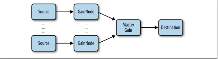
In many games, multiple sources of sound are combined to create the final mix. Sources include background music, game sound effects, UI feedback sounds, and in a multi‐ player setting, voice chat from other players. An important feature of the Web Audio API is that it lets you separate all of these different channels and gives you full control over each one, or all of them together. The audio graph for such a setup might look like Figure 1-4.
We have associated a separate gain node with each of the channels and also created a master gain node to control them all. With this setup, it is easy for your players to control the level of each channel separately, precisely the way they want to. For example, many people prefer to play games with the background music turned off.
CRITICAL THEORY
What Is Sound?
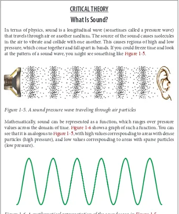
In terms of physics, sound is a longitudinal wave (sometimes called a pressure wave) that travels through air or another medium. The source of the sound causes molecules in the air to vibrate and collide with one another. This causes regions of high and low pressure, which come together and fall apart in bands. If you could freeze time and look at the pattern of a sound wave, you might see something like Figure 1-5.
Figure 1-5. A sound pressure wave traveling through air particles
Mathematically, sound can be represented as a function, which ranges over pressure values across the domain of time. Figure 1-6 shows a graph of such a function. You can see that it is analogous to Figure 1-5, with high values corresponding to areas with dense particles (high pressure), and low values corresponding to areas with sparse particles (low pressure).
Figure 1-6. A mathematical representation of the sound wave in Figure 1-5
Electronics dating back to the early twentieth century made it possible for us to capture and recreate sounds for the first time. Microphones take the pressure wave and convert
it into an electric signal, where (for example) +5 volts corresponds to the highest pressure and −5 volts to the lowest. Conversely, audio speakers take this voltage and convert it back into the pressure waves that we can hear.
Whether we are analyzing sound or synthesizing it, the interesting bits for audio pro‐ grammers are in the black box in Figure 1-7, tasked with manipulating the audio signal. In the early days of audio, this space was occupied by analog filters and other hardware that would be considered archaic by today’s standards. Today, there are modern digital equivalents for many of those old analog pieces of equipment. But before we can use software to tackle the fun stuff, we need to represent sound in a way that computers can work with.
Figure 1-7. Recording and playback
CRITICAL THEORY
What Is Digital Sound?
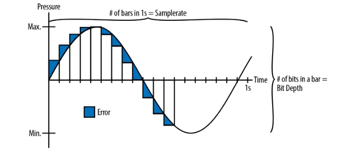
We can do this by time-sampling the analog signal at some frequency, and encoding the signal at each sample as a number. The rate at which we sample the analog signal is called the sample rate. A common sample rate in many sound applications is 44.1 kHz. This means that there are 44,100 numbers recorded for each second of sound. The numbers themselves must fall within some range. There is generally a certain number of bits allocated to each value, which is called the bit depth. For most recorded digital audio, including CDs, the bit depth is 16, which is generally enough for most listeners. Au‐ diophiles prefer 24-bit depth, which gives enough precision that people’s ears can’t hear the difference compared to a higher depth.
Figure 1-8. Analog sound being quantized, or transformed into digital sound
In Figure 1-8, the quantized digital version isn’t quite the same as the analog one because of differences between the bars and the smooth line. The difference (shown in blue) decreases with higher sample rates and bit depths. However, increasing these values also increases the amount of storage required to keep these sounds in memory, on disk, or on the Web. To save space, telephone systems often used sample rates as low as 8 kHz, since the range of frequencies needed to make the human voice intelligible is far smaller than our full audible-frequency range.
By digitizing sound, computers can treat sounds like long arrays of numbers. This sort of encoding is called pulse-code modulation (PCM). Because computers are so good at processing arrays, PCM turns out to be a very powerful primitive for most digital-audio applications. In the Web Audio API world, this long array of numbers representing a sound is abstracted as an AudioBuffer. AudioBuffers can store multiple audio channels
(often in stereo, meaning a left and right channel) represented as arrays of floating-point numbers normalized between −1 and 1. The same signal can also be represented as an array of integers, which, in 16-bit, range from (−215) to (215 − 1).
CRITICAL THEORY
Audio Encoding Formats
Raw audio in PCM format is quite large, which uses extra memory, wastes space on a hard drive, and takes up extra bandwidth when downloaded. Because of this, audio is generally stored in compressed formats. There are two kinds of compression: lossy and lossless. Lossless compression (e.g., FLAC) guarantees that when you compress and then uncompress a sound, the bits are identical. Lossy audio compression (e.g., MP3) exploits features of human hearing to save additional space by throwing out bits that we probably
won’t be able to hear anyway. Lossy formats are generally good enough for most people, with the exception of some audiophiles.
A commonly used metric for the amount of compression in audio is called bit rate, which refers to the number of bits of audio required per second of playback. The higher the bit rate, the more data that can be allocated per unit of time, and thus the less compression required. Often, lossy formats, such as MP3, are described by their bit rate (common rates are 128 and 192 Kb/s). It’s possible to encode lossy codecs at arbitrary bit rates. For example, telephone-quality human speech is often compared to 8 Kb/s MP3s. Some formats such as OGG support variable bit rates, where the bit rate changes over time. Be careful not to confuse this concept with sample rate or bit depth [see “What Is Sound?” (page 7)]!
Browser support for different audio formats varies quite a bit. Generally, if the Web Audio API is implemented in a browser, it uses the same loading code that the <au dio> tag would, so the browser support matrix for <audio> and the Web Audio API is
the same. Generally, WAV (which is a simple, lossless, and typically uncompressed for‐ mat) is supported in all browsers. MP3 is still patent-encumbered, and is therefore not available in some purely open source browsers (e.g., Firefox and Chromium). Unfortu‐ nately, the less popular but patent-unencumbered OGG format is still not available in Safari at the time of this writing.
For a more up-to-date roster of audio format support, see http://mzl.la/13kGelS.
Loading and Playing Sounds
Web Audio API makes a clear distinction between buffers and source nodes. The idea of this architecture is to decouple the audio asset from the playback state. Taking a record player analogy, buffers are like records and sources are like playheads, except in the Web Audio API world, you can play the same record on any number of playheads simulta‐ neously! Because many applications involve multiple versions of the same buffer playing simultaneously, this pattern is essential. For example, if you want multiple bouncing ball sounds to fire in quick succession, you need to load the bounce buffer only once and schedule multiple sources of playback [see “Multiple Sounds with Variations” (page 32)].
To load an audio sample into the Web Audio API, we can use an XMLHttpRequest and process the results with context.decodeAudioData. This all happens asynchronously and doesn’t block the main UI thread:
var request = new XMLHttpRequest();
request.open('GET', url, true);
request.responseType = 'arraybuffer';
context.decodeAudioData(request.response, function(theBuffer) {
buffer = theBuffer;
}, onError); }
request.send();
Audio buffers are only one possible source of playback. Other sources include direct input from a microphone or line-in device or an <audio> tag among others (see Chap‐ ter 7).
Once you’ve loaded your buffer, you can create a source node (AudioBufferSource Node) for it, connect the source node into your audio graph, and call start(0) on the source node. To stop a sound, call stop(0) on the source node. Note that both of these function calls require a time in the coordinate system of the current audio context (see Chapter 2):
function playSound(buffer) {
var source = context.createBufferSource();
source.buffer = buffer;
source.connect(context.destination);
source.start(0); }
Games often have background music playing in a loop. However, be careful about being overly repetitive with your selection: if a player is stuck in an area or level, and the same sample continuously plays in the background, it may be worthwhile to gradually fade out the track to prevent frustration. Another strategy is to have mixes of various intensity that gradually crossfade into one another depending on the game situation [see “Grad‐ ually Varying Audio Parameters” (page 16)].
Putting It All Together
As you can see from the previous code listings, there’s a bit of setup to get sounds playing in the Web Audio API. For a real game, consider implementing a JavaScript abstraction around the Web Audio API. An example of this idea is the following BufferLoader class. It puts everything together into a simple loader, which, given a set of paths, returns a set of audio buffers. Here’s how such a class can be used:
window.onload = init;
var context;
var bufferLoader;
function init() {
context = new webkitAudioContext();
bufferLoader = new BufferLoader(
context,
[
'../sounds/hyper-reality/br-jam-loop.wav',
'../sounds/hyper-reality/laughter.wav',
],
finishedLoading
);
bufferLoader.load(); }
function finishedLoading(bufferList) {
// Create two sources and play them both together.
var source1 = context.createBufferSource();
var source2 = context.createBufferSource();
source1.buffer = bufferList[0];
source2.buffer = bufferList[1];
source1.connect(context.destination);
source2.connect(context.destination);
source1.start(0);
source2.start(0); }
CHAPTER 2
Perfect Timing and Latency
One of the strengths of the Web Audio API as compared to the <audio> tag is that it comes with a low-latency precise-timing model.
Low latency is very important for games and other interactive applications since you often need fast auditory response to user actions. If the feedback is not immediate, the user will sense the delay, which will lead to frustration. In practice, due to imperfections of human hearing, there is leeway for a delay of up to 20 ms or so, but the number varies depending on many factors.
Precise timing enables you to schedule events at specific times in the future. This is very important for scripted scenes and musical applications.
Timing Model
One of the key things that the audio context provides is a consistent timing model and frame of reference for time. Importantly, this model is different from the one used for JavaScript timers such as setTimeout, setInterval, and new Date(). It is also different from the performance clock provided by window.performance.now().
All of the absolute times that you will be dealing with in the Web Audio API are in seconds (not milliseconds!), in the coordinate system of the specified audio context. The current time can be retrieved from the audio context via the currentTime property. Although the units are seconds, time is stored as a floating-point value with high pre‐ cision.
Precise Playback and Resume
The start() function makes it easy to schedule precise sound playback for games and other time-critical applications. To get this working properly, ensure that your sound buffers are pre-loaded [see “Loading and Playing Sounds” (page 10)]. Without a
pre-loaded buffer, you will have to wait an unknown amount of time for the browser to fetch the sound file, and then for the Web Audio API to decode it. The failure mode in this case is you want to play a sound at a precise instant, but the buffer is still loading or decoding.
Sounds can be scheduled to play at a precise time by specifying the first (when) parameter of the start() call. This parameter is in the coordinate system of the AudioContext’s currentTime. If the parameter is less than the currentTime, it is played immediately. Thus start(0) always plays sound immediately, but to schedule sound in 5 seconds, you would call start(context.currentTime + 5).
Sound buffers can also be played from a specific time offset by specifying a second parameter to the start() call, and limited to a specific duration with a third optional parameter. For example, if we want to pause a sound and play it back from the paused position, we can implement a pause by tracking the amount of time a sound has been playing in the current session and also tracking the last offset in order to resume later:
// Assume context is a web audio context, buffer is a pre-loaded audio buffer. var startOffset = 0;
var startTime = 0;
function pause() {
source.stop();
// Measure how much time passed since the last pause.
startOffset += context.currentTime - startTime; }
Once a source node has finished playing back, it can’t play back more. To play back the underlying buffer again, you need to create a new source node (AudioBufferSource Node) and call start():
function play() {
startTime = context.currentTime;
var source = context.createBufferSource();
// Connect graph
source.buffer = this.buffer;
source.loop = true;
source.connect(context.destination);
// Start playback, but make sure we stay in bound of the buffer.
source.start(0, startOffset % buffer.duration); }
Scheduling Precise Rhythms
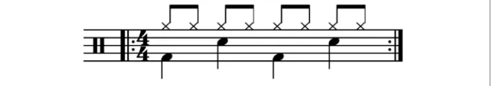
The Web Audio API lets developers precisely schedule playback in the future. To demonstrate this, let’s set up a simple rhythm track. Probably the simplest and most widely known drumkit pattern is shown in Figure 2-1, in which a hihat is played every eighth note, and the kick and snare are played on alternating quarter notes, in 4/4 time.
Figure 2-1. Sheet music for one of the most basic drum patterns
Assuming we have already loaded the kick, snare, and hihat buffers, the code to do this is simple:
for (var bar = 0; bar < 2; bar++) {
var time = startTime + bar * 8 * eighthNoteTime;
// Play the bass (kick) drum on beats 1, 5
playSound(kick, time);
playSound(kick, time + 4 * eighthNoteTime);
// Play the snare drum on beats 3, 7
playSound(snare, time + 2 * eighthNoteTime);
playSound(snare, time + 6 * eighthNoteTime);
// Play the hihat every eighth note.
for (var i = 0; i < 8; ++i) {
playSound(hihat, time + i * eighthNoteTime);
} }
Once you’ve scheduled sound in the future, there is no way to unschedule that future playback event, so if you are dealing with an application that quickly changes, scheduling sounds too far into the future is not advisable. A good way of dealing with this problem is to create your own scheduler using JavaScript timers and an event queue. This ap‐ proach is described in A Tale of Two Clocks.
Demo: to see this code in action, visit http://webaudioapi.com/samples/rhythm/.
Changing Audio Parameters
Many types of audio nodes have configurable parameters. For example, the GainNode has a gain parameter that controls the gain multiplier for all sounds going through the
node. Specifically, a gain of 1 does not affect the amplitude, 0.5 halves it, and 2 doubles it [see “Volume, Gain, and Loudness” (page 21)]. Let’s set up a graph as follows:
// Create a gain node.
var gainNode = context.createGain();
// Connect the source to the gain node. source.connect(gainNode);
// Connect the gain node to the destination. gainNode.connect(context.destination);
In the context of the API, audio parameters are represented as AudioParam instances. The values of these nodes can be changed directly by setting the value attribute of a param instance:
// Reduce the volume. gainNode.gain.value = 0.5;
The values can also be changed later, via precisely scheduled parameter changes in the future. We could also use setTimeout to do this scheduling, but this is not precise for several reasons:
1. Millisecond-based timing may not be enough precision.
2. The main JS thread may be busy with high-priority tasks like page layout, garbage collection, and callbacks from other APIs, which delays timers.
3. The JS timer is affected by tab state. For example, interval timers in backgrounded tabs fire more slowly than if the tab is in the foreground.
Instead of setting the value directly, we can call the setValueAtTime() function, which takes a value and a start time as arguments. For example, the following snippet sets the gain value of a GainNode in one second:
gainNode.gain.setValueAtTime(0.5, context.currentTime + 1);
Demo: for a simple example of changing the gain parameter, visit http://webaudioa pi.com/samples/volume/.
Gradually Varying Audio Parameters
In many cases, rather than changing a parameter abruptly, you would prefer a more gradual change. For example, when building a music player application, we want to fade the current track out, and fade the new one in, to avoid a jarring transition. While you can achieve this with multiple calls to setValueAtTime as described previously, this is inconvenient.
way the transition happens. In some cases, an exponential transition makes more sense, since we perceive many aspects of sound in an exponential manner.
Let’s take an example of scheduling a crossfade in the future. Given a playlist, we can transition between tracks by scheduling a gain decrease on the currently playing track, and a gain increase on the next one, both slightly before the current track finishes playing:
function createSource(buffer) {
var source = context.createBufferSource();
var gainNode = context.createGainNode();
source.buffer = buffer;
// Connect source to gain.
source.connect(gainNode);
// Connect gain to destination.
gainNode.connect(context.destination);
return {
source: source,
gainNode: gainNode
}; }
function playHelper(buffers, iterations, fadeTime) {
var currTime = context.currentTime;
Demo: to see this code in action, visit http://webaudioapi.com/samples/crossfade-playlist/.
Custom Timing Curves
If neither a linear nor an exponential curve satisfies your needs, you can also specify your own value curve via an array of values using the setValueCurveAtTime function. With this function, you can define a custom timing curve by providing an array of timing values. It’s a shortcut for making a bunch of setValueAtTime calls, and should be used in this case. For example, if we want to create a tremolo effect, we can apply an oscillating curve to the gain AudioParam of a GainNode, as in Figure 2-2.
Figure 2-2. A value curve oscillating over time
The oscillating curve in the previous figure could be implemented with the following code:
var DURATION = 2;
var FREQUENCY = 1;
var SCALE = 0.4;
// Split the time into valueCount discrete steps. var valueCount = 4096;
// Create a sinusoidal value curve. var values = new Float32Array(valueCount);
for (var i = 0; i < valueCount; i++) {
var percent = (i / valueCount) * DURATION*FREQUENCY;
values[i] = 1 + (Math.sin(percent * 2*Math.PI) * SCALE);
// Set the last value to one, to restore playbackRate to normal at the end.
if (i == valueCount - 1) {
values[i] = 1;
} }
// Apply it to the gain node immediately, and make it last for 2 seconds. this.gainNode.gain.setValueCurveAtTime(values, context.currentTime, DURATION);
This brings us to a very nifty feature of the Web Audio API that lets us build effects like tremolo more easily. We can take any audio stream that would ordinarily be connected into another AudioNode, and instead connect it into any AudioParam. This important idea is the basis for many sound effects. The previous code is actually an example of such an effect called a low frequency oscillator (LFO) applied to the gain, which is used to build effects such as vibrato, phasing, and tremolo. By using the oscillator node [see “Oscillator-Based Direct Sound Synthesis” (page 34)], we can easily rebuild the previous example as follows:
// Create oscillator.
var osc = context.createOscillator();
osc.frequency.value = FREQUENCY;
var gain = context.createGain();
gain.gain.value = SCALE;
osc.connect(gain);
gain.connect(this.gainNode.gain);
// Start immediately, and stop in 2 seconds. osc.start(0);
osc.stop(context.currentTime + DURATION);
The latter approach is more efficient than creating a custom value curve and saves us from having to compute sine functions manually by creating a loop to repeat the effect.
CHAPTER 3
Volume and Loudness
Once we are ready to play a sound, whether from an AudioBuffer or from other sources, one of the most basic parameters we can change is the loudness of the sound.
The main way to affect the loudness of a sound is using GainNodes. As previously men‐ tioned, these nodes have a gain parameter, which acts as a multiplier on the incoming sound buffer. The default gain value is one, which means that the input sound is unaf‐ fected. Values between zero and one reduce the loudness, and values greater than one amplify the loudness. Negative gain (values less than zero) inverts the waveform (i.e., the amplitude is flipped).
CRITICAL THEORY
Volume, Gain, and Loudness
Let’s start with some definitions. Loudness is a subjective measure of how intensely our ears perceive a sound. Volume is a measure of the physical amplitude of a sound wave. Gain is a scale multiplier affecting a sound’s amplitude as it is being processed.
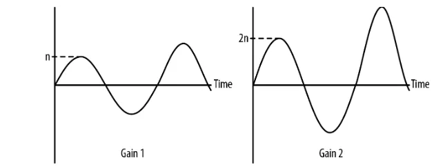
In other words, when undergoing a gain, the amplitude of a sound wave is scaled, with the gain value used as a multiplier. For example, while a gain value of one will not affect the sound wave at all, Figure 3-1 illustrates what happens to a sound wave if you send it through a gain factor of two.
Figure 3-1. Original soundform on the left, gain 2 soundform on the right
Generally speaking, power in a wave is measured in decibels (abbreviated dB), or one tenth of a Bel, named after Alexander Graham Bell. Decibels are a relative, logarithmic unit that compare the level being measured to some reference point. There are many different reference points for measuring dB, and each reference point is indicated with a suffix on the unit. Saying that a signal is some number of dB is meaningless without a reference point! For example, dBV, dBu, and dBm are all useful for measuring electrical signals. Since we are dealing with digital audio, we are mainly concerned with two measures: dBFS and dBSPL.
The first is dBFS, or decibels full scale. The highest possible level of sound produced by audio equipment is 0 dBFS. All other levels are expressed in negative numbers. dBFS is described mathematically as:
dBFS = 20 * log( [sample level] / [max level] )
The maximum dBFS value in a 16-bit audio system is:
max = 20 * log(1111 1111 11111111/1111 1111 1111 1111) = log(1) = 0
Note that the maximum dBFS value will always be 0 by definition, since log(1) = 0. Similarly, the minimum dBFS value in the same system is:
min = 20 * log(0000 0000 00000001/1111 1111 1111 1111) = -96 dBFS
The logarithmic definition of decibels correlates somewhat to the way our ears perceive loudness, but loudness is still a very subjective concept. Comparing the dB values of a sound and the same sound with a 2x gain, we can see that we’ve gained about 6 dB:
diff = 20 * log(2/2^16) - 20 * log(1/2^16) = 6.02 dB
Every time we add 6 dB or so, we actually double the amplitude of the signal. Comparing the sound at a rock concert (~110 dBSPL) to your alarm clock (~80 dBSPL), the differ‐ ence between the two is (110 − 80)/6 dB, or roughly 5 times louder, with a gain multiplier of 25 = 32x. A volume knob on a stereo is therefore also calibrated to increase the am‐ plitude exponentially. In other words, turning the volume knob by 3 units multiplies the amplitude of the signal roughly by a factor of 23 or 8 times. In practice, the expo‐ nential model described here is merely an approximation to the way our ears perceive loudness, and audio equipment manufacturers often have their own custom gain curves that are neither linear nor exponential.
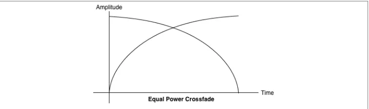
Equal Power Crossfading
Often in a game setting, you have a situation where you want to crossfade between two environments that have different sounds associated with them. However, when to crossfade and by how much is not known in advance; perhaps it varies with the position of the game avatar, which is controlled by the player. In this case, we cannot do an automatic ramp.
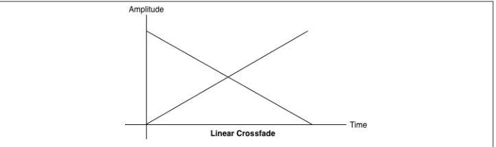
In general, doing a straightforward, linear fade will result in the following graph. It can sound unbalanced because of a volume dip between the two samples, as shown in Figure 3-2.
Figure 3-2. A linear crossfade between two tracks
To address this issue, we use an equal power curve, in which the corresponding gain curves are neither linear nor exponential, and intersect at a higher amplitude (Figure 3-3). This helps avoid a dip in volume in the middle part of the crossfade, when both sounds are mixed together equally.
Figure 3-3. An equal power crossfade sounds much better
The graph in Figure 3-3 can be generated with a bit of math: function equalPowerCrossfade(percent) {
// Use an equal-power crossfading curve:
var gain1 = Math.cos(percent * 0.5*Math.PI);
var gain2 = Math.cos((1.0 - percent) * 0.5*Math.PI);
this.ctl1.gainNode.gain.value = gain1;
this.ctl2.gainNode.gain.value = gain2; }
Demo: to listen to an equal power crossfade, visit http://webaudioapi.com/samples/cross fade/.
CRITICAL THEORY
Clipping and Metering
Figure 3-4. A meter in a typical receiver
Clipped sound looks bad on a monitor and sounds no better. It’s important to listen for harsh distortions, or conversely, overly subdued mixes that force your listeners to crank up the volume. If you’re in either of these situations, read on!
Using Meters to Detect and Prevent Clipping
Since multiple sounds playing simultaneously are additive with no level reduction, you may find yourself in a situation where you are exceeding past the threshold of your speaker’s capability. The maximum level of sound is 0 dBFS, or 216, for 16-bit audio. In the floating point version of the signal, these bit values are mapped to [−1, 1]. The waveform of a sound that’s being clipped looks something like Figure 3-5. In the context of the Web Audio API, sounds clip if the values sent to the destination node lie outside of the range. It’s a good idea to leave some room (called headroom) in your final mix so that you aren’t too close to the clipping threshold.
Figure 3-5. A diagram of a waveform being clipped
In addition to close listening, you can check whether or not you are clipping your sound programmatically by putting a script processor node into your audio graph. Clipping may occur if any of the PCM values are out of the acceptable range. In this sample, we check both left and right channels for clipping, and if clipping is detected, save the last clipping time:
function onProcess(e) {
var leftBuffer = e.inputBuffer.getChannelData(0);
var rightBuffer = e.inputBuffer.getChannelData(1);
checkClipping(leftBuffer);
checkClipping(rightBuffer); }
function checkClipping(buffer) {
var isClipping = false;
// Iterate through buffer to check if any of the |values| exceeds 1.
for (var i = 0; i < buffer.length; i++) {
An alternative implementation of metering could poll a real-time analyzer in the audio graph for getFloatFrequencyData at render time, as determined by requestAnima tionFrame (see Chapter 5). This approach is more efficient, but misses a lot of the signal (including places where it potentially clips), since rendering happens most at 60 times a second, whereas the audio signal changes far more quickly.
Demo: for an example of a very simple meter, visit http://webaudioapi.com/samples/ metering/.
CRITICAL THEORY
Understanding Dynamic Range
In audio, dynamic range refers to the difference between the loudest and quietest parts of a sound. The amount of dynamic range in musical pieces varies greatly depending on genre. Classical music has large dynamic range and often features very quiet sections followed by relatively loud ones. Many popular genres like rock and electronica tend to have a small dynamic range, and are uniformly loud because of an apparent competition (known pejoratively as the “Loudness War”) to increase the loudness of tracks to meet consumer demands. This uniform loudness is generally achieved by using dynamic range compression.
That said, there are many legitimate uses of compression. Sometimes recorded music has such a large dynamic range that there are sections that sound so quiet or loud that the listener constantly needs to have a finger on the volume knob. Compression can quiet down the loud parts while making the quiet parts audible. Figure 3-6 illustrates a waveform (above), and then the same waveform with compression applied (below). You can see that the sound is louder overall, and there is less variance in the amplitude.
Figure 3-6. The effects of dynamics compression
For games and interactive applications, you may not know beforehand what your sound output will look like. Because of games’ dynamic nature, you may have very quiet periods (e.g., stealthy sneaking) followed by very loud ones (e.g., a warzone). A compressor node can be helpful in suddenly loud situations for reducing the likelihood of clipping [see “Clipping and Metering” (page 24)].
Compressors can be modeled with a compression curve with several parameters, all of which can be tweaked with the Web Audio API. Two of the main parameters of a
compressor are threshold and ratio. Threshold refers to the lowest volume at which a compressor starts reducing dynamic range. Ratio determines how much gain reduction is applied by the compressor. Figure 3-7 illustrates the effect of threshold and various compression ratios on the compression curve.
Figure 3-7. A sample compression curve with basic parameters
Dynamics Compression
Compressors are available in the Web Audio API as DynamicsCompressorNodes. Using moderate amounts of dynamics compression in your mix is generally a good idea, es‐ pecially in a game setting where, as previously discussed, you don’t know exactly what sounds will play and when. One case where compression should be avoided is when dealing with painstakingly mastered tracks that have been tuned to sound “just right” already, which are not being mixed with any other tracks.
Implementing dynamic compression in the Web Audio API is simply a matter of in‐ cluding a dynamics compressor node in your audio graph, generally as the last node before the destination:
var compressor = context.createDynamicsCompressor();
mix.connect(compressor);
compressor.connect(context.destination);
CHAPTER 4
Pitch and the Frequency Domain
So far we have learned about some basic properties of sound: timing and volume. To do more complex things, such as sound equalization (e.g., increasing the bass and de‐ creasing the treble), we need more complex tools. This section explains some of the tools that allow you to do these more interesting transformations, which include the ability to simulate different sorts of environments and manipulate sounds directly with JavaScript.
CRITICAL THEORY
Basics of Musical Pitch
Music consists of many sounds played simultaneously. Sounds produced by musical instruments can be very complex, as the sound bounces through various parts of the instrument and is shaped in unique ways. However, these musical tones all have one thing in common: physically, they are periodic waveforms. This periodicity is perceived by our ears as pitch. The pitch of a note is measured in frequency, or the number of times the wave pattern repeats every second, specified in hertz. The frequency is the time (in seconds) between the crests of the wave. As illustrated in Figure 4-1, if we halve the wave in the time dimension, we end up with a correspondingly doubled frequency, which sounds to our ears like the same tone, one octave higher. Conversely, if we extend the wave’s frequency by two, this brings the tone an octave down. Thus, pitch (like volume) is perceived exponentially by our ears: at every octave, the frequency doubles.
Figure 4-1. Graph of perfect A4 and A5 tones side by side
Octaves are split up into 12 semitones. Each adjacent semitone pair has an identical frequency ratio (at least in equal-tempered tunings). In other words, the ratios of the frequencies of A4 to A#4 are identical to A#4 to B.
Figure 4-1 shows how we would derive the ratio between every successive semitone, given that:
1. To transpose a note up an octave, we double the frequency of the note.
2. Each octave is split up into 12 semitones, which, in an equal tempered tuning, have identical frequency ratios.
Let’s define a f0 to be some frequency, and f1 to be that same note one octave higher.
we know that this is the relationship between them:
f1= 2 *f0
Next, let k be the fixed multiplier between any two adjacent semitones. Since there are 12 semitones in an octave, we also know the following:
f1= f0*k*k*k* ... *k(12x) = f0*k12
Solving the system of equations above, we have the following:
2 *f0= f0*k12
Solving for k:
Conveniently, all of this semitone-related offsetting isn’t really necessary to do manually, since many audio environments (the Web Audio API included) include a notion of detune, which linearizes the frequency domain. Detune is measured in cents, with each octave consisting of 1200 cents, and each semitone consisting of 100 cents. By specifying a detune of 1200, you move up an octave. Specifying a detune of −1200 moves you down an octave.
Pitch and playbackRate
The Web Audio API provides a playbackRate parameter on each AudioSourceNode. This value can be set to affect the pitch of any sound buffer. Note that the pitch as well as the duration of the sample will be affected in this case. There are sophisticated meth‐ ods that try to affect pitch independent of duration, but this is quite difficult to do in a general-purpose way without introducing blips, scratches, and other undesirable arti‐ facts to the mix.
As discussed in “Basics of Musical Pitch” (page 29), to compute the frequencies of suc‐ cessive semitones, we simply multiply the frequency by the semitone ratio 21/12. This is very useful if you are developing a musical instrument or using pitch for randomization in a game setting. The following code plays a tone at a given frequency offset in semitones:
function playNote(semitones) {
// Assume a new source was created from a buffer.
var semitoneRatio = Math.pow(2, 1/12);
source.playbackRate.value = Math.pow(semitoneRatio, semitones);
source.start(0); }
As we discussed earlier, our ears perceive pitch exponentially. Treating pitch as an ex‐ ponential quantity can be inconvenient, since we often deal with awkward values such as the twelfth root of two. Instead of doing that, we can use the detune parameter to specify our offset in cents. Thus you can rewrite the above function using detune in an easier way:
If you pitch shift by too many semitones (e.g., by calling playNote(24);), you will start to hear distortions. Because of this, digital pianos include multiple samples for each instrument. Good digital pianos avoid pitch bending at all, and include a separate sample recorded specifically for each key. Great digital pianos often include multiple samples for each key, which are played back depending on the velocity of the key press.
Multiple Sounds with Variations
A key feature of sound effects in games is that there can be many of them simultaneously. Imagine you’re in the middle of a gunfight with multiple actors shooting machine guns. Each machine gun fires many times per second, causing tens of sound effects to be played at the same time. Playing back sound from multiple, precisely-timed sources simultaneously is one place the Web Audio API really shines.
Now, if all of the machine guns in your game sounded exactly the same, that would be pretty boring. Of course the sound would vary based on distance from the target and relative position [more on this later in “Spatialized Sound” (page 49)], but even that might not be enough. Luckily the Web Audio API provides a way to easily tweak the previous example in at least two simple ways:
1. With a subtle shift in time between bullets firing
2. By changing pitch to better simulate the randomness of the real world
Using our knowledge of timing and pitch, implementing these two effects is pretty straightforward:
function shootRound(numberOfRounds, timeBetweenRounds) {
var time = context.currentTime;
// Make multiple sources using the same buffer and play in quick succession.
for (var i = 0; i < numberOfRounds; i++) {
The Web Audio API automatically merges multiple sounds playing at once, essentially just adding the waveforms together. This can cause problems such as clipping, which we discuss in “Clipping and Metering” (page 24).
This example adds some variety to AudioBuffers loaded from sound files. In some cases, it is desirable to have fully synthesized sound effects and no buffers at all [see “Procedurally Generated Sound” (page 45)].
Demo: to hear multiple gunshot samples played in rapid succession, visit http://webau dioapi.com/samples/rapid-sounds/.
CRITICAL THEORY
Understanding the Frequency Domain
see how it varies over frequency. This results in graphs where the domain (x-axis) is in units of frequency (Hz). Graphs of sound plotted this way are said to be in the frequency domain.
The relationship between the time-domain and frequency-domain graphs is based on the idea of fourier decomposition. As we saw earlier, sound waves are often cyclical in nature. Mathematically, periodic sound waves can be seen as the sum of multiple simple sine waves of different frequency and amplitude. The more such sine waves we add together, the better an approximation of the original function we can get. We can take a signal and find its component sine waves by applying a fourier transformation, the details of which are outside the scope of this book. Many algorithms exist to get this decomposition too, the best known of which is the Fast Fourier Transform (FFT). Luck‐ ily, the Web Audio API comes with an implementation of this algorithm. We will discuss how it works later [see “Frequency Analysis” (page 37)].
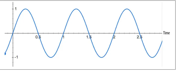
In general, we can take a sound wave, figure out the constituent sine wave breakdown, and plot the (frequency, amplitude) as points on a new graph to get a frequency domain plot. Figure 4-2 shows a pure A note at 440 Hz (called A4).
Figure 4-2. A perfectly sinusoidal 1-KHz sound wave represented in both time and frequency domains
Looking at the frequency domain can give a better sense of the qualities of the sound, including pitch content, amount of noise, and much more. Advanced algorithms like pitch detection can be built on top of the frequency domain. Sound produced by real musical instruments have overtones, so an A4 played by a piano has a frequency domain plot that looks (and sounds) very different from the same A4 pitch played by a trumpet.
Regardless of the complexity of sounds, the same fourier decomposition ideas apply. Figure 4-3 shows a more complex fragment of a sound in both the time and frequency domains.
Figure 4-3. A complex sound wave shown in both time and frequency domains
These graphs behave quite differently over time. If you were to very slowly play back the sound in Figure 4-3 and observe it moving along each graph, you would notice the time domain graph (on the left) progressing left to right. The frequency domain graph (on the right) is the frequency analysis of the waveform at a moment in time, so it might change more quickly and less predictably.
Importantly, frequency-domain analysis is still useful when the sound examined is not perceived as having a specific pitch. Wind, percussive sources, and gunshots have dis‐ tinct representations in the frequency domain. For example, white noise has a flat fre‐ quency domain spectrum, since each frequency is equally represented.
Oscillator-Based Direct Sound Synthesis
As we discussed early in this book, digital sound in the Web Audio API is represented as an array of floats in AudioBuffers. Most of the time, the buffer is created by loading a sound file, or on the fly from some sound stream. In some cases, we might want to synthesize our own sounds. We can do this by creating audio buffers programmatically using JavaScript, which simply evaluate a mathematical function at regular periods and assign values to an array. By taking this approach, we can manually change the amplitude and frequency of our sine wave, or even concatenate multiple sine waves together to create arbitrary sounds [recall the principles of fourier transformations from “Under‐ standing the Frequency Domain” (page 32)].
Pitch” (page 29)]. They also have a type that represents the kind of wave to generate. Built-in types include the sine, triangle, sawtooth, and square waves, as shown in Figure 4-4.
Figure 4-4. Types of basic soundwave shapes that the oscillator can generate
Oscillators can easily be used in audio graphs in place of AudioBufferSourceNodes. An example of this follows:
function play(semitone) {
// Create some sweet sweet nodes.
var oscillator = context.createOscillator();
oscillator.connect(context.destination);
// Play a sine type curve at A4 frequency (440hz).
oscillator.frequency.value = 440;
oscillator.detune.value = semitone * 100;
// Note: this constant will be replaced with "sine".
oscillator.type = oscillator.SINE;
oscillator.start(0); }
Demo: to listen to oscillators of various types, visit http://webaudioapi.com/samples/oscil lator/.
In addition to these basic wave types, you can create a custom wave table for your oscillator by using harmonic tables. This lets you efficiently create wave shapes that are much more complex than the previous ones. This topic is very important for musical synthesis applications, but is outside of the scope of this book.
CHAPTER 5
Analysis and Visualization
So far we’ve only talked about audio synthesis and processing, but that is only half of the functionality that the Web Audio API provides. The other half, audio analysis, is all about understanding what the sound that is being played is like. The canonical example of this feature is visualization, but there are many other applications far outside the scope of this book, including pitch detection, rhythm detection, and speech recognition. This is an important topic for us as game developers and interactive application builders for a couple of reasons. Firstly, a good visual analyzer can act as a sort of debugging tool (obviously in addition to your ears and a good metering setup) for tweaking sounds to be just right. Secondly, visualization is critical for any games and applications related to music, from games like Guitar Hero to software like GarageBand.
Frequency Analysis
The main way of doing sound analysis with the Web Audio API is to use AnalyserNo des. These nodes do not change the sound in any way, and can be placed anywhere in your audio context. Once this node is in your graph, it provides two main ways for you to inspect the sound wave: over the time domain and over the frequency domain. The results you get are based on FFT analysis over a certain buffer size. We have a few knobs to customize the output of the node:
fftSize
This defines the buffer size that is used to perform the analysis. It must be a power of two. Higher values will result in more fine-grained analysis of the signal, at the cost of some performance loss.
frequencyBinCount
This is a read-only property, set automatically as fftSize/2.
smoothingTimeConstant
This is a value between zero and one. A value of one causes a large moving average window and smoothed results. A value of zero means no moving average, and quickly fluctuating results.
The basic setup is to insert the analyzer node into the interesting part of our audio graph: // Assume that node A is ordinarily connected to B.
var analyser = context.createAnalyser();
A.connect(analyser);
analyser.connect(B);
Then we can get frequency or time domain arrays as follows: var freqDomain = new Float32Array(analyser.frequencyBinCount);
analyser.getFloatFrequencyData(freqDomain);
In the previous example, freqDomain is an array of 32-bit floats corresponding to the frequency domain. These values are normalized to be between zero and one. The indexes of the output can be mapped linearly between zero and the nyquist frequency, which is defined to be half of the sampling rate (available in the Web Audio API via con text.sampleRate). The following snippet maps from frequency to the correct bucket in the array of frequencies:
function getFrequencyValue(frequency) {
var nyquist = context.sampleRate/2;
var index = Math.round(frequency/nyquist * freqDomain.length);
return freqDomain[index]; }
If we are analyzing a 1,000-Hz sine wave, for example, we would expect that getFre quencyValue(1000) would return a peak value in the graph, as shown in Figure 5-1.
Figure 5-1. A 1,000-Hz tone being visualized (the full domain extends from 0 to 22,050 Hz)
Animating with requestAnimationFrame
If we want to build a visualization for our soundform, we need to periodically query the analyzer, process the results, and render them. We can do this by setting up a JavaScript timer like setInterval or setTimeout, but there’s a better way: requestAnimation Frame. This API lets the browser incorporate your custom draw function into its native rendering loop, which is a great performance improvement. Instead of forcing it to draw at specific intervals and contending with the rest of the things a browser does, you just request it to be placed in the queue, and the browser will get to it as quickly as it can. Because the requestAnimationFrame API is still experimental, we need to use the pre‐ fixed version depending on user agent, and fall back to a rough equivalent: setTime out. The code for this is as follows:
window.requestAnimationFrame = (function(){
return window.requestAnimationFrame ||
window.webkitRequestAnimationFrame ||
window.mozRequestAnimationFrame ||
window.oRequestAnimationFrame ||
window.msRequestAnimationFrame ||
function(callback){
window.setTimeout(callback, 1000 / 60); };
})();
Once we have this requestAnimationFrame function defined, we should use it to query the analyzer node to give us detailed information about the state of the audio stream.