Introduction to Finite Elements CVEN45255525

Draft

DRAFT

Lecture Notes in:

MATRIX STRUCTURAL ANALYSIS

with an

Introduction to Finite Elements

CVEN4525/5525

c

VICTOR E. SAOUMA,

Fall 1999

Draft

Contents

1 INTRODUCTION

1–1

1.1

Why Matrix Structural Analysis? . . . 1–1

1.2

Overview of Structural Analysis . . . 1–2

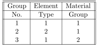
1.3 Structural Idealization . . . 1–4

1.3 .1

Structural Discretization . . . 1–5

1.3 .2

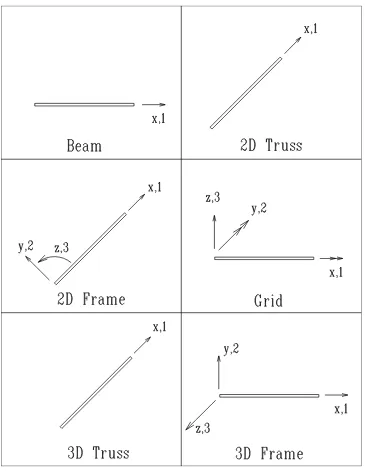
Coordinate Systems . . . 1–6

1.3 .3

Sign Convention . . . 1–6

1.4

Degrees of Freedom . . . 1–9

1.5

Course Organization . . . 1–11

I

Matrix Structural Analysis of Framed Structures

1–15

2 ELEMENT STIFFNESS MATRIX

2–1

3 .1

Introduction . . . 3 –1

3 .2

The Stiffness Method . . . 3 –2

3 .3

Examples . . . 3 –4

E 3 -1 Beam . . . 3 –4

E 3 -2 Frame . . . 3 –6

E 3 -3

Grid . . . 3 –9

3 .4

Observations . . . 3 –13

4 TRANSFORMATION MATRICES

4–1

4.1

Derivations . . . 4–1

4.1.1

[

k

e

_{] [}

_K

e

_{] Relation}

_{. . . 4–1}

4.1.2

Direction Cosines . . . 4–2

4.2

Transformation Matrices For Framework Elements . . . 4–6

4.2.1

2 D cases . . . 4–6

4.2.1.1

2D Frame, and Grid Element . . . 4–6

4.2.1.2

2D Truss . . . 4–8

4.2.2

3 D Frame . . . 4–8

4.2.2.1

Simple 3 D Case . . . 4–9

4.2.2.2

General Case . . . 4–12

4.2.3 3

D Truss . . . 4–15

5 STIFFNESS METHOD; Part II

5–1

Draft

CONTENTS

0–3

5.8.1.1

Input Variable Descriptions . . . 5–3 7

5.8.1.2

Sample Input Data File . . . 5–3 8

5.8.1.3 Program Implementation . . . 5–40

5.8.2

Program Listing . . . 5–40

5.8.2.1

Main Program . . . 5–40

5.8.2.2

Assembly of

ID

Matrix . . . 5–43

5.8.2.3 Element Nodal Coordinates . . . 5–44

5.8.2.4

Element Lengths . . . 5–45

5.8.2.5

Element Stiffness Matrices . . . 5–45

5.8.2.6

Transformation Matrices . . . 5–46

5.8.2.7

Assembly of the Augmented Stiffness Matrix . . . 5–47

5.8.2.8

Print General Information . . . 5–48

5.8.2.9

Print Load . . . 5–49

5.8.2.10 Load Vector . . . 5–50

5.8.2.11 Nodal Displacements . . . 5–52

5.8.2.12 Reactions . . . 5–53

5.8.2.13 Internal Forces . . . 5–54

5.8.2.14 Sample Output File . . . 5–55

6 EQUATIONS OFSTATICS and KINEMATICS

6–1

6.1

Statics Matrix [

_B

] . . . 6–1

E 6-1 Statically Determinate Truss Statics Matrix . . . 6–2

E 6-2 Beam Statics Matrix . . . 6–4

E 6-3 Statically Indeterminate Truss Statics Matrix . . . 6–6

6.1.1

Identification of Redundant Forces . . . 6–9

E 6-4 Selection of Redundant Forces

. . . 6–9

6.1.2

Kinematic Instability . . . 6–12

6.2

Kinematics Matrix [

_A

] . . . 6–12

E 6-5 Kinematics Matrix of a Truss . . . 6–14

6.3 Statics-Kinematics Matrix Relationship . . . 6–15

6.3 .1

Statically Determinate . . . 6–15

6.3 .2

Statically Indeterminate . . . 6–16

6.4

Kinematic Relations through Inverse of Statics Matrix . . . 6–16

6.5

Congruent Transformation Approach to [

K

] . . . 6–17

E 6-6 Congruent Transformation . . . 6–18

E 6-7 Congruent Transformation of a Frame . . . 6–20

7 FLEXIBILITY METHOD

7–1

7.3Stiffness Flexibility Relations . . . 7–5

7.3.1

From Stiffness to Flexibility . . . 7–6

E 7-2 Flexibility Matrix

. . . 7–6

7.3.2

From Flexibility to Stiffness . . . 7–7

E 7-3Flexibility to Stiffness . . . 7–8

7.4

Stiffness Matrix of a Curved Element . . . 7–9

7.5

Duality between the Flexibility and the Stiffness Methods . . . 7–11

II

Introduction to Finite Elements

7–13

8 REVIEW OFELASTICITY

8–1

8.1

Stress . . . 8–1

8.1.1

Stress Traction Relation . . . 8–2

8.2

Strain . . . 8–3

8.3Fundamental Relations in Elasticity . . . 8–4

8.3.1

Equation of Equilibrium . . . 8–4

8.3.2

Compatibility Equation . . . 8–5

8.4

Stress-Strain Relations in Elasticity . . . 8–6

8.5

Strain Energy Density . . . 8–7

8.6

Summary . . . 8–7

9 VARIATIONAL AND ENERGY METHODS

9–1

Draft

CONTENTS

0–5

9.2.5.1.2

Linear Elastic Systems . . . 9–17

9.2.5.2

External Complementary Virtual Work

δW

∗

. . . 9–18

9.2.6

Potential Energy . . . 9–18

9.2.6.1

Potential Functions . . . 9–18

9.2.6.2

Potential of External Work . . . 9–19

9.2.6.3 Potential Energy . . . 9–19

9.3 Principle of Virtual Work and Complementary Virtual Work . . . 9–19

9.3 .1

Principle of Virtual Work . . . 9–20

9.3.1.1

_†

Derivation . . . 9–20

E 9-3Tapered Cantiliver Beam, Virtual Displacement . . . 9–23

9.3 .2

Principle of Complementary Virtual Work . . . 9–25

9.3.2.1

_†

Derivation . . . 9–25

E 9-4 Tapered Cantilivered Beam; Virtual Force . . . 9–27

E 9-5 Three Hinged Semi-Circular Arch . . . 9–29

E 9-6 Cantilivered Semi-Circular Bow Girder . . . 9–3 1

9.4

Potential Energy . . . 9–3 2

9.4.1

Derivation . . . 9–3 2

9.4.2

_‡

Euler Equations of the Potential Energy . . . 9–3 5

9.4.3 Castigliano’s First Theorem . . . 9–3

7

E 9-7 Fixed End Beam, Variable I . . . 9–3 7

9.4.4

Rayleigh-Ritz Method . . . 9–40

E 9-8 Uniformly Loaded Simply Supported Beam; Polynomial Approximation . 9–41

E 9-9 Uniformly Loaded Simply Supported Beam; Fourrier Series . . . 9–43

E 9-10 Tapered Beam; Fourrier Series . . . 9–44

9.5

_†

Complementary Potential Energy . . . 9–46

9.5.1

Derivation . . . 9–46

9.5.2

Castigliano’s Second Theorem . . . 9–46

E 9-11 Cantilivered beam . . . 9–47

9.5.2.1

Distributed Loads . . . 9–47

E 9-12 Deflection of a Uniformly loaded Beam using Castigliano’s Theorem . . . 9–48

9.6

Comparison of Alternate Approximate Solutions . . . 9–48

E 9-13 Comparison of MPE Solutions . . . 9–48

9.7

Summary . . . 9–49

10 INTERPOLATION FUNCTIONS

10–1

10.3 .1.1 Constant Strain Quadrilateral Element . . . 10–9

10.3.1.2 Solid Rectangular Trilinear Element . . . 10–11

10.3.2

C

1

: Hermitian Interpolation Functions . . . 10–11

10.4 Interpretation of Shape Functions in Terms of Polynomial Series . . . 10–12

10.5 Characteristics of Shape Functions . . . 10–12

11 FINITE ELEMENT FORMULATION

11–1

11.1 Strain Displacement Relations . . . 11–1

11.1.1 Axial Members . . . 11–1

11.1.2 Flexural Members . . . 11–2

11.2 Virtual Displacement and Strains . . . 11–2

11.3 Element Stiffness Matrix Formulation . . . 11–2

11.3 .1 Stress Recovery . . . 11–4

12 SOME FINITE ELEMENTS

12–1

12.1 Introduction . . . 12–1

12.2 Truss Element . . . 12–1

12.3 Flexural Element . . . 12–2

12.4 Triangular Element . . . 12–3

12.4.1 Strain-Displacement Relations

. . . 12–3

12.4.2 Stiffness Matrix . . . 12–4

12.4.3 Internal Stresses . . . 12–4

12.4.4 Observations . . . 12–5

12.5 Quadrilateral Element . . . 12–5

13 GEOMETRIC NONLINEARITY

13–1

13 .1 Strong Form . . . 13 –1

13 .1.1 Lower Order Differential Equation . . . 13 –1

13 .1.2 Higher Order Differential Equation . . . 13 –3

13 .1.3

Slenderness Ratio . . . 13 –5

13 .2 Weak Form . . . 13 –6

13 .2.1 Strain Energy . . . 13 –6

13 .2.2 Euler Equation . . . 13 –9

13 .2.3

Discretization . . . 13 –9

13.3 Elastic Instability . . . 13 –11

Draft

CONTENTS

0–7

A REFERENCES

A–1

B REVIEW of MATRIX ALGEBRA

B–1

B.1 Definitions . . . B–1

B.2 Elementary Matrix Operations . . . B–3

B.3 Determinants . . . B–4

B.4 Singularity and Rank . . . B–5

B.5 Inversion . . . B–5

B.6 Eigenvalues and Eigenvectors . . . B–5

C SOLUTIONS OFLINEAR EQUATIONS

C–1

C.1 Introduction . . . C–1

C.2 Direct Methods . . . C–2

C.2.1 Gauss, and Gaus-Jordan Elimination . . . C–2

E C-1 Gauss Elimination . . . C–2

E C-2 Gauss-Jordan Elimination . . . C–3

C.2.1.1

Algorithm

. . . C–4

C.2.2

LU

Decomposition . . . C–4

C.2.2.1

Algorithm

. . . C–5

E C-3 Example . . . C–6

C.2.3 Cholesky’s Decomposition . . . C–7

E C-4 Cholesky’s Decomposition . . . C–8

C.2.4 Pivoting . . . C–9

C.3 Indirect Methods . . . C–9

C.3 .1 Gauss Seidel . . . C–9

C.4 Ill Conditioning . . . C–10

C.4.1 Condition Number . . . C–10

C.4.2 Pre Conditioning . . . C–10

C.4.3 Residual and Iterative Improvements . . . C–10

D TENSOR NOTATION

D–1

D.1 Engineering Notation . . . D–1

D.2 Dyadic/Vector Notation . . . D–2

D.3 Indicial/Tensorial Notation . . . D–2

E INTEGRAL THEOREMS

E–1

Draft

List of Figures

1.1

Global Coordinate System . . . 1–7

1.2

Local Coordinate Systems . . . 1–8

1.3 Sign Convention, Design and Analysis . . . 1–9

1.4

Total Degrees of Freedom for various Type of Elements

. . . 1–10

1.5

Independent Displacements . . . 1–11

1.6

Examples of Global Degrees of Freedom . . . 1–13

1.7

Organization of the Course . . . 1–14

2.1

Example for Flexibility Method . . . 2–3

2.2

Definition of Element Stiffness Coefficients . . . 2–5

2.3 Stiffness Coefficients for One Dimensional Elements . . . 2–6

2.4

Flexural Problem Formulation . . . 2–7

2.5

Torsion Rotation Relations . . . 2–9

2.6

Deformation of an Infinitesimal Element Due to Shear . . . 2–11

2.7

Effect of Flexure and Shear Deformation on Translation at One End . . . 2–13

2.8

Effect of Flexure and Shear Deformation on Rotation at One End . . . 2–14

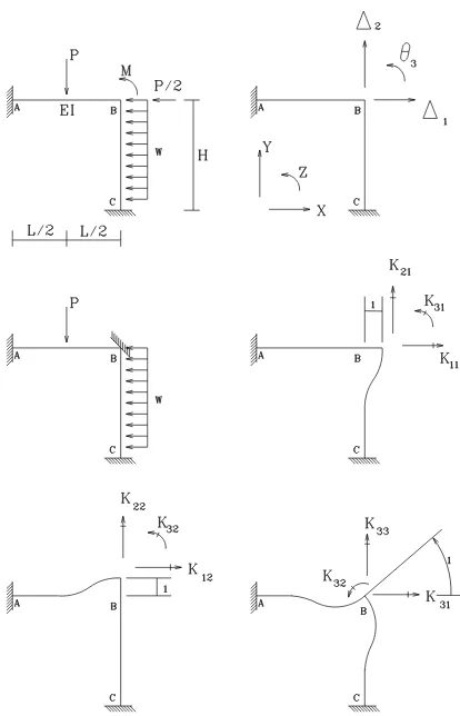
3.1

Problem with 2 Global d.o.f.

θ

1

and

θ

2

. . . 3 –3

3.2

*Frame Example (correct

K

23

) . . . 3 –6

3 .3

Grid Example . . . 3 –10

5.2

Flowchart for Assembling Global Stiffness Matrix . . . 5–5

5.3 Example of Bandwidth . . . 5–7

5.4

Numbering Schemes for Simple Structure . . . 5–7

5.5

Beam Element . . . 5–10

5.6

ID Values for Simple Beam . . . 5–20

5.7

Simple Frame Anlysed with the MATLAB Code . . . 5–20

5.8

Simple Frame Anlysed with the MATLAB Code . . . 5–22

5.9

Program Flowchart . . . 5–27

5.10 Program’s Tree Structure . . . 5–28

5.11 Flowchart for the Skyline Height Determination . . . 5–3 0

5.12 Flowchart for the Global Stiffness Matrix Assembly . . . 5–3 1

5.13 Flowchart for the Load Vector Assembly . . . 5–33

5.14 Flowchart for the Internal Forces . . . 5–3 4

5.15 Flowchart for the Reactions . . . 5–3 5

5.16 Structure Plotted with CASAP . . . 5–56

6.1

Example of [

_B

] Matrix for a Statically Determinate Truss . . . 6–3

6.2

Example of [

_B

] Matrix for a Statically Determinate Beam . . . 6–5

6.3Example of [

_B

] Matrix for a Statically Indeterminate Truss . . . 6–7

6.4

*Examples of Kinematic Instability . . . 6–13

6.5

Example 1, Congruent Transfer . . . 6–19

6.6

Example 2 . . . 6–21

7.1

Stable and Statically Determinate Element . . . 7–6

7.2

Example 1, [

k

]

_→

[

d

] . . . 7–7

8.1

Stress Components on an Infinitesimal Element . . . 8–1

8.2

Stress Traction Relations

. . . 8–2

8.3Equilibrium of Stresses, Cartesian Coordinates . . . 8–4

8.4

Fundamental Equations in Solid Mechanics . . . 8–8

Draft

LIST OFFIGURES

0–3

9.12 Variable Cross Section Fixed Beam . . . 9–3 8

9.13Uniformly Loaded Simply Supported Beam Analysed by the Rayleigh-Ritz Method9–42

9.14 Example xx: External Virtual Work . . . 9–44

9.15 Summary of Variational Methods . . . 9–50

9.16 Duality of Variational Principles . . . 9–51

10.1 Axial Finite Element . . . 10–2

10.2 Flexural Finite Element . . . 10–4

10.3 Shape Functions for Flexure of Uniform Beam Element. . . 10–6

10.4 *Constant Strain Triangle Element . . . 10–7

10.5 Constant Strain Quadrilateral Element . . . 10–10

10.6 Solid Trilinear Rectangular Element . . . 10–11

13 .1 Euler Column . . . 13 –1

13.2 Simply Supported Beam Column; Differential Segment; Effect of Axial Force P . 13–4

13.3 Solution of the Tanscendental Equation for the Buckling Load of a Fixed-Hinged

Draft

List of Tables

1.1

Example of Nodal Definition

. . . 1–5

1.2

Example of Element Definition . . . 1–5

1.3 Example of Group Number . . . 1–6

1.4

Degrees of Freedom of Different Structure Types Systems . . . 1–12

2.1

Examples of Influence Coefficients . . . 2–2

6.1

Internal Element Force Definition for the Statics Matrix . . . 6–2

6.2

Conditions for Static Determinacy, and Kinematic Instability . . . 6–13

9.1

Essential and Natural Boundary Conditions . . . 9–5

9.2

Possible Combinations of Real and Hypothetical Formulations . . . 9–20

9.3 Comparison of 2 Alternative Approximate Solutions . . . 9–49

9.4

Summary of Variational Terms Associated with One Dimensional Elements . . . 9–52

Draft

LIST OFTABLES

0–3

NOTATION

a

Vector of coefficcients in assumed displacement field

A

Area

A

Kinematics Matrix

b

Body force vector

B

Statics Matrix, relating external nodal forces to internal forces

[

B

′

]

Statics Matrix relating nodal load to internal forces

p

= [

B

′

]

P

[

B

]

Matrix relating assumed displacement fields parameters to joint displacements

C

Cosine

[

C

1

_|

C

2]

Matrices derived from the statics matrix

{

d

_}

Element flexibility matrix (lc)

{

d

c

}

[

D

]

Structure flexibility matrix (GC)

E

Elastic Modulus

[

E

]

Matrix of elastic constants (Constitutive Matrix)

{

F

_}

Unknown element forces and unknown support reactions

{

F

0

}

Nonredundant element forces (lc)

{

Fx

_}

Redundant element forces (lc)

{

F

e

}

Element forces (lc)

FEA

Fixed end actions of a restrained member

G

Shear modulus

I

Moment of inertia

[

_L

]

Matrix relating the assumed displacement field parameters

to joint displacements

[

I

]

Idendity matrix

[

ID

]

Matrix relating nodal dof to structure dof

J

St Venant’s torsional constant

[

k

]

Element stiffness matrix (lc)

[

p

]

Matrix of coefficients of a polynomial series

[

k

g

]

Geometric element stiffness matrix (lc)

[

k

r

]

Rotational stiffness matrix ( [

d

] inverse )

[

K

]

Structure stiffness matrix (GC)

[

K

g

]

Structure’s geometric stiffness matrix (GC)

L

Length

L

Linear differential operator relating displacement to strains

l

ij

Direction cosine of rotated axis i with respect to original axis j

{

LM

_}

structure dof of nodes connected to a given element

{

N

_}

Shape functions

{

p

_}

Element nodal forces = F (lc)

t

Traction vector

t

Specified tractions along Γ

t

u

Displacement vector

˜

u

Neighbour function to

u

(

x

)

u

(

x

)

Specified displacements along Γ

u

u, v, w

Translational displacements along the x, y, and z directions

U

Strain energy

U

∗

Complementary strain energy

x, y

loacal coordinate system (lc)

X, Y

Global coordinate system (GC)

W

Work

α

Coefficient of thermal expansion

[

Γ

]

Transformation matrix

{

δ

_}

Element nodal displacements (lc)

{

∆

_}

Nodal displacements in a continuous system

{

∆

_}

Structure nodal displacements (GC)

ǫ

Strain vector

ǫ

0

Initial strain vector

{

Υ

_}

Element relative displacement (lc)

{

Υ

0

}

Nonredundant element relative displacement (lc)

{

Υ

x

}

Redundant element relative displacement (lc)

θ

rotational displacement with respect to z direction (for 2D structures)

δ

Variational operator

δM

Virtual moment

δP

Virtual force

δθ

Virtual rotation

δu

Virtual displacement

δφ

Virtual curvature

δU

Virtual internal strain energy

δW

Virtual external work

δ

ǫ

Virtual strain vector

δ

σ

Virtual stress vector

Γ

Surface

Γ

t

Surface subjected to surface tractions

Γ

u

Surface associated with known displacements

σ

Stress vector

σ

0

Initial stress vector

Ω

Volume of body

Draft

Chapter 1

INTRODUCTION

1.1

Why Matrix Structural Analysis?

1

In most Civil engineering curriculum, students are required to take courses in: Statics,

Strength of Materials, Basic Structural Analysis. This last course is a fundamental one which

introduces basic structural analysis (determination of reactions, deflections, and internal forces)

of both statically determinate and indeterminate structures.

2

Also Energy methods are introduced, and most if not all examples are two dimensional. Since

the emphasis is on hand solution, very seldom are three dimensional structures analyzed. The

methods covered, for the most part lend themselves for “back of the envelope” solutions and

not necessarily for computer implementation.

3

Those students who want to pursue a specialization in structural engineering/mechanics, do

take more advanced courses such as Matrix Structural Analysis and/or Finite Element Analysis.

4

Matrix Structural Analysis, or Advanced Structural Analysis, or Introduction to Structural

Engineering Finite Element, builds on the introductory analysis course to focus on those

meth-ods which lend themselves to computer implementation. In doing so, we will place equal

emphasis on both two and three dimensional structures, and develop a thorough understanding

of computer aided analysis of structures.

5

This is essential, as in practice most, if not all, structural analysis are done by the computer

and it is imperative that as structural engineers you understand what is inside those “black

boxes”, develop enough self assurance to be capable of opening them and modify them to

perform certain specific tasks, and most importantly to understand their limitations.

7

Whereas two and three dimensional continuum are essential in civil engineering to model

structures such as dams, shells, and foundation, the majority of Civil engineering structures

are constituted by “rod” one-dimensional elements such as beams, girders, or columns. For

those elements, “displacements” and internal “forces” are somehow more complex than those

encountered in continuum finite elements.

8

Hence, contrarily to continuum finite element where displacement is mostly synonymous with

translation, in one dimensional elements, and depending on the type of structure, generalized

displacements may include translation, and/or flexural and/or torsional rotation. Similarly,

“internal forces” are not stresses, but rather axial and shear forces, and/or flexural or torsional

moments. Those concepts are far more relevant in the analysis/design of most civil engineering

structures.

9

Hence, Matrix Structural Analysis, is truly a bridge course between introductory analysis

and finite element courses. The element stiffness matrix [

k

] will first be derived using methods

introduced in basic structural analysis, and later using energy based concepts. This later

approach is the one exclusively used in the finite element method.

10

An important component of this course is computer programing. Once the theory and the

algorithms are thoroughly explained, you will be expected to program them in either Fortran

(preferably 90) or C (sorry, but no Basic) on the computer of your choice. The program

(typically about 3,500 lines) will perform the analysis of 2 and 3 dimensional truss and frame

structures, and many students have subsequently used it in their professional activities.

11

There will be one computer assignment in which you will be expected to perform

sim-ple symbolic manipulations using

Mathematica

. For those of you unfamiliar with the

Bechtel

Laboratory

, there will be a special session to introduce you to the operation of Unix on Sun

workstations.

1.2

Overview of Structural Analysis

12

To put things into perspective, it may be helpful to consider classes of Structural Analysis

which are distinguished by:

1. Excitation model

(a) Static

(b) Dynamic

2. Structure model

(a) Global geometry

Draft

1.2 Overview of Structural Analysis

1–3

•

large deformation (

ε

x

=

du_dx

+

1₂

dv dx

2

, P-∆ effects), chapter 13

(b) Structural elements element types:

•

1D framework (truss, beam, columns)

•

2D finite element (plane stress, plane strain, axisymmetric, plate or shell

ele-ments), chapter 12

•

3D finite element (solid elements)

(c) Material Properties:

•

Linear

•

Nonlinear

(d) Sectional properties:

•

Constant

•

Variable

(e) Structural connections:

•

Rigid

•

Semi-flexible (linear and non-linear)

(f) Structural supports:

•

Rigid

•

Elastic

3. Type of solution:

(a) Continuum, analytical, Partial Differential Equation

(b) Discrete, numerical, Finite ELement, Finite Difference, Boundary Element

13

Structural design must satisfy:

1. Strength (

σ < σ

f

)

2. Stiffness (“small” deformations)

3. Stability (buckling, cracking)

14

Structural analysis must satisfy

1. Statics (equilibrium)

15

Prior to analysis, a structure must be idealized for a suitable mathematical representation.

Since it is practically impossible (and most often unnecessary) to model every single detail,

assumptions must be made. Hence, structural idealization is as much an art as a science.

Some

of the questions confronting the analyst include:

1. Two dimensional versus three dimensional; Should we model a single bay of a building,

or the entire structure?

2. Frame or truss, can we neglect flexural stiffness?

3. Rigid or semi-rigid connections (most important in steel structures)

4. Rigid supports or elastic foundations (are the foundations over solid rock, or over clay

which may consolidate over time)

5. Include or not secondary members (such as diagonal braces in a three dimensional

anal-ysis).

6. Include or not axial deformation (can we neglect the axial stiffness of a beam in a

build-ing?)

7. Cross sectional properties (what is the moment of inertia of a reinforced concrete beam?)

8. Neglect or not haunches (those are usually present in zones of high negative moments)

9. Linear or nonlinear analysis (linear analysis can not predict the peak or failure load, and

will underestimate the deformations).

10. Small or large deformations (In the analysis of a high rise building subjected to wind

load, the moments should be amplified by the product of the axial load times the lateral

deformation,

P

₋

∆ effects).

11. Time dependent effects (such as creep, which is extremely important in prestressed

con-crete, or cable stayed concrete bridges).

12. Partial collapse or local yielding (would the failure of a single element trigger the failure

of the entire structure?).

13. Load static or dynamic (when should a dynamic analysis be performed?).

14. Wind load (the lateral drift of a high rise building subjected to wind load, is often the

major limitation to higher structures).

15. Thermal load (can induce large displacements, specially when a thermal gradient is

present.).

Draft

1.3 Structural Idealization

1–5

1.3.1

Structural Discretization

16

Once a structure has been idealized, it must be discretized to lend itself for a mathematical

representation which will be analyzed by a computer program. This discretization should

uniquely define each node, and member.

17

The node is characterized by its nodal id (node number), coordinates, boundary conditions,

and load (this one is often defined separately), Table 1.1. Note that in this case we have two

Node No.

Coor.

B. C.

X

Y

X

Y

Z

1

0.

0.

1

1

0

2

5.

5.

0

0

0

3

20.

5.

0

0

0

4

25.

2.5

1

1

1

Table 1.1: Example of Nodal Definition

nodal coordinates, and three degrees of freedom (to be defined later) per node. Furthermore,

a 0 and a 1 indicate unknown or known displacement. Known displacements can be zero

(restrained) or non-zero (as caused by foundation settlement).

18

The element is characterized by the nodes which it connects, and its group number, Table

1.2.

Element

From

To

Group

No.

Node

Node

Number

1

1

2

1

2

3

2

2

3

3

4

2

Table 1.2: Example of Element Definition

19

Group number will then define both element type, and elastic/geometric properties. The

last one is a pointer to a separate array, Table 1.3. In this example element 1 has element code

1 (such as beam element), while element 2 has a code 2 (such as a truss element). Material

group 1 would have different elastic/geometric properties than material group 2.

No.

Type

Group

1

1

1

2

2

1

3

1

2

Table 1.3: Example of Group Number

each element), and a sign convention become apparent.

1.3.2

Coordinate Systems

22

We should differentiate between 2 coordinate systems:

Global:

to describe the structure nodal coordinates. This system can be arbitrarily selected

provided it is a Right Hand Side (RHS) one, and we will associate with it upper case axis

labels,

X, Y, Z

, Fig. 1.1 or 1,2,3(running indeces within a computer program).

Local:

system is associated with each element and is used to describe the element internal

forces. We will associate with it lower case axis labels,

x, y, z

(or 1,2,3), Fig. 1.2.

23

The

x

-axis is assumed to be along the member, and the direction is chosen such that it points

from the 1st node to the 2nd node, Fig. 1.2.

24

Two dimensional structures will be defined in the X-Y plane.

1.3.3

Sign Convention

25

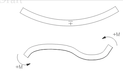
The sign convention in structural analysis is completely different than the one previously

adopted in structural analysis/design, Fig. 1.3(where we focused mostly on flexure and defined

a positive moment as one causing “tension below”. This would be awkward to program!).

26

In matrix structural analysis the sign convention adopted is consistent with the prevailing

coordinate system. Hence, we define a positive moment as one which is counter-clockwise, Fig.

1.3

27

Fig. 1.4 illustrates the sign convention associated with each type of element.

Draft

1.3 Structural Idealization

1–7

Draft

1.4 Degrees of Freedom

1–9

Figure 1.3: Sign Convention, Design and Analysis

1.4Degrees of Freedom

29

A degree of freedom (d.o.f.) is an independent generalized nodal displacement of a node.

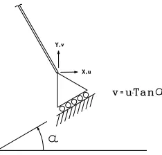
30

The displacements must be linearly independent and thus not related to each other. For

example, a roller support on an inclined plane would have three displacements (rotation

θ

, and

two translations

u

and

v

), however since the two displacements are kinematically constrained,

we only have two independent displacements, Fig. 1.5.

31

We note that we have been referring to

generalized

displacements, because we want this term

to include translations as well as rotations. Depending on the type of structure, there may

be none, one or more than one such displacement. It is unfortunate that in most introductory

courses in structural analysis, too much emphasis has been placed on two dimensional structures,

and not enough on either three dimensional ones, or two dimensional ones with torsion.

32

In most cases, there is the same number of d.o.f in local coordinates as in the global coordinate

system. One notable exception is the truss element. In local coordinate we can only have one

axial deformation, whereas in global coordinates there are two or three translations in 2D and

3D respectively for each node.

Draft

1.5 Course Organization

1–11

Figure 1.5: Independent Displacements

34

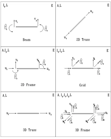
This table shows the degree of freedoms and the corresponding generalized forces.

35

We should distinguish between local and global d.o.f.’s. The numbering scheme follows the

following simple rules:

Local:

d.o.f. for a given element: Start with the first node, number the local d.o.f. in the same

order as the subscripts of the relevant local coordinate system, and repeat for the second

node.

Global:

d.o.f. for the entire structure: Starting with the 1st node, number all the unrestrained

global d.o.f.’s, and then move to the next one until all global d.o.f have been numbered,

Fig. 1.6.

Type

Node 1

Node 2

[

k

]

[

K

]

(Local)

(Global)

1 Dimensional

{

p

_}

F

y1

,

M

z2

F

y3

,

M

z4

Beam

4

_×

4

4

_×

4

{

δ

_}

v

1

,

θ

2

v

3

,

θ

4

2 Dimensional

{

p

_}

F

x1

F

x2

Truss

2

_×

2

4

_×

4

{

δ

_}

u

1

u

2

{

p

_}

F

x1

,

F

y2

,

M

z3

F

x4

,

F

y5

,

M

z6

Frame

6

_×

6

6

_×

6

{

δ

_}

u

1

,

v

2

,

θ

3

u

4

,

v

5

,

θ

6

{

p

_}

T

x1

,

F

y2

,

M

z3

T

x4

,

F

y5

,

M

z6

Grid

6

_×

6

6

_×

6

{

δ

_}

θ

1

,

v

2

,

θ

3

θ

4

,

v

5

,

θ

6

3Dimensional

{

p

_}

F

x1

,

F

x2

Truss

2

_×

2

6

_×

6

{

δ

_}

u

1

,

u

2

{

p

_}

F

x1

,

F

y2

,

F

y3

,

F

x7

,

F

y8

,

F

y9

,

T

x4

M

y5

,

M

z6

T

x10

M

y11

,

M

z12

Frame

12

_×

12

12

_×

12

{

δ

_}

u

1

,

v

2

,

w

3

,

u

7

,

v

8

,

w

9

,

θ

4

,

θ

5

θ

6

θ

10

,

θ

11

θ

12

Draft

1.5 Course Organization

1–13

Draft

Part I

Draft

Chapter 2

ELEMENT STIFFNESS MATRIX

2.1

Introduction

1

In this chapter, we shall derive the element stiffness matrix [

k

] of various one dimensional

elements. Only after this important step is well understood, we could expand the theory and

introduce the structure stiffness matrix [

K

] in its global coordinate system.

2

As will be seen later, there are two fundamentally different approaches to derive the stiffness

matrix of one dimensional element. The first one, which will be used in this chapter, is based on

classical methods of structural analysis (such as moment area or virtual force method). Thus,

in deriving the element stiffness matrix, we will be reviewing concepts earlier seen.

3

The other approach, based on energy consideration through the use of assumed shape

func-tions, will be examined in chapter 11. This second approach, exclusively used in the finite

element method, will also be extended to two and three dimensional continuum elements.

2.2

Influence Coefficients

4

In structural analysis an influence coefficient

C

_ij

can be defined as the effect on d.o.f.

i

due to

a unit action at d.o.f.

j

for an individual element or a whole structure. Examples of Influence

Coefficients are shown in Table 2.1.

Influence Line

Load

Shear

Influence Line

Load

Moment

Influence Line

Load

Deflection

Flexibility Coefficient

Load

Displacement

Stiffness Coefficient

Displacement

Load

Table 2.1: Examples of Influence Coefficients

2.3

Flexibility Matrix (Review)

6

Considering the simply supported beam shown in Fig. 2.1, and using the local coordinate

system, we have

δ

1

Using the virtual work, or more specifically, the virtual force method to analyze this problem,

(more about energy methods in Chapter 9), we have:

l

z

,

δP

and ∆ are the virtual internal force, real internal displacement, virtual

external load, and real external displacement respectively. Here, both the external virtual force

and moment are usualy taken as unity.

Virtual Force

:

Draft

2.3 Flexibility Matrix (Review)

2–3

EI

1

δM

d

11 ∆

=

0

1

₋

x

L

δM·M

dx

=

L

3

(2.4)

Similarly, we would obtain:

EId

22

=

L

0

_x

L

2

dx

=

L

3

(2.5)

EId

12

=

L

0

1

₋

x

L

_x

L

dx

=

−

L

6

=

EId

21

(2.6)

7

Those results can be summarized in a matrix form as:

[

d

] =

L

6

EI

z

2

₋

1

−

1

2

(2.7)

8

The flexibility method will be covered in more detailed, in chapter 7.

2.4Stiffness Coefficients

9

In the flexibility method, we have applied a unit force at a time and determined all the

induced displacements in the statically determinate structure.

10

In the stiffness method, we

1. Constrain all the degrees of freedom

2. Apply a unit displacement at each d.o.f. (while restraining all others to be zero)

3. Determine the reactions associated with all the d.o.f.

{

p

_}

= [

k

]

_{

δ

_}

(2.8)

11

Hence

k

_ij

will correspond to the reaction at dof

i

due to a unit deformation (translation or

rotation) at dof

j

, Fig. 2.2.

12

The actual stiffness coefficients are shown in Fig. 2.3for truss, beam, and grid elements in

terms of elastic and geometric properties.

Draft

2.4 Stiffness Coefficients

2–5

Draft

2.5 Force-Displacement Relations

2–7

Figure 2.4: Flexural Problem Formulation

2.5

Force-Displacement Relations

2.5.1

Axial Deformations

14

From strength of materials, the force/displacement relation in axial members is

σ

=

Eǫ

Aσ

P

=

AE

L

∆

1

(2.9)

Hence, for a unit displacement, the applied force should be equal to

AE_L

. From statics, the force

at the other end must be equal and opposite.

2.5.2

Flexural Deformation

15

Our objective is to seek a relation for the shear and moments at each end of a beam, in terms

of known displacements and rotations at each end.

V

1

=

V

1

(

v

1

, θ

1

, v

2

, θ

2

)

(2.10-a)

M

1

=

M

1

(

v

1

, θ

1

, v

2

, θ

2

)

(2.10-b)

V

2

=

V

2

(

v

1

, θ

1

, v

2

, θ

2

)

(2.10-c)

M

2

=

M

2

(

v

1

, θ

1

, v

2

, θ

2

)

(2.10-d)

−

EIv

′

=

M

1

x

−

1

2

V

1

x

2

₊

_C

1

(2.12)

−

EIv

=

1

2

M

1

x

2

₋

1

6

V

1

x

3

₊

_C

1

x

+

C

2

(2.13)

18

Applying the boundary conditions at

x

= 0

v

′

=

θ

1

v

=

v

1

⇒

C

1

=

−

EIθ

1

C

2

=

−

EIv

1

(2.14)

19

Applying the boundary conditions at

x

=

L

and combining with the expressions for

C

₁

and

C

2

v

′

₌

_θ

₂

v

=

v

2

⇒

−

EIθ

2

=

M

1

L

−

1₂

V

1

L

2

−

EIθ

1

−

EIv

2

=

1₂

M

1

L

2

−

₆1

V

1

L

3

−

EIθ

1

L

−

EIv

1

(2.15)

20

Since equilibrium of forces and moments must be satisfied, we have:

V

1

+

V

2

= 0

M

1

−

V

1

L

+

M

2

= 0

(2.16)

or

V

1

=

(

M

1

+

M

2

)

L

V

2

=

−

V

1

(2.17)

21

Substituting

V

₁

into the expressions for

θ

₂

and

v

₂

in Eq. 2.15 and rearranging

M

1

−

M

2

=

2EI_Lz

θ

1

−

2EI_Lz

θ

2

2

M

1

−

M

2

=

6EI_Lz

θ

1

+

6EI_L2z

v

1

−

6EI_L2z

v

2

(2.18)

22

Solving those two equations, we obtain:

M

1

=

2

EI

z

L

(2

θ

1

+

θ

2

) +

6

EI

z

L

2

(

v

1

−

v

2

)

(2.19)

M

2

=

2

EI

z

L

(

θ

1

+ 2

θ

2

) +

6

EI

z

L

2

(

v

1

−

v

2

)

(2.20)

23

Finally, we can substitute those expressions in Eq. 2.17

V

1

=

6

EI

z

L

2

(

θ

1

+

θ

2

) +

12

EI

z

L

3

(

v

1

−

v

2

)

(2.21)

V

2

=

−

6

EI

z

L

2

(

θ

1

+

θ

2

)

−

12

EI

z

Draft

2.5 Force-Displacement Relations

2–9

Figure 2.5: Torsion Rotation Relations

2.5.3

Torsional Deformations

24

From Fig. 2.2-d. Since torsional effects are seldom covered in basic structural analysis, and

students may have forgotten the derivation of the basic equations from the Strength of Material

course, we shall briefly review them.

25

Assuming a linear elastic material, and a linear strain (and thus stress) distribution along

the radius of a circular cross section subjected to torsional load, Fig. 2.5 we have:

T

=

A

ρ

c

τ

max

stress

dA

area

F orce

ρ

arm

torque

(2.23)

=

τ

max

c

A

ρ

2

dA

J

(2.24)

τ

max

=

T c

J

(2.25)

Note the analogy of this last equation with

σ

=

M c_I

z

.

26

A

ρ

2

_dA

_{is the polar moment of inertia}

_J

_{. It is also referred to as the St. Venant’s torsion}

constant. For circular cross sections

J

=

A

ρ

2

dA

=

c

0

ρ

2

(2

πρdρ

)

=

πc

4

2

=

πd

4

1 +

_db

For other sections,

J

is often tabulated.

27

Note that

J

corresponds to

I

_x

where

x

is the axis along the element.

28

Having developed a relation between torsion and shear stress, we now seek a relation between

torsion and torsional rotation. In Fig. 2.5-b, we consider the arc length BD

γ

max

dx

=

d

Φ

c

⇒

ddxΦ

=

γmax c

γ

max

=

τmax_G     

dΦ

dx

=

τmaxGc

τ

max

=

T C_J     

d

Φ

dx

=

T

GJ

(2.28)

29

Finally, we can rewrite this last equation as

T dx

=

Gjd

Φ and obtain:

T

=

GJ

L

Φ

(2.29)

Note the similarity between this equation and Equation 2.9.

2.5.4Shear Deformation

30

In general, shear deformations are quite small. However, for beams with low span to depth

ratio, those deformations can not be neglected.

31

Considering an infinitesimal element subjected to shear, Fig. 2.6 and for linear elastic

ma-terial, the shear strain (assuming small displacement, i.e. tan

γ

_≈

γ

) is given by

tan

γ

_≈

γ

=

dv

s

dx

Kinematics

=

τ

G

M aterial

(2.30)

where

dvs

dx

is the slope of the beam neutral axis from the horizontal while the vertical sections

remain undeformed,

G

is the shear modulus,

τ

the shear stress, and

v

s

the shear induced

displacement.

32

In a beam cross section, the shear stress is not constant. For example for rectangular sections,

it varies parabolically, and in I sections, the flange shear components can be neglected.

τ

=

V Q

Ib

(2.31)

Draft

2.5 Force-Displacement Relations

2–11

τ

τ

τ

τ

dvs

dx y

x

γ

γ

γ =

Figure 2.6: Deformation of an Infinitesimal Element Due to Shear

to be determined,

I

is the moment of inertia of the cross sectional area about the neutral axis,

and

b

is the width of the rectangular beam.

33

The preceding equation can be simplified as

τ

=

V

A

s

(2.32)

where

A

s

is the effective cross section for shear (which is the ratio of the cross sectional area

to the area shear factor)

34

Let us derive the expression of

A

_s

for rectangular sections. The exact expression for the

shear stress is

τ

=

V Q

Ib

(2.33)

where

Q

is the moment of the area from the external fibers to

y

with respect to the neutral

axis; For a rectangular section, this yields

τ

=

V Q

Ib

(2.34-a)

=

V

Ib

h/2

y

by

′

dy

′

=

V

2

I

h

2

4

−

y

2

(2.34-b)

=

6

V

bh

3

h

2

4

−

4

τ

=

V Q_Ib

=

k

V_A

Q

=

h/2

y

by

′

_dy

′

₌

b

2

h

2

4

−

y

2

        

k

=

₂A_Ih₄2

₋

y

2

λ bh

A

=

A

k

2

_dydz

      

λ

= 1

.

2

(2.35)

Thus, the form factor

λ

may be taken as 1.2 for rectangular beams of ordinary proportions,

and

A

s

= 1

.

2

A

For I beams,

k

can be also approximated by 1.2, provided

A

is the area of the web.

35

Combining Eq. 2.31 and 2.32 we obtain

dv

s

dx

=

V

GA

s

(2.36)

Assuming

V

to be constant, we integrate

v

s

=

V

GA

s

x

+

C

1

(2.37)

36

If the displacement

v

_s

is zero at the opposite end of the beam, then we solve for

C

₁

and

obtain

v

s

=

−

V

GA

s

(

x

₋

L

)

(2.38)

37

We define

Φ

def

=

12

EI

GA

s

L

2

(2.39)

=

24(1 +

ν

)

A

A

s

_r

L

2

(2.40)

Hence for small slenderness ratio

_Lr

compared to unity, we can neglect Φ.

38

Next, we shall consider the effect of shear deformations on both translations and rotations

Effect on Translation

Due to a unit vertical translation, the end shear force is obtained from

Eq. 2.21 and setting

v

1

= 1 and

θ

1

=

θ

2

=

v

2

= 0, or

V

=

12_LEI3z

. At

x

= 0 we have, Fig.

2.7

v

s

=

_GAV L_s

V

=

12EIz L3

Φ =

_GA12EI

sL2    



v

s

= Φ

(2.41)

Draft

2.6 Putting it All Together,

[

k

]

2–13

1

β

6EI 6EI

12EI 12EI

L2

L2

L3

L3

Figure 2.7: Effect of Flexure and Shear Deformation on Translation at One End

Effect on Rotation

Considering the beam shown in Fig. 2.8, even when a rotation

θ

1

is

applied, an internal shear force is induced, and this in turn is going to give rise to shear

deformations (translation) which must be accounted for. The shear force is obtained from

Eq. 2.21 and setting

θ

1

= 1 and

θ

2

=

v

1

=

v

2

= 0, or

V

=

6EI_L2z

. As before

v

s

=

_GAV L_s

V

=

6EIz L2

Φ =

_GA12EI

sL2    



v

s

= 0

.

5Φ

L

(2.42)

in other words, the shear deformation has moved the end of the beam (which was supposed

to have zero translation) by 0

.

5Φ

L

.

2.6

Putting it All Together,

[

k

]

39

Using basic structural analysis methods we have derived various force displacement relations

for axial, flexural, torsional and shear imposed displacements. At this point, and keeping in

mind the definition of degrees of freedom, we seek to assemble the individual element stiffness

matrices [

k

]. We shall start with the simplest one, the truss element, then consider the beam,

2D frame, grid, and finally the 3D frame element.

4EI _2EI

6EI

L _L

L2

L

0.5βLθ1

0.5βLθ1

θ1=1

Figure 2.8: Effect of Flexure and Shear Deformation on Rotation at One End

2.6.1

Truss Element

41

The truss element (whether in 2D or 3D) has only one degree of freedom associated with

each node. Hence, from Eq. 2.9, we have

[

k

t

] =

AE

L

 

u

1

u

2

p

1

1

−

1

p

2

−

1

1





(2.43)

2.6.2

Beam Element

42

There are two major beam theories:

Euler-Bernoulli

which is the classical formulation for beams.

Draft

2.6 Putting it All Together,

[

k

]

2–15

2.6.2.1

Euler-Bernoulli

43

Using Equations 2.19, 2.20, 2.21 and 2.22 we can determine the forces associated with each

unit displacement.

[

k

b

] =

    

v

1

θ

1

v

2

θ

2

V

1

Eq. 2.21(

v

1

= 1) Eq. 2.21(

θ

1

= 1)

Eq. 2.21(

v

2

= 1)

Eq. 2.21(

θ

2

= 1)

M

1

Eq. 2.19(

v

1

= 1) Eq. 2.19(

θ

1

= 1)

Eq. 2.19(

v

2

= 1)

Eq. 2.19(

θ

2

= 1)

V

2

Eq. 2.22(

v

1

= 1) Eq. 2.22(

θ

1

= 1)

Eq. 2.22(

v

2

= 1)

Eq. 2.22(

θ

2

= 1)

M

2

Eq. 2.20(

v

1

= 1) Eq. 2.20(

θ

1

= 1)

Eq. 2.20(

v

2

= 1)

Eq. 2.20(

θ

2

= 1)

    

(2.44)

44

The stiffness matrix of the beam element (neglecting shear and axial deformation) will thus

be

[

k

b

] =

        

v

1

θ

1

v

2

θ

2

V

1 12_LEI3z 6EI_L2z

−

12_LEI3z 6EI_L2z

M

1 6EI_L2z 4EI_Lz

−

6EI_L2z 2EI_Lz

V

2

−

12_LEI3z

−

6_LEI2z 12_LEI3z

−

6EI_L2z

M

2 6EI_L2z 2EI_Lz

−

6EI_L2z 4EI_Lz         

(2.45)

2.6.2.2

Timoshenko Beam

45

If shear deformations are present, we need to alter the stiffness matrix given in Eq. 2.45 in

the following manner

1. Due to translation, we must divide (or normalize) the coefficients of the first and third

columns of the stiffness matrix by 1 + Φ so that the net translation at both ends is unity.

2. Due to rotation and the effect of shear deformation

(a) The forces induced at the ends due to a unit rotation at end 1 (second column)

neglecting shear deformations are

V

1

=

−

V

2

=

6

EI

L

2

(2.46-a)

M

1

=

4

EI

L

(2.46-b)

M

2

=

2

EI

L

(2.46-c)

we should counteract this parasitic shear deformation by an equal and opposite

one. Hence, we apply an additional vertical displacement of

₋

0

.

5Φ

L

and the forces

induced at the ends (first column) are given by

V

1

=

−

V

2

=

12

EI

L

3

1

1 + Φ

kbt 11

(

₋

0

.

5Φ

L

)

vs

(2.47-a)

M

1

=

M

2

=

6

EI

L

2

1

1 + Φ

kbt 21

(

₋

0

.

5Φ

L

)

vs

(2.47-b)

Note that the denominators have already been divided by 1 + Φ in

k

bt

.

(d) Summing up all the forces, we have the forces induced as a result of a unit rotation

only when the effects of both bending and shear deformations are included.

V

1

=

−

V

2

=

6

EI

L

2

Due to Unit Rotation

+

12

EI

L

3

1

1 + Φ

kbt 11

(

₋

0

.

5Φ

L

)

vs

Due to Parasitic Shear

(2.48-a)

=

₋

6

EI

L

2

1

1 + Φ

(2.48-b)

M

1

=

4

EI

L

Due to Unit Rotation

+

6

EI

L

2

1

1 + Φ

kbt 21

(

₋

0

.

5Φ

L

)

vs

Due to Parasitic Shear

(2.48-c)

=

4 + Φ

1 + Φ

EI

L

(2.48-d)

M

2

=

2

EI

L

Due to Unit Rotation

+

6

EI

L

2

1

1 + Φ

kbt 21

(

₋

0

.

5Φ

L

)

vs

Due to Parasitic Shear

(2.48-e)

=

2

−

Φ

1 + Φ

EI

Draft

2.6 Putting it All Together,

[

k

]

2–17

46

Thus, the element stiffness matrix given in Eq. 2.45 becomes

[

k

bV

] =

2.6.3

2D Frame Element

47

The stiffness matrix of the two dimensional frame element is composed of terms from the

truss and beam elements where

k

b

and

k

t

refer to the beam and truss element stiffness matrices

respectively.

Thus, we have:

[

k

2df r

] =

49

The stiffness matrix of the grid element is very analogous to the one of the 2D frame element,

except that the axial component is replaced by the torsional one. Hence, the stiffness matrix is

[

k

g

] =

Upon substitution, the grid element stiffness matrix is given by

[

k

g

] =

50

Note that if shear deformations must be accounted for, the entries corresponding to shear

and flexure must be modified in accordance with Eq. 2.49

2.6.5

3D Frame Element

Draft

2.7 Remarks on Element Stiffness Matrices

2–19

51

Note that if shear deformations must be accounted for, the entries corresponding to shear

and flexure must be modified in accordance with Eq. 2.49

2.7

Remarks on Element Stiffness Matrices

Singularity:

All the derived stiffness matrices are singular, that is there is at least one row and

one column which is a linear combination of others. For example in the beam element,

row 4 =

₋

row 1; and L times row 2 is equal to the sum of row 3and 6. This singularity

(not present in the flexibility matrix) is caused by the linear relations introduced by the

equilibrium equations which are embedded in the formulation.

Symmetry:

All matrices are symmetric due to Maxwell-Betti’s reciprocal theorem, and the

stiffness flexibility relation.

Draft

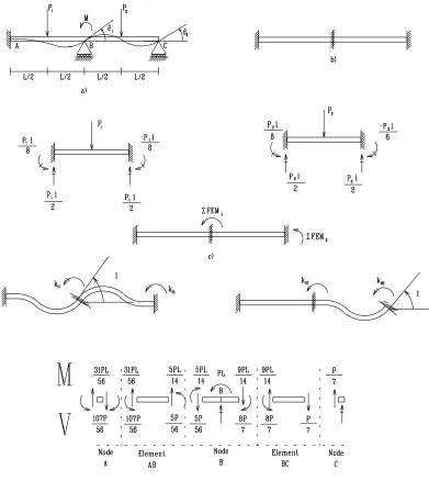
Chapter 3

STIFFNESS METHOD; Part I:

ORTHOGONAL STRUCTURES

3.1

Introduction

1

In the previous chapter we have first derived displacement force relations for different types

of rod elements, and then used those relations to define element stiffness matrices in local

coordinates.

2

In this chapter, we seek to perform similar operations, but for an orthogonal structure in

global coordinates.

3

In the previous chapter our starting point was basic displacement-force relations resulting in

element stiffness matrices [

k

].

4

In this chapter, our starting point are those same element stiffness matrices [

k

], and our

objective is to determine the structure stiffness matrix [

K

], which when inverted, would yield

the nodal displacements.

5

The element stiffness matrices were derived for fully restrained elements.

6

This chapter will be restricted to orthogonal structures, and generalization will be discussed

later.

The stiffness matrices will be restricted to the unrestrained degrees of freedom.

8

As a “vehicle” for the introduction to the stiffness method let us consider the problem in Fig

3.1-a, and recognize that there are only two unknown displacements, or more precisely, two

global d.o.f:

θ

1

and

θ

2

.

9

If we were to analyse this problem by the force (or flexibility) method, then

1. We make the structure statically determinate by removing

arbitrarily

two reactions (as

long as the structure remains stable), and the beam is now statically determinate.

2. Assuming that we remove the two roller supports, then we determine the corresponding

deflections due to the actual laod (∆

B

and ∆

C

).

3. Apply a unit load at point

B

, and then

C

, and compute the deflections

f

ij

at note

i

due

to a unit force at node

j

.

4. Write the compatibility of displacement equation

f

BB

f

BC

f

CB

f

CC

R

B

R

C

−

∆

1

∆

2

=

0

0

(3.1)

5. Invert the matrix, and solve for the reactions

10

We will analyze this simple problem by the stiffness method.

1. The first step consists in making it kinematically determinate (as opposed to statically

determinate in the flexibility method). Kinematically determinate in this case simply

means restraining all the d.o.f. and thus prevent joint rotation, Fig 3.1-b.

2. We then determine the fixed end actions caused by the element load, and sum them for

each d.o.f., Fig 3.1-c: ΣFEM

1

and ΣFEM

2

.

3. In the third step, we will apply a unit displacement (rotation in this case) at each degree

of freedom at a time, and in each case we shall determine the reaction forces,

K

11

,

K

21

,

and

K

12

,

K

22

respectively. Note that we use [

K

], rather than

k

since those are forces

in the global coordinate system, Fig 3.1-d. Again note that we are focusing only on the

reaction forces corresponding to a global degree of freedom. Hence, we are not attempting

to determine the reaction at node A.

4. Finally, we write the equation of equilibrium at each node:

M

1

M

2

=

ΣFEM

1

ΣFEM

2

+

K

11

K

12

K

21

K

22

θ

1

θ

2

Draft

3.2 The Stiffness Method

3–3