Scimago Journal & Country Rank
Home Journal Rankings Country Rankings Viz Tools Help About Us
World Development
Country United Kingdom
133
H Index
Subject Area and
Category Economics, Econometrics and FinanceEconomics and Econometrics
Social Sciences Development
Geography, Planning and Development Sociology and Political Science
Publisher Elsevier Ltd.
Publication type Journals
ISSN 0305750X
Coverage 1973-ongoing
Scope World Development is a multi-disciplinary monthly journal of development studies. It seeks to explore ways of improving standards of living, and the human condition generally, by
examining potential solutions to problems such as: poverty, unemployment, malnutrition, disease, lack of shelter, environmental degradation, inadequate scienti c and technological resources, trade and payments imbalances, international debt, gender and ethnic
discrimination, militarism and civil con ict, and lack of popular participation in economic and political life. Contributions offer constructive ideas and analysis, and highlight the lessons to be learned from the experiences of different nations, societies, and economies. (source)
Enter Journal Title, ISSN or Publisher Name
Quartiles
The set of journals have been ranked according to their SJR and divided into four equal groups, four quartiles. Q1 (green) comprises the quarter of the journals with the highest values, Q2 (yellow) the second highest values, Q3 (orange) the third highest values and Q4 (red) the lowest values.
Category Year Quartile
Development 1997 Q1
Development 1998 Q1
Development 1999 Q1
Development 2000 Q1
SJR
The SJR is a size-independent prestige indicator that ranks journals by their 'average prestige per article'. It is based on the idea that 'all citations are not created
Citations per document
This indicator counts the number of citations received by documents from a journal and divides them by the total number of documents published in that journal.
1997 1999 2001 2003 2005 2007 2009 2011 2013 2015
Development
Economics and Econometrics
Geography, Planning and Development
equal'. SJR is a measure of scienti c in uence of journals that accounts for both the number of citations received by a journal and the importance or prestige of the journals where such citations come from It measures the scienti c in uence of the average article in a journal, it expresses how central to the global
The chart shows the evolution of the average number of times documents published in a journal in the past two, three and four years have been cited in the current year. The two years line is equivalent to journal impact factor
™ (Thomson Reuters) metric.
Cites per document Year Value
Cites / Doc. (4 years) 1999 1.354 Cites / Doc. (4 years) 2000 1.335 Cites / Doc. (4 years) 2001 1.742 Cites / Doc. (4 years) 2002 1.719 Cites / Doc. (4 years) 2003 2.253 Cites / Doc. (4 years) 2004 2.503 Cites / Doc. (4 years) 2005 3.078 Cites / Doc. (4 years) 2006 2.867 Cites / Doc. (4 years) 2007 3.231 Cites / Doc. (4 years) 2008 3.391
Total Cites Self-Cites
Evolution of the total number of citations and journal's self-citations received by a journal's published
documents during the three previous years.
Journal Self-citation is de ned as the number of citation from a journal citing article to articles published by the same journal.
Cites Year Value
Self Cites 1999 69
External Cites per Doc Cites per Doc
Evolution of the number of total citation per document and external citation per document (i.e. journal self-citations removed) received by a journal's published documents during the three previous years. External citations are calculated by subtracting the number of self-citations from the total number of citations received by the journal’s documents.
Cites Year Value
% International Collaboration
International Collaboration accounts for the articles that have been produced by researchers from several
countries. The chart shows the ratio of a journal's documents signed by researchers from more than one country; that is including more than one country address.
Year International Collaboration
1999 15.08
Citable documents Non-citable documents
Not every article in a journal is considered primary research and therefore "citable", this chart shows the ratio of a journal's articles including substantial research (research articles, conference papers and reviews) in three year windows vs. those documents other than research articles, reviews and conference papers.
Documents Year Value
Cited documents Uncited documents
Ratio of a journal's items, grouped in three years windows, that have been cited at least once vs. those not cited during the following year.
Documents Year Value
Uncited documents 1999 200 Uncited documents 2000 196 Uncited documents 2001 140 Uncited documents 2002 140
Show this widget in your own website
Just copy the code below and paste within your html code:
<a href="http://www.scimagojr.com/journalsearch.php?q=30060&tip=sid&exact=no" title="SCImago Journal & Country Rank"><img border="0" src="http://www.scimagojr.com/journal_img.php?id=30060" alt="SCImago Journal & Country Rank" /></a> 1.4
2.1 2.8
0.6 1.2 1.8 2.4 3 3.6 4.2
1999 2001 2003 2005 2007 2009 2011 2013 2015 0
2k 4k
1999 2001 2003 2005 2007 2009 2011 2013 2015 0
2 4
1999 2002 2005 2008 2011 2014
0 20 40 60
1999 2002 2005 2008 2011 2014
0 400 800
1999 2002 2005 2008 2011 2014
Developed by:
Powered by:
Follow us on
Scimago Lab
, Copyright 2007-2017. Data Source:
Scopus®
Does Foreign Direct Investment Lead to Productivity Spillovers?
Firm Level Evidence from Indonesia
SUYANTO, RUHUL A. SALIM and HARRY BLOCH
*Curtin University of Technology, Perth, WA, Australia
Summary.—This paper examines whether spillovers from foreign direct investment (FDI) make any contribution to productivity
growth in the Indonesian chemical and pharmaceutical firms using plant-level panel data. The spillover effects from FDI are analyzed using a stochastic frontier approach and productivity growth is decomposed using a generalizedMalmquistoutput-oriented index. The results show positive productivity spillovers from FDI; higher competition is associated with larger spillovers; and domestic firms with R&D gain more spillover benefits compared to those without R&D. FDI spillovers are found to be positive and significant for techno-logical progress and positive, but not significant, for technical and scale efficiency change.
Crown CopyrightÓ2009 Published by Elsevier Ltd. All rights reserved.
Key words— FDI spillovers, frontier production function,Malmquistindex, total factor productivity growth
1. INTRODUCTION
Foreign direct investment (FDI) is believed to provide reci-pient countries with knowledge1 transfer as well as capital.
The argument is that multinational corporations (MNCs) establish subsidiaries in overseas and transfer knowledge to their subsidiaries. The transferred knowledge has a certain public good quality and may spread through non-market mechanisms over the entire economy leading to productivity gains (hereafter productivity spillovers) in domestic firms (Blomstrom, 1989).
Expectation of productivity spillovers from knowledge transfers has been a major impetus to policy makers in many countries to provide FDI-friendly regime.2
In developing countries, policies in favor of FDI have been introduced since the early 1980s. Since then, net inflows of FDI have in-creased dramatically and FDI has been the most significant part of private capital inflows to developing countries. From 1985 to 2006, for example, the net FDI inflows to developing countries have increased from US$ 14 billion to US$ 379 bil-lion, rising more than 25-folds (UNCTAD, 2007). In recent years, FDI inflows have accounted for more than half of the total private capital inflows in developing countries (Ng, 2006).
Now an important question is whether these huge FDI in-flows indeed bring about productivity spillovers for recipient countries, particularly for developing economies. The evidence is fairly mixed so far. Some empirical studies confirm positive productivity spillovers from FDI (e.g., Caves, 1974; Chakr-aborty & Nunnenkamp, 2008; Gorg & Strobl, 2005; Javorcik, 2004; Schiff & Wang, 2008), but others find negative or no spillovers (e.g., Aitken & Harrison, 1999; Barry, Gorg, & Strobl, 2005; Djankov & Hoekman, 2000; Haddad & Harri-son, 1993). The mixed evidence intuitively implies that there is no universal relationship between FDI and domestic firms’ productivity. Some studies, however, argue that the mixed findings may be attributed to domestic firms’ characteristics or host countries’ ability to absorb productivity spillovers (Gorg & Greenaway, 2004; Smeets, 2008). Nevertheless, differ-ences in findings depend significantly on research design, methodological approach, types of data used, estimation strat-egy, and even on the construction of the spillover variable.
The present paper extends the current empirical literature to determine whether the FDI leads to productivity gains in the Indonesian chemical and pharmaceutical industries during 1988–2000. These two industries have been chosen as they continuously attracted the highest inflow of annual FDI since 1975 (Table 2). They belong to the group of the most produc-tive sectors in the Indonesian manufacturing industries in terms of value added per worker (around 1.5 times of the man-ufacturing average),3while registering a consistent growth of an annual average of 17.71% during 1988–2000).4 An
over-whelming presence of MNCs in this sector provides a good basis to examine the role of firm-specific characteristics in determining the productivity spillovers.
We estimate FDI productivity spillovers using the Stochas-tic Frontier Approach (SFA). With this method we also address the importance of competition and firms’ absorptive capacity for gaining productivity spillovers. Furthermore, we identify the sources of productivity growth in the presence of FDI in these two major industries of the Indonesian economy. A generalizedMalmquist indexis used to decompose total fac-tor productivity (TFP) growth into technical efficiency change (TEC), technological progress (TP), and scale efficiency change (SEC). We then test the impact of FDI spillover effects on each of these components of productivity growth. The authors know of no other study that addresses the issue of decomposing the productivity effects of FDI using a general-izedMalmquist index.5
The rest of this paper proceeds as follows: Section 2 pro-vides an overview of the Indonesian manufacturing sector and the inflow of FDI, which is followed by a critical review of the theoretical and empirical studies on productivity spill-overs in Section 3. Section 4 discusses estimation techniques followed by data sources and variable construction. Section 6 presents the results for model selection and estimation,
* We would like to thank M.M. Kabir from the School of Economics & Finance, Curtin University of Technology and four anonymous referees for useful comments on the previous version of this article without imp-licating them for any errors that may remain. Final revision accepted: May 27, 2009.
World DevelopmentVol. 37, No. 12, pp. 1861–1876, 2009 Crown CopyrightÓ2009 Published by Elsevier Ltd. All rights reserved 0305-750X/$ - see front matter www.elsevier.com/locate/worlddev
doi:10.1016/j.worlddev.2009.05.009
followed by an analysis of empirical results. The summary of findings and policy implications is given in the final section.
2. AN OVERVIEW OF THE INDONESIAN MANUFACTURING AND FDI FLOWS
Indonesian manufacturing has been demonstrating specta-cular growth and unprecedented transformation since the sec-ond half of 1970s. This transformation is evident not only in rapid output and in employment growth, but also in the tran-sition to modern capital and skill-intensive industries, strong productivity and wage growth, and broadening the industrial base outside the capital city, along with a probable reduction in concentration levels (Hill, 1996). Decisive liberalization re-forms have been introduced since the mid 1980s. These in-cluded reduction in tariff and non-tariff barriers,6 privatization of public enterprises, relaxation of foreign invest-ment rules, and lessening other restrictions. The reform pack-age also included fiscal reform, financial liberalization, and the maintenance of a realistic and flexible exchange rate, together with trade liberalization, reduction in government intervention and improved management of public enterprises. The trial development policies were focused on the priority indus-tries and the creation of industrial zones. The reforms of the 1980s were designed to improve the productivity performance of manufacturing industries by encouraging competition from within the economy as well as from outside.
The change of policy direction from interventionist to liber-alization encourages the expansion of export-oriented sub-sec-tors, such as chemicals and pharmaceuticals (ISIC 35), and woods and wood products (ISIC 33). As a result, since 1987 Indonesia has experienced a surge in manufactured exports, for example, during the period 1989–93 manufactured exports grew at an average annual rate of 27%, while manufacturing value added (MVA) grew at an average annual rate of 22% (UNIDO, 2000). Export-oriented manufacturing firms wit-nessed a higher growth than non-export firms, and at the same time, manufacturing firms experienced a substantial produc-tivity growth.
Studies reveal that manufacturing sector experienced higher TFP (total factor productivity) growth at around 6% per an-num in the post liberalization period (Ikhsan, 2007; Vial, 2006) compared to a negative growth of4.9% during 1981– 83 (Aswicahyono, 1988). One of the important factors contrib-uting to these positive outcomes in the manufacturing sector during the post-liberalization period was a massive inflow of FDI.7The huge increase in FDI inflows, from a meager US$ 0.2 billion in 1983 to US$ 5.9 billion in 2006,8facilitated the
high growth of manufacturing industries in terms of output, employment, and value added. Moreover, the growing FDI in-flows helped create backward and forward linkages in the econ-omy. Although there was a decrease in manufacturing growth during the East Asian crisis in 1997, this sector revived quickly and demonstrated further growth since 2000.
The manufacturing sector received a large proportion of to-tal FDI inflows in the Indonesian economy. The share of ap-proved FDI to this sector accounts for more than 50% of total approved FDI over the last three decades (Table 1). Although the total approved FDI decreased steadily after the economic crisis, the share of manufacturing FDI remains the largest part of the total FDI. Furthermore, within the manufacturing sec-tor over the years (Table 2), the highest share of manufactur-ing FDI flowed to chemicals and pharmaceuticals (44.56%), followed by metal products (13.13%) and papers and paper products (11.96%). Food products have received an increasing
share of manufacturing FDI, particularly after the deregula-tion in 1984. However, the average percentage of FDI to this sector remains relatively small of the total approved manufac-turing FDI.
Based on the high level of FDI, the present study focuses on chemical and pharmaceutical firms in examining the produc-tivity spillovers of FDI. Another reason to focus on this sector rather than on pooling data for the whole Indonesian manu-facturing is to reduce heterogeneity in data, as suggested by Bartelsman and Doms (2000). Firms in the chemical and phar-maceutical sectors have different characteristics, in terms of size and technology, compared to, for example, firms in food processing sector. Pooling firms from both industries together may give rise to persistent heterogeneity in data.
The chemical and pharmaceutical sectors (ISIC 35) represent about 18% of Indonesian manufacturing output and around 12% of the manufacturing employment in 2005. This sector employs some 540 thousand people with wages of around IDR 8,445 billions per year. Its contribution to the manufac-turing value added (MVA) was the third highest of all indus-tries after the food industry and textiles. During 1975–2005, this sector expanded rapidly, increasing in value added by more than 35 times.9 It is a diverse industry ranging from large-scale petrochemical complexes to medium-sized estab-lishments that simply mix chemicals to produce paint, pesti-cide, and traditional medicines. In the Annual Survey of Manufacturing Industries, the BPS divides this sector into six sub-sectors: industrial chemicals (ISIC 351), pharmaceutical and other chemicals (352), oil and gas refining (353 and 354), rubber and products (355), and plastic products (356). Among these sub-sectors, the oil and gas refining sub-sectors have only been surveyed since 1990 and cover only a few establishments. The other four sub-sectors have been surveyed since 1975.
In this study, the focus is on the sub-sectors industrial chem-icals (ISIC 351) and pharmaceutchem-icals and other chemchem-icals (ISIC 352), as these two sub-sectors represent more than 70% of the sector value added. The trend and key indicators of the two sub-sectors (hereafter, chemical firms and pharma-ceutical firms refer to firms in these two sub-sectors, respec-tively) during the studied periods are presented in Table 3. From the table, one might note that the combined sub-sectors expanded rapidly during 1988–98, which can be observed from an increase in output and value added by more than 10 times. Labor productivity, which is measured by value added per la-bor (VA/L), also increased considerably by almost eight times during the years.
Interestingly, the number of foreign firms, as a percentage of total firms across the two sub-sectors combined, increased quite significantly from 12.92% in 1988 to 18.65% in 1998. A similar pattern is also observed for foreign share (as a percent-age of value added), as it rose drastically from 27% in 1988 to 61.23% in 1998, suggesting an important contribution of for-eign firms to the value added in this sector. The exported out-puts of the combined sub-sectors were less than 7% during 1988–98. In contrast, there was heavy reliance on imported materials, with 55.18% and 44.75% of total material was im-ported in 1988 and 1998, respectively.
3. RELATED LITERATURE AND HYPOTHESIS DEVELOPMENT
(a)MNCs, superior knowledge, and productivity spillovers
When MNCs establish subsidiaries overseas, they come across disadvantages in the form of access to resources
and domestic demand, when compared to their local coun-terparts. Domestic firms have more experience in serving domestic markets and possess more information regarding the type of products, consumer preferences, and distribu-tional networks relative to MNCs. In order to compete with the domestic firms, MNCs need to possess superior knowl-edge (Caves, 1971). The superior knowledge, which is often known as special intangible assets in the industrial organiza-tional theory of FDI, takes the form of process and prod-uct, managerial and organizational, and scale efficiency knowledge (Kokko & Kravtsova, 2008). With this superior knowledge, MNCs are often assumed to have higher perfor-mance levels than domestic firms, in particular being more
efficient and productive. To test whether this is the case in the Indonesian chemical and pharmaceutical sectors, this study hypothesizes that
H1a. Foreign-owned firms are more efficient (or productive) than domestic firms.
If MNCs indeed possess superior knowledge relative to domestic firms, there is a possibility that MNCs may generate positive productivity spillovers (Blomstrom & Kokko, 1998). When MNCs transfer knowledge to their subsidiaries, the transferred knowledge may spill, through non-market mechanisms, over the entire economy that may then lead to Table 3. Trend and key indicators of the chemical and pharmaceutical sectors
Key indicators Chemicals and pharmaceuticals (ISIC 351 and 352)
Industrial chemicals (ISIC 351)
Pharmaceuticals and other chemicals (ISIC 352)
1988 1993 1998 1988 1993 1998 1988 1993 1998 Output (billion rupiah) 4,133 11,071 42,948 2,142 5,637 27,793 1,991 5,434 15,155 Value-added (billion rupiah) 1,451 4,376 16,712 784 2,401 10,983 667 1,975 5,729 Labor (person) 114,565 160,673 192,618 39,495 60,241 81,914 75,070 100,432 110,704 VA/L (thousand rupiah) 12,668 27,236 86,760 19,850 39,853 134,074 8,889 19,669 51,751 No of establishments 743 892 1,035 218 325 431 525 567 604 Foreign firm (% of total establishments) 12.92 14.01 18.65 11.93 16.92 22.97 13.33 13.35 15.56 Domestic firm (% of total establishments) 81.16 81.28 77.10 75.23 76.00 71.69 83.81 83.30 80.96 SOEs (% of total establishments) 5.92 4.71 4.25 12.84 7.08 5.34 2.86 3.35 3.48 Foreign share (% of VA) 27.00 42.85 61.23 17.12 39.97 67.90 38.61 46.35 48.42 Export (% of output) 5.09a 6.56 1.42 8.09a 10.88 4.62 3.46a 4.08 1.29
Imported-material (% of total material) 55.18 44.48 44.75 57.01 46.02 43.05 52.97 42.83 48.15 Source: Authors’ calculation from the Annual Survey of Large and Medium Manufacturing Industries.
Foreign firms are defined as firms with any foreign ownership, domestic firms are firms those 100% owned by domestic private individual or companies, and state-owned enterprises (SOEs) are firms owned by the central or district government.
a
The figure was calculated based on the data in 1990 because it was the first year the information on export was published.
Table 2. The distribution of approved manufacturing FDI (as % of total approved manufacturing FDI) in two-digit ISIC industries for the period 1975–2006
Year Food (31) Textile and leather (32)
Wood and wood product (33)
Paper and paper product (34)
Chemical and pharmaceutical (35)
Non metal mineral (36)
Basic metal (37)
Metal products (38)
Others (39)
1975–79 4.96 8.81 0.77 2.87 15.84 9.97 47.99 8.59 0.19 1980–84 2.63 6.21 2.41 12.21 18.12 5.67 24.60 28.13 0.01 1985–89 5.40 9.14 2.83 18.69 48.25 4.61 2.74 7.92 0.42 1990–94 5.29 11.54 1.50 15.79 35.13 5.35 7.35 17.01 1.05 1995–99 5.10 2.50 0.88 14.36 58.62 3.36 3.74 11.12 0.33 2000–04 7.62 4.27 1.34 7.37 54.83 2.96 6.29 6.12 9.21 2005 10.66 2.31 1.70 3.78 47.76 6.11 0.00 11.53 16.16 2006 12.47 1.88 1.66 14.09 18.40 9.45 0.00 35.13 6.91 1975–2006 6.31 5.99 1.40 11.96 44.56 4.71 8.11 13.13 3.83 Source: Calculated from Indonesian Financial Statistics, Central Bank of Indonesia, various years.
Table 1. Share of approved manufacturing FDI 1975–2006
Year Total approved FDI (million USD) Approved manufacturing FDI (million USD) Share of manufacturing FDI to total FDI (percentages)
1975–79 5,322.10 3,666.40 68.89
1980–84 7,765.70 6,346.10 81.72
1985–89 12,300.20 10,150.10 82.52
1990–94 57,996.50 37,507.10 64.67
1995–99 126,919.20 81,092.60 63.89
2000–04 57,495.20 31,735.20 55.20
2005–06 29,203.20 14,336.10 49.09
1975–2006 297,002.10 184,833.60 62.23
Sources: Calculated from Indonesian Financial Statistics, Central Bank of Indonesia, various years.
productivity growth in domestic firms. However, MNCs would prevent their knowledge seeping to domestic firms by raising the cost of spillovers, such as patenting their products and ideas.
A large number of empirical studies examine the productiv-ity spillovers hypothesis of FDI in the literature. The pioneer-ing empirical research in this area was conducted by Caves (1974)on Australia, followed by Globerman (1979)on Can-ada, and Blomstrom and Persson (1983) on Mexico. The empirical literature then developed in many directions in a number of country-specific and cross-country investigations. However, the findings of these studies are diverse and incon-clusive.10The relationship between FDI spillovers and firms’ productivity gains still remains to be an empirical issue. Being the top recipients of FDI, the higherper capitaproductivity in Indonesian chemical and pharmaceutical industries than the manufacturing average therefore suggests a test for the follow-ing hypothesis:
H1b. There is a positive productivity spillover from FDI in the Indonesian chemical and pharmaceutical sectors.
(b)Productivity spillovers and competition
Most of the previous studies on FDI spillovers treat the spe-cific mechanisms of productivity spillovers as occurring in a ‘‘black box” (Gorg & Strobl, 2005). These studies often as-sume that productivity spillovers from FDI occur automati-cally as a consequence of foreign firms’ presence in domestic markets. The channels of productivity spillovers are not explicitly taken into account in such studies.
However, some studies try to consider explicitly the chan-nels of productivity spillovers from FDI. There are three fun-damental mechanisms for productivity spillovers to take place. First, the entry of MNCs may lead to greater competition in domestic markets, which then forces domestic firms to utilize their resources and technology in more efficient ways, leading to productivity gains (Wang & Blomstrom, 1992). Second, knowledge may spill over to domestic firmsvialabor turnover, that is, when workers trained by MNCs move to domestic firms and bring with them the knowledge and other crucial intangible assets (Fosfuri, Motta, & Ronde, 2001). Third, for-eign firms in domestic markets may create demonstration ef-fects to domestic firms through direct imitation and reverse engineering (Das, 1987), or new innovation through R&D (Cheung & Lin, 2004).
Of these three channels of productivity spillovers, the first channel is of particular interest in this study. Competition may result in either positive or negative productivity spillovers for domestic firms.Aitken and Harrison (1999)argue that, in the short-run, the presence of foreign firms in an imperfect competition domestic market may raise the average cost of production of domestic firms through the ‘‘market stealing”
phenomenon. Foreign firms with a lower marginal cost have an incentive to increase production relative to their domestic competitors. The productivity of domestic firms will fall as they have to spread fixed costs over a smaller amount of out-put. However, in the long-run, when all costs can be treated as variable costs, there is a possibility for domestic firms to re-duce their costs by allocating their resources more efficiently and imitating foreign firms’ knowledge (Wang & Blomstrom, 1992). If the efficiency effect from foreign presence is larger than the competition effect, there can be positive productivity spillovers. Following these arguments, this study tests the fol-lowing hypothesis:
H2. Higher competition is associated with larger spillovers from foreign presence in the industry, that is, positive productivity spillover through competition.
(c)Productivity spillovers and absorptive capacity
The mixed evidence of productivity spillovers leads to the celebrated argument that firm-specific characteristics (or absorptive capacity) may influence the ability of domestic firms in gaining productivity spillovers from FDI (Findlay, 1978; Glass & Saggi, 1998; Wang & Blomstrom, 1992). The most commonly used measure of absorptive capacity is the extent of research and development (R&D) expenditure. In a study of the Indian manufacturing firms, Kathuria (2000) shows that local firms that invest in learning, or R&D activ-ities receive high productivity spillovers, whereas the non-R&D local firms do not gain much from the presence of for-eign firms. This result indicates that the productivity spill-overs are not automatic consequences of the presence of foreign firms; rather they depend on the efforts of local firms’ investment in R&D activities. Kinoshita (2001)finds similar evidence in a study on Czech manufacturing firms during 1995–98. By focusing on electrical machinery and radio & TV sectors, she finds that R&D is a necessary condition for technology spillovers from FDI. In a more recent study on twelve OECD countries,Griffith, Redding, and van Ree-nen (2004)also confirm that R&D plays an important role in knowledge transfer, besides its role as a medium of innova-tion. To capture a firm-specific characteristic of Indonesian chemical and pharmaceutical firms in determining the pro-ductivity spillovers from FDI, this study also tests the follow-ing hypothesis:
H3. Domestic firms with R&D expenditure gain more pro-ductivity spillovers from FDI than those without R&D expenditure.
(d)Sources of productivity advantage from FDI
Technical and scale efficiencies are hardly studied in the lit-erature in relation to productivity gains from FDI. While the theoretical literature provides little guidance to these two sources of productivity growth, the empirical studies also tend to ignore the decomposition issue (Girma & Gorg, 2007). The empirical studies usually assume that productivity advantage from FDI is exclusively contributed by technology transfers as is consistent with the use of conventional approach of pro-duction function.11
The stochastic productivity frontier literature, such as Orea (2002), offer a parametric decomposition of productiv-ity growth into three components: technical efficiency change (TEC), technological progress (TP), and scale effi-ciency change (SEC). By decomposing productivity growth using this analysis, it is possible to examine the productivity advantage from FDI to technical and scale efficiencies as well as technological progress. In a recent survey, Smeets (2008) argues that the productivity spillovers from FDI should be defined broadly, as it arises from new knowledge rather not only from new technology. Further, he defines knowledge as including technology; managerial, and produc-tion skills, which may contribute to technical efficiency and ability to exploit scale efficiency. Therefore, the final hypoth-esis to test sources of productivity gains from FDI can be stated as follows:
H4. There are positive FDI spillovers to each component of productivity growth (TEC, TP, and SEC).
4. MODEL SPECIFICATION AND ESTIMATION TECHNIQUES
(a)Productivity spillovers from FDI: a stochastic frontier approach
When measuring efficiencies and productivity at the firm le-vel, researchers face the choice of alternative approaches, such as conventional production (cost) functions, data envelopment analysis (DEA), and stochastic frontier production (cost) function. Each of these approaches has its merits and demer-its. The debate over which approach is appropriate continues (Coelli, Rao, O’Donnell, & Battese, 2005).
We apply the stochastic frontier production function to test the spillover hypothesis from FDI. Following Battese and Coelli (1995)the stochastic frontier approach (SFA) is used to estimate a production function and an inefficiency function simultaneously.12The Battese–Coelli model can be expressed
as follows:13
yit¼fðxit;t;bÞ expðmituitÞ; ð1Þ
where yit implies the production of the ith firm (i= 1, 2,. . .,N) in thetth time period (t= 1, 2,. . .,T),xit denotes a ð1kÞ vector of explanatory variables, and b represents the (k1) vector of parameters to be estimated. The error term consists of two components:vit anduit, which are inde-pendent of each other. In addition, the vit denotes the time-specific and stochastic part, withiidNð0;r2
vÞ, and theuit repre-sents technical inefficiency, which is normal distribution, but truncated at zero with meanzitdand variancer2u.
The technical inefficiency effects,uit, are assumed as a func-tion of að1jÞvector of observable non-stochastic explana-tory variables,zit, and aðj1Þvector of unknown parameters to be estimated, d. In a linear equation, the technical ineffi-ciency effects can be specified as follows:
uit¼zitdþwit; ð2Þ
wherewitis an unobservable random variable, which is defined by the truncation of the normal distribution with zero mean and variance,r2
u, such that the point of truncation iszitd. Eqn.(1)shows the stochastic production function in terms of the original production value, and Eqn.(2)represents the technical inefficiency effects.The parameters of both equations can be estimated simultaneously by the maximum-likelihood method. The likelihood function is expressed in terms of var-iance parameters r2
zero, then the model reduces to a traditional mean response function in whichzitcan be directly included into the produc-tion funcproduc-tion.
Based on the theoretical model in Eqns.(1) and (2), we start with a flexible functional form, namely, atranslogproduction function. By adopting a flexible functional form, the risk of er-rors in the model specification can be reduced. Moreover, the
translogform is useful for decomposing the total factor pro-ductivity growth. The functional form of thetranslog produc-tion funcproduc-tion is as follows:
lnyit ¼b0þ
whereyimplies output,xrepresents variables that explain out-put (labor and capital, soN= 2),tis time,iis firm. Anduitis
wherezis the set of explanatory variables that explain techni-cal inefficiency.
Hypotheses H1a, H1b, H2, and H3 are tested by estimating three alternative technical inefficiency functions to avoid the possibility of multicollinearity. A test of H1 includes only a spillover variable; a test of H2 involves an interacting variable of spillover and competition; and a test of H3 involves an interacting variable of spillover and R&D. The interacting variables in H2 and H3 are likely to have a high correlation with each other. A simple possible way to deal with this issue in a stochastic frontier model is to estimate the hypotheses sep-arately.
To test H1, the subscriptjin Eqn.(4)represents the dummy variable of foreign ownership (to test H1a) and FDI spillovers (to test H1b). These hypotheses are tested by controlling the age of the firm.zjin Eqn.(4)includes an interacting variable of competition and spillovers when testing H2, while it repre-sents an interacting variable of R&D and spillovers when test-ing H3. Details of definition and construction of each variable used in Eqns.(3) and (4)are presented inTable A1.
Given the specifications in Eqns. (3) and (4), the technical efficiency of production for the ith firm at thetth year is de-fined as the ratio of the actual output of firmi, lnyit, to its
po-(b)Decomposing productivity growth: a generalizedMalmquist
index
Orea (2002)shows that if firmi’s technology in timetcan be represented by a translog output-oriented distance function
DO(yit,xit, t) whereyit, xit, and tare defined as above, then the logarithm of a generalized output-orientedMalmquist pro-ductivity growth index, GtOi;tþ1, can be decomposed into TEC,
TP, and SEC between time periodstandt+ 1:
where eit¼
PN
n¼1eitn is the scale elasticity such that
eitn¼@
lnDOðyit;xit;tÞ @lnxitn .
If the output is only one, then atranslogoutput-oriented dis-tance function can be defined as
lnDOðyit;xit;tÞ ¼lnyitlny p
itvit: ð11Þ
Given the technical efficiency measure in Eqn.(5), the techni-cal efficiency change (TEC) between periodst+ 1 andtcan be estimated by followingCoelliet al.(2005):
TECt;tþ1
i ¼lnTEi;tþ1lnTEit: ð12Þ
The technical progress (TP) index can be obtained from Eqns. (6), (9), and (11)as follows:
From Eqn.(3), the scale elasticity can be written as
enit¼bnþ
The index of scale efficiency change then can be calculated by using Eqns.(10) and (14).
(c)Estimating FDI spillovers on sources of productivity growth
After obtaining the indices of Malmquist productivity growth (GO), TEC, TP, SEC, the next step is to estimate the contribution of FDI spillovers on total factor productivity growth and its sources. A panel regression is employed to esti-mate the spillover effects. The linear panel data regression can be written as
Yi;j;tþ1;t¼a0þa1Foreignijtþa2Spilloverjtþa3Ageijt
þa4HHIjtþa5SpilloverjtHHIjtþa6RDijt
þa7SpilloverjtRDijtþfit; ð15Þ
whereY= (GO, TEC, TP, SEC),idenotes firm,jimplies sub-sector (in this case is three-digit ISIC industries), andfis the disturbance term.
5. DATA SOURCES
Data used in this study come from the annual surveys of medium and large manufacturing establishments (Survey Tah-unan Statistik Industri or SI) conducted by the Indonesian Central Board of Statistics (Badan Pusat Statistikor BPS).15 Other supplementary data are wholesale price index (WPI) published by BPS, which are used as deflators for monetary variables in Eqns.(3) and (4).
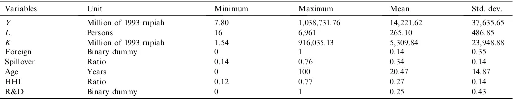
To construct a unique balanced panel data covering the se-lected period (1988–2000) and only for chemical and pharma-ceutical firms, this study follows several adjustment steps. A detailed explanation about data sources and the adjustment process is given at the beginning of the Appendix A. The ori-ginal observations for chemical and pharmaceutical firms (ISIC 35) in the selected period are 29,234 observations. After the adjustment process and the construction of a balanced pa-nel, the observations are reduced to 7,384 (consisting of 568 firms for 13 years). Some observations are removed during the adjustment of industrial codes and the cleaning of data from nonsense, noise, and missing values (Step 1 and Step 3 of the adjustments presented in Appendix A), some are dropped when choosing only ISIC 351 and 352 (Step 5), and some others are removed during the construction of a bal-anced panel (Step 6).16The largest numbers of observations are removed when choosing only ISIC 351 and 352 (17,962 out of 29,234 observations or 61.44%). Oil and gas refining sub-sectors (ISIC 353 and 354) are excluded from the dataset as these sub-sectors were not surveyed in 1988 and 1989. In addition, information regarding research and development (R&D) expenditure are available in the dataset since 1994. For the years 1988–93, the R&D dummy variable is defined as equal to that for the year 1994. The summary statistics for the main variables used in the econometric analysis are presented inTable A2.
6. ALTERNATIVE MODEL ESTIMATION AND ANALYSIS OF RESULTS
(a)Choosing the functional form
The first step in the SFA is to find an appropriate functional form that represents the data. Given the specifications of the
translogmodel in Eqn.(3), various sub-models of thetranslog
Table A1. Definitions of variables
Variables Definition
Production function
Y Value-added (in million rupiah), which is deflated using a wholesale price index of four-digit ISIC industries at a constant price of 1993
L Labor (number of workers)
K Capital (million rupiah), which is deflated using a wholesale price index of four-digit ISIC industries at a constant price of 1993
Inefficiency function
Foreign Foreign ownership, which is measured by a dummy variable: 1 if the share of foreign ownership is greater than 0%; and 0 if otherwise
Spillover Spillover variable, is measured by the share of foreign firms’ output over total output in three-digit ISIC industry Age Age of firms, is measured by the difference between year of survey and year of starting production
HHI Herfindahl–Hirschman index for a measure of concentration, which is calculated fromH¼Pm
i¼1S2i, forS
2
i is market share of each
firms
R&D Expenditure on research and development (R&D) is measured by dummy variable: 1 if firm spends on research and development activities during the observed years, and 0 otherwise
SpilloverHHI An interacting variable of spillover and HHI, which is a measure of productivity spillovers through concentration
SpilloverR&D An interacting variable of spillover and R&D dummy, which is a measure whether R&D firms receive more or less spillovers
are considered and tested under a number of null hypotheses. A null hypothesis ofbnt= 0 is to confirm whether Hicks-neu-tral technological progress is an appropriate specification for the dataset, while a null hypothesis of bt=btt=bnt= 0 is for no-technological progress in the production frontier. In addition, a null hypothesis of btt=bnt=bnk= 0, for all n andk, is to test for Cobb-Douglas production frontier and a null hypothesis of c=d0=dj= 0 is to confirm the no-inefficiency effect. For performing tests of the relevant null hypotheses, the generalized likelihood ratio statistic k=
2[l(H0)l(H1)] is employed, where l(H0) is the
log-likeli-hood value of the restricted frontier model, and l(H1) is the
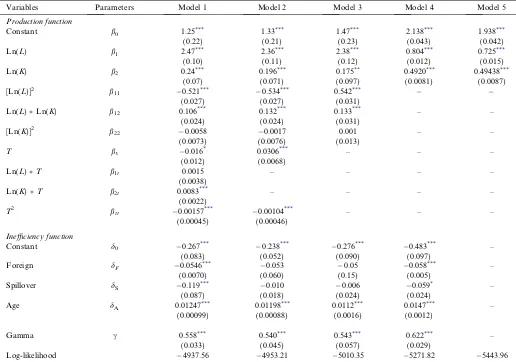
log-likelihood value of the translog model defined in Eqn. (3). If the null hypothesis is true, the test statistic has approx-imately av2distribution with degrees of freedom equal to the number of parameters involved in the restrictions. The test sta-tistic under the null hypothesis of no-inefficiency effects has approximately a mixedv2 distribution, and the critical value for this test is taken from Table 1 of Kodde and Palm (1986).17The estimation results fortranslogand the sub-mod-els under theBattese and Coelli’s (1995)SFA are presented in Table 4.
The last row of Table 4 presents log-likelihood values for each functional form. These log-likelihood values are used to calculate the generalized likelihood ratio statistic, k. The re-sults of the null hypotheses tests are presented inTable A3. From the results, it is apparent that various sub-models of thetranslogare found to be an inadequate representation of the data, given the specification oftranslogmodel. Therefore, the estimation results from Model 1 inTable 4are used in the interpretation of productivity spillovers.
(b)Foreign firms and productivity spillovers
The estimation results of a translog stochastic production frontier show that the coefficients of labor and capital have ex-pected positive signs. The positive and highly significant coef-ficients confirm the expected positive and significant output effects of labor and capital. In contrast, the squared variable of labor [(lnL)2] is negative and statistically significant at a
1% level, which indicates a diminishing return to labor. The same is not true of the squared capital. Its estimated coeffi-cient, while negative, turns out to be statistically insignificant. Furthermore, the estimated coefficient of the interacting vari-able between labor and capital (lnLlnK) is positive and significant at a 1% level, suggesting a substitution effect be-tween labor and capital.
For time variables, both coefficients of time (T) and its square are negative and statistically significant. A non-neutral technological progress toward capital is indicated by a positive and statistically significant (at 1% level) coefficient of the inter-acting variable between time and capital (TlnK). The com-bination of the various coefficients of variables that involveT
determines the movement of the production frontier over time, with this movement being positive (technological progress) or negative (technological regress) depending on values of K,L,
andT.18The results inTable 7below show that, when evalu-ated at the particular values ofK,L,andTfor each firm and time period, technological progress has been the dominant fac-tor contributing to productivity growth of both foreign and domestic firms in the Indonesian chemical and pharmaceutical industries over the full sample period.
A particular interest of this study is on the estimated coeffi-cients of the inefficiency function in the second part of Model 1 inTable 4. The negative and statistically significant (at 1% le-vel) coefficient of the dummy foreign ownership (Foreign) indicates that, on average, foreign firms achieve higher effi-ciency than their domestic counterparts do. Similarly, the average technical efficiency indices for both foreign and domestic firms confirm that foreign firms have higher technical efficiency than domestic firms during the observed years ( Fig-ure 1). The higher average efficiency indices of foreign firms compared to domestic firms also indicate that foreign firms are indeed premiers in the chemical and pharmaceutical sec-tors and operate on the technology frontier. This result sup-ports one of the classic hypotheses of the early literature in industrial organization, namely, that MNCs possess superior knowledge and efficiency, in the form of intangible assets, compared to their domestic counterparts.
The negative and significant coefficient on the spillover var-iable (spillover) in Model 1 in Table 4implies a positive and significant efficiency spillover in the chemical and pharmaceu-tical sectors. This result suggests that in the Indonesian chem-ical and pharmaceutchem-ical sectors higher foreign share results in domestic firms utilizing their resources in a more efficient way, which then leads to productivity gains. The evidence of posi-tive efficiency spillovers from FDI in this study is consistent with previous empirical studies on the Indonesian manufactur-ing sector which use a conventional approach of production function and focus on all manufacturing firms (e.g., Blalock & Gertler 2008; Sjoholm, 1999a).
The coefficient of a controlling variable, Age, is positive and statistically significant at a 1% level, indicating that older firms have higher inefficiency. This finding may not be a surprise, younger firms are likely to possess modern technology and capital equipment compared to older firms due to technology diffusion.
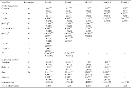
To ensure that the inclusion of foreign firms in the estima-tion on FDI spillovers does not introduce bias, this study esti-mates also the frontier for only domestic firms. The results are presented inTable A4. Interestingly, all coefficients have sim-ilar signs and levels of significance as those for the sample of all firms. This is not a surprise given a fact that foreign firms are only 14.98% of the total sample (1,106 out of 7,384 obser-vations). The negative and highly significant coefficient of the key variable, spillovers, is consistent with the result for the Table A2. Summary statistics
Variables Unit Minimum Maximum Mean Std. dev.
Y Million of 1993 rupiah 7.80 1,038,731.76 14,221.62 37,635.65
L Persons 16 6,961 265.10 486.85
K Million of 1993 rupiah 1.54 916,035.13 5,309.84 23,948.88
Foreign Binary dummy 0 1 0.14 0.35
Spillover Ratio 0.14 0.76 0.34 0.14
Age Years 0 100 20.47 14.87
HHI Ratio 0.12 0.77 0.27 0.14
R&D Binary dummy 0 1 0.25 0.43
sample of all firms, suggesting that the finding of positive FDI spillovers on technical efficiency of domestic firms inTable 3is not simply a result of biased estimation. FollowingKathuria (2000), this study chooses to proceed with the sample of all firms since it measures inefficiency from a distance to the most efficient firms, which can be either foreign or domestic firms. Hence, the inefficiency indexes are measured relative to the best-practice foreign or domestic firms.
Considering that the shock in the economic environment, such as economic crisis, might be affecting FDI spillovers, this
study also estimates the samples for the period before the crisis (1988–96) and for the period after the crisis (1997–2000). The estimation results for these two periods are presented inTable A5. In both periods, the coefficients of spillovers are negative. However, the significance levels are different; it is significant at the 1% level for the before-crisis period but it is marginally sig-nificant at the 10% level for the crisis period. In addition, the coefficient is smaller for the crisis period compared to the be-fore-crisis period, suggesting that the magnitude of spillovers is smaller during the crisis period. However, the short time Table 4. Maximum likelihood estimates of stochastic production frontier
Variables Parameters Model 1 Model 2 Model 3 Model 4 Model 5
Production function
Constant b0 1.25*** 1.33*** 1.47*** 2.138*** 1.938***
(0.22) (0.21) (0.23) (0.043) (0.042) Ln(L) b1 2.47*** 2.36*** 2.38*** 0.804*** 0.725***
(0.10) (0.11) (0.12) (0.012) (0.015) Ln(K) b2 0.24*** 0.196*** 0.175** 0.4920*** 0.49438***
(0.07) (0.071) (0.097) (0.0081) (0.0087) [Ln(L)]2 b
11 0.521*** 0.534*** 0.542***
(0.027) (0.027) (0.031)
Ln(L)Ln(K) b12 0.106*** 0.132*** 0.133*** – –
(0.024) (0.024) (0.031) [Ln(K)]2 b
22 0.0058 0.0017 0.001 – –
(0.0073) (0.0076) (0.013)
T bt 0.016* 0.0306*** – – –
(0.012) (0.0068)
Ln(L)T b1t 0.0015 – – – –
(0.0038)
Ln(K)T b2t 0.0083*** – – – –
(0.0022)
T2 btt 0.00157*** 0.00104*** – – – (0.00045) (0.00046)
Inefficiency function
Constant d0 0.267*** 0.238*** 0.276*** 0.483*** –
(0.083) (0.052) (0.090) (0.097)
Foreign dF 0.0546*** 0.053 0.05 0.058*** –
(0.0070) (0.060) (0.15) (0.005)
Spillover dS 0.119*** 0.010 0.006 0.059* –
(0.087) (0.018) (0.024) (0.024)
Age dA 0.01247*** 0.01198*** 0.0112*** 0.0147*** –
(0.00099) (0.00088) (0.0016) (0.0012)
Gamma c 0.558*** 0.540*** 0.543*** 0.622*** – (0.033) (0.045) (0.057) (0.029)
Log-likelihood 4937.56 4953.21 5010.35 5271.82 5443.96 Note: Model 1 is atranslogproduction function. Models 2 and Model 3 represent a Hicks-neutral and a no-technological progress production functions, respectively. Model 4 is a Cobb–Douglas production function and Model 5 represents a no-inefficiency production function. Standard errors are in parentheses and presented until two significant digits, and the corresponding coefficients are presented up to the same number of digits behind the decimal points as the standard errors.
*Denotes significance at 10%. **Denotes significance at 5%. ***
Denotes significance at 1%.
Table A3. Tests of hypothesis of stochastic production frontier
Test H0 k v21% Conclusion
Hicks neutral bnt= 0 31.30 9.210 Hicks neutral rejected No-technological progress bt=bnt=btt= 0 145.58 13.277 No-technological progress rejected Cobb–Douglas bnk=bt=bnt=btt= 0 668.52 18.475 Cobb–Douglas rejected No-inefficiency c=d0=dj= 0 1012.80 17.755 No-inefficiency rejected
Source: Authors’ calculation from log-likelihood functions.
span for the sample of the crisis period means that the results need to be treated with caution as there are substantially fewer observations than for the full period or the pre-crisis period.
(c)Productivity spillovers and competition
This section tests H2 that productivity spillovers are affected by the degree of competition. The Herfindahl–Hirschman
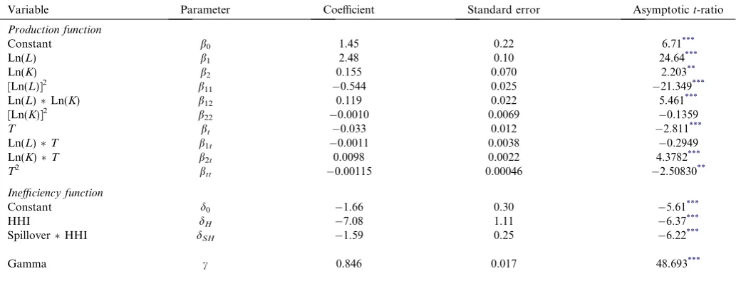
In-dex(HHI) is used as a measure of the degree of competition within three-digit ISIC industries (a higher value of HHI indi-cates greater concentration of sales among producers). Higher concentration is an inverse measure of static competition that can protect inefficient firms. However, higher concentration can also be the result of dynamic competition among firms of differential efficiency that removes inefficient firms from the industry as argued by Demsetz (1973) and Peltzman (1977). The first argument suggests that HHI is associated with greater inefficiency, while the latter argument suggests that HHI is associated with lower inefficiency. The estimated maximum likelihood parameters of a stochastic production function for productivity and competition are presented in Ta-ble 5. The spillover variable without interacting with HHI is excluded from the estimation because of multicollinearity with the interacting variable.
Each estimated parameter of production functions shown in Table 5has a similar sign and significance as in the baseline model shown inTable 4. Therefore, there is no need to explain the estimated parameters of production function further. In the inefficiency function, the negative coefficient of competi-tion (HHI) indicates that concentracompeti-tion among firms in the Indonesian chemical and pharmaceutical sectors decreases the inefficiency of firms, which is consistent with the argument
0.94 0.95 0.96 0.97
1988 1989 1990 1991 1992 1993 1994 1995 1996 1997 1998 1999 2000
TE Foreign Firms TE Domestic Firms
Figure 1.Average technical efficiency indexes of foreign and domestic firms.
Table A4. Maximum likelihood estimates of stochastic production frontier for domestic firms
Variables Parameters Model 1 Model 2 Model 3 Model 4 Model 5
Production function
Constant b0 1.48*** 1.37*** 1.59*** 2.119*** 2.107***
(0.22) (0.21) (0.21) (0.036) 0.044 Ln(L) b1 1.92*** 1.95*** 1.95*** 0.858*** 0.760***
(0.11) (0.11) (0.11) (0.014) 0.016 Ln(K) b2 0.314*** 0.317*** 0.274*** 0.4474*** 0.4435***
(0.072) (0.071) (0.070) (0.0082) 0.0095 [Ln(L)]2 b
11 0.569*** 0.556*** 0.607*** – –
(0.027) (0.028) (0.023)
Ln(L)Ln(K) b12 0.232*** 0.223*** 0.259*** – –
(0.023) (0.023) (0.020)
[Ln(K)]2 b22 0.0339*** 0.0311*** 0.0326*** – –
(0.0074) (0.0074) (0.0069)
T bt 0.005 0.0317*** – –
(0.013) (0.0067)
Ln(L)T b1t 0.0043 – – – –
(0.0039)
Ln(K)T b2t 0.0031 – – – –
(0.0024) T2 btt 0.00147***
0.00127*** – – –
(0.00047) (0.00047)
Inefficiency function
Constant d0 0.562*** 0.565*** 1.05*** 1.28*** –
(0.096) (0.077) (0.19) (0.26)
Spillover dS 0.44*** 0.49*** 0.53*** 0.62*** –
(0.15) (0.12) (0.15) (0.21)
Age dA 0.1611*** 0.0164*** 0.0208*** 0.0247*** –
(0.0015) (0.0012) (0.0023) (0.0031)
Gamma c 0.552*** 0.615*** 0.679*** 0.754*** –
(0.043) (0.029) (0.036) (0.029)
Log-likelihood 3979.40 3983.45 4023.07 4235.33 4419.20
No. of observations 6,278 6,278 6,278 6,278 6,278 Note: Model 1 is atranslogproduction function. Models 2 and Model 3 represent a Hicks-neutral and a no-technological progress production function, respectively. Model 4 is a Cobb–Douglas production function and Model 5 represents a no-inefficiency production function. Standard errors are in parentheses and presented until two significant digits, and the corresponding coefficients are presented up to the same number of digits behind the decimal points as the standard errors.
***Denotes significance at 1%.
that concentration is a result of dynamic competition that re-moves inefficient firms.
The negative coefficient of the interacting variable between concentration and spillovers (HHISpillovers) suggests that higher concentration is associated with larger spillovers from foreign presence. From these findings, it may be inferred that domestic firms operating in a concentrated sub-sectors of the Indonesian chemical and pharmaceutical sectors may gain spillover benefits from foreign firms. This finding is consistent with the findings byBlomstrom and Sjoholm (1999) and Sjo-holm (1999b) on the overall Indonesian manufacturing.
Although the present study differs with those two previous studies in terms of the methodology, data techniques, and per-iod of observations, the findings of this present study can be seen as a support and update evidence of those two previous studies.
(d)Productivity spillovers and absorptive capacity
The estimated parameters of productivity spillovers and absorptive capacity are presented in Table 6. The focus of analysis is on the estimated parameters of the inefficiency Table A5. Estimates for the periods before crisis and after crisis
Variables Parameters Before crisis (1988–96) After Crisis (1997–2000)
Coefficient SE Coefficient SE
Production function
Constant b0 0.30 0.33 4.62*** 1.22
Ln(L) b1 2.53*** 1.41 2.51*** 0.43
Ln(K) b2 0.53*** 0.12 0.44** 0.23
[Ln(L)] b11 0.516*** 0.043 0.619*** 0.050
Ln(L)Ln(K) b12 0.077* 0.042 0.318*** 0.040
[Ln(K)]2 b
22 0.020 0.016 0.031 0.018
T bt 0.001 0.021 0.23 0.20
Ln(L)T b1t 0.0231*** 0.0074 0.083 0.026 Ln(K)T b2t 0.0073* 0.0042 0.053 0.012
T2 btt 0.0019 0.0012 0.003 0.008
Inefficiency function
Constant d0 0.188*** 0.066 0.271*** 0.050
Foreign dF 0.052*** 0.0073 0.098*** 0.012 Spillover dS 0.052*** 0.021 0.0074* 0.0040 Age dA 0.01174*** 0.00094 0.0047*** 0.0013
Gamma c 0.541*** 0.076 0.304*** 0.112
Log-likelihood 3420.79 2381.85
No. of observations 5,112 2,272
Note: Standard errors are presented until two significant digits and the corresponding coefficients are presented up to the same number of digits behind the decimal points as the standard errors.
*Denotes significance at 10%. **Denotes significance at 5%. ***Denotes significance at 1%.
Table 5. Maximum likelihood estimates of stochastic production frontier with inefficiency coefficients as a function of HHI and SpilloverHHI Variable Parameter Coefficient Standard error Asymptotict-ratio
Production function
Constant b0 1.45 0.22 6.71***
Ln(L) b1 2.48 0.10 24.64***
Ln(K) b2 0.155 0.070 2.203**
[Ln(L)]2 b
11 0.544 0.025 21.349***
Ln(L)Ln(K) b12 0.119 0.022 5.461***
[Ln(K)]2 b
22 0.0010 0.0069 0.1359
T bt 0.033 0.012 2.811***
Ln(L)T b1t 0.0011 0.0038 0.2949
Ln(K)T b2t 0.0098 0.0022 4.3782***
T2 btt 0.00115 0.00046 2.50830**
Inefficiency function
Constant d0 1.66 0.30 5.61***
HHI dH 7.08 1.11 6.37***
SpilloverHHI dSH 1.59 0.25 6.22***
Gamma c 0.846 0.017 48.693***
Note: Figures are rounded. Standard errors are presented until two significant digits and the corresponding coefficients andt-ratio are also presented up to the same number of digits behind the decimal points as the standard errors.
**Denotes significance at 5%. ***
Denotes significance at 1%.
function (the middle part ofTable 6). The coefficient of the re-search and development dummy (R&D) is negative and signif-icant at the 1% level, suggesting that firms with R&D expenditure, on average, have higher efficiencies compared to those without R&D expenditure. This finding is similar to that ofTodo and Miyamoto’s (2006)study of the overall Indo-nesian manufacturing sector.
The negative coefficient of the interacting variable between R&D and spillovers (R&DSpillover) suggests that firms with R&D expenditure gain more spillovers from foreign firms. Given this result, it is possible to infer that firms with R&D expenditure can reap benefits from foreign firms’ presence by upgrading their knowledge and creating new inno-vation. This finding confirms that firms’ absorptive capacity (or firms’ specific characteristic) determines productivity
spill-overs from FDI, as argued in some previous studies, for exam-ple, byKathuria (2000, 2001). This finding is also in line with the finding byTakii (2005)for the whole Indonesian manufac-turing firms, even though this present study includes also the period of economic crisis in the estimation.
(e)Sources of productivity growth and FDI spillovers
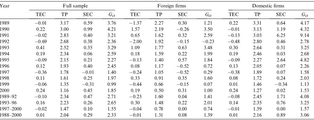
The indices of TEC;TP;SEC andGO are calculated using
Eqns.(7)–(14)and the average of these indices for the selected period is presented inTable 7. It is apparent fromTable 7that TEC;TP;SEC andGOfor domestic firms are on average
high-er than those for foreign firms. These results suggest that domestic firms are catching up the foreign firms in terms of technical efficiency, technology, and scale efficiency. With Table 6. Maximum likelihood estimates of stochastic production frontier with inefficiency coefficient as a function of R&D and SpilloverR&D Variable Parameter Coefficient Standard error Asymptotict-ratio
Production function
Constant b0 1.24 0.21 5.92***
Ln(L) b1 2.392 0.097 2.454**
Ln(K) b2 0.278 0.065 4.244***
[Ln(L)] b11 0.559 0.026 21.179***
Ln(L)Ln(K) b12 0.140 0.022 6.348***
[Ln(K)]2 b
22 0.0163 0.0066 2.4354**
T bt 0.024 0.012 1.975*
Ln(L)T b1t 0.0017 0.0037 0.4709
Ln(K)T b2t 0.0100 0.0021 4.7205***
T2 btt 0.00157 0.00045 3.50424***
Inefficiency function
Constant d0 0.45 0.17 2.63***
R&D dR 0.466 0.063 7.418***
SpilloverR&D dSR 0.46 0.19 2.40**
Gamma c 0.588 0.044 13.284***
Note: Figures are rounded. Standard errors are presented until two significant digits and the corresponding coefficients andt-ratio are also presented up to the same number of digits behind the decimal points as the standard errors.
*Denotes significance at 10%. **Denotes significance at 5%. ***
Denotes significance at 1%.
Table 7. Sources of productivity growth
Year Full sample Foreign firms Domestic firms
TEC TP SEC GO TEC TP SEC GO TEC TP SEC GO
1989 0.01 3.17 0.59 3.76 1.37 2.27 0.30 1.21 0.22 3.31 0.64 4.17 1990 0.22 3.00 0.99 4.21 1.57 2.19 0.26 3.50 0.01 3.13 1.19 4.32 1991 0.02 2.83 0.40 3.21 0.65 1.62 0.32 2.59 0.13 3.03 6.25 9.14 1992 0.69 2.68 0.38 2.36 2.00 1.92 0.15 0.23 0.48 2.80 0.46 2.78 1993 0.41 2.52 0.35 3.29 1.09 1.77 0.63 3.48 0.30 2.64 0.31 3.25 1994 0.19 2.34 0.06 2.59 0.18 1.59 0.22 1.99 0.19 2.46 0.03 2.68 1995 0.09 2.15 0.21 2.27 0.13 1.40 0.57 1.84 0.09 2.27 2.64 4.82 1996 0.12 1.93 0.40 2.45 0.08 1.17 0.52 0.72 0.13 2.05 0.07 2.26 1997 0.36 1.78 0.01 1.40 0.24 1.05 0.52 0.29 0.38 1.89 0.07 1.58 1998 0.11 1.61 0.25 1.97 0.33 0.91 0.35 1.60 0.08 1.72 0.24 2.03 1999 0.06 1.35 0.31 0.99 0.44 0.66 0.15 0.07 0.01 1.46 0.34 1.13 2000 0.24 1.16 0.45 1.85 0.19 0.50 0.31 1.00 0.24 1.27 0.02 1.53 1989–92 0.10 2.34 0.47 2.71 0.23 1.60 0.04 1.41 0.08 2.45 1.71 4.08 1993–96 0.16 2.23 0.26 2.65 0.30 1.48 0.22 2.01 0.14 2.35 0.76 3.25 1997–2000 0.02 1.47 0.10 1.55 0.04 0.78 0.00 0.74 0.01 1.59 0.00 1.57 1988–2000 0.01 2.04 0.29 2.33 0.01 1.31 0.08 1.39 0.01 2.16 0.89 3.06 Note: Arithmetic average of annual rate in percentage.
Source: Authors’ calculation using Eqns.(7)–(14).
larger TEC indices of some domestic firms than those of foreign firms, all domestic firms are likely to approach the same level of technical efficiency as achieved by foreign firms in the long run. The same result would also turn out to be for technology level and scale efficiency. As the indices of TP for domestic firms are, on average, larger than those for foreign firms therefore domestic firms may eventually approach to the same level of technology as achieved by foreign firms. Scale efficiency may also be approaching the same level for domestic and foreign firms.
Table 7also shows that the major contribution to productiv-ity growth in the Indonesian chemical and pharmaceutical firms is from technological progress. This is not surprising as chemical and pharmaceutical sectors are capital- and technol-ogy-intensive. Furthermore, when the sample is divided into domestic and foreign firms, technological progress is the major driver of productivity growth in both groups. In contrast, the TEC and SEC indices are relatively constant, suggesting that these two components do not contribute much to productivity growth.
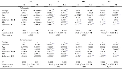
Using the indexes of TEC, TP, SEC, andGOobtained from the decomposition, we then estimate the impact of FDI spill-overs on total factor productivity (TFP) growth and its sources. The estimated parameters are presented in Table 8. We perform both random effect (RE) and fixed effect (FE) pa-nel data models for TFP growth and its sources. The Haus-man specification test is used to choose which of the two models is better at representing the data. It can be seen from the probability forv2-statistic of the Hausman test (Table 8)
that the RE model is preferred for TEC and SEC, but the FE model is better for TP andGOin all samples. For the sam-ple of domestic firms only, RE model turns out to be a better model for TEC and FE model is well suited for TP, TEC, and
GO. Therefore, the interpretation of the estimated parameters for TFP growth and its sources is based on the best-suited model in each case.
Table 8 reveals that FDI spillovers contribute signifi-cantly to technological progress (as shown by a positive and significant estimate of spillover variable in the regres-sion on technological progress). However, spillovers do not contribute much to technical efficiency and scale effi-ciency (as shown by a statistically insignificant estimate of spillover variable on technical efficiency change and scale efficiency change). These results indicate the role of technol-ogy transfers in generating productivity spillovers. Hence, one may argue that the spillover effects of productivity growth in the Indonesia chemical and pharmaceutical firms are predominantly due to enhancing technological progress and not as a result of technical efficiency and scale effi-ciency improvements.
Moreover, a positive and statistically significant estimate of concentration on technological progress suggests that a more competitive environment may reduce technological progress. A positive and significant estimate is also found for R&D dummy, which indicates that firms with R&D expenditure have higher technological progress than those without R&D expenditure. The positive and statistically significant estimate of interacting variable between spillover and R&D indicates
Table 8. Sources of productivity growth and FDI spillovers
TEC TP SEC GO
FE RE FE RE FE RE FE RE
Full sample
Foreign 0.0015 0.000093 0.0012** 0.0033*** 0.058 0.0071 0.062 0.0018
Spillover 0.013 0.0037 0.0057*** 0.036*** 0.068 0.035 0.088* 0.047*
Age 0.000095 0.000013 0.0018*** 0.00093*** 0.0043** 0.00092 0.0065*** 0.00087***
HHI 0.0060 0.010 0.0083*** 0.038*** 0.26 0.043 0.28 0.010 SpilloverHHI 0.0052 0.0071 0.011*** 0.029*** 0.12 0.0052 0.14 0.062 RD 0.0012 0.000043 0.00031* 0.0022*** 0.12*** 0.11*** 0.13*** 0.12*** SpilloverRD 0.0017 0.00050 0.00057* 0.0076***
0.27***
0.26*** 0.29***
0.27***
R2 0.001 0.001 0.006 0.048 0.001 0.005 0.001 0.005 Hausman test Probv2= 0.847: RE Probv2= 0.000: FE Probv2= 0.267: RE Probv2= 0.016: FE
Observations 6,816 6,816 6,816 6,816
Domestic firms
Foreign – – – – – – – –
Spillover 0.012 0.0036 0.0063*** 0.038*** 0.040 0.035 0.059* 0.050*
Age 0.000083 0.000011 0.0019*** 0.00095*** 0.0050 0.0010 0.0072*** 0.00096***
HHI 0.0085 0.011 0.0076*** 0.039*** 0.28 0.052 0.30 0.00063
SpilloverHHI 0.0026 0.0086 0.011*** 0.030*** 0.085 0.0012 0.10 0.055
RD 0.0016 0.00017 0.000057* 0.0021*** 0.14*** 0.13*** 0.15*** 0.14***
SpilloverRD 0.0028 0.000026 0.0010* 0.0067*** 0.31** 0.31*** 0.33*** 0.32***
R2 0.001 0.001 0.004 0.041 0.001 0.005 0.001 0.005 Hausman test Probv2= 0.808: RE Probv2= 0.000: FE Probv2= 0.000: FE Probv2= 0.016: FE
Observations 5,856 5,856 5,856 5,856
Source: Authors’ estimation using STATA10. FE is fixed-effect model and RE is random-effect model. Coefficients are presented until two significant digits.
*Denotes significant at 10% level. **Denotes significant at 5% level. ***Denotes significant at 1% level.
that firms with R&D expenditure tend to gain more technolog-ical spillovers. However, the estimate for an interacting vari-able between spillover and concentration is negative and statistically significant, suggesting that competition is associ-ated with higher spillovers on technological progress.
Endogeneity is a particularly important issue for the key variable, spillover. The OLS coefficients shown in Table 8 are estimated under an assumption that the variation in the spillover variable is exogenous to the productivity growth of domestic firms. If this assumption is not fulfilled then OLS may yield biased estimates. In the case where FDI is attracted to industries (or sub-sectors) with high productivity growth, the estimates shown inTable 8could be biased upward. Alter-natively, foreign firms may be attracted to slow-growing industries in order to gain a greater competitive advantage, which in this case, the OLS estimates shown inTable 8may bias downward.
In dealing with this possible endogeneity bias, this study pursues two strategies, followingHaskel, Pereira, and Slaugh-ter (2007). The first strategy is to use lagged measures of spill-over instead of spillspill-over at timet. Lags may be appropriate because spillovers may take time to materialize. The second strategy is to adopt an instrumental variable estimation, as an alternative to OLS. This study employs the Arellano-Bond GMM estimator, which adds a lagged dependent variable and once-lagged independent variables as instrumental variables.
The estimation results for the first and the second strategies of addressing endogeneity bias are presented inTable 9. For the first strategy, we present the results of the best-suited mod-el. As the results show, the signs and significances of the lagged spillover (Spillovert1) on productivity growth (and its
sources) are similar to those of spillover at timetshown in Ta-ble 8. The only notable difference is the value of the coeffi-cients, which are larger for the lagged spillover. The positive
and significant coefficient Spillovert1onGOis consistent with the spillover-taking-time argument. The positive and signifi-cant coefficient Spillovert1on TP, and positive and
insignifi-cant on TEC and SEC, suggest that the presence of FDI contributes significantly to technological progress but not to technical efficiency change and scale efficiency change.
The results for the second strategy are presented in the lower part ofTable 9. The Arellano–Bond GMM estimates on spill-over present similar conclusions as those ofTable 8. By adding a lagged dependent variable and once-lagged variables as instruments, the results show a positive and significant affect of spillover on productivity growth and technological progress. However, the level of significance of the coefficient on technological progress in this model is lower than those shown inTable 8, which may be due to the lack of good instru-ments.
7. CONCLUSION AND POLICY IMPLICATIONS
This study examines the productivity spillovers from FDI in the Indonesian chemical and pharmaceutical sectors by using a unique and extensive firm-level panel data covering the per-iod 1988–2000. Unlike most of the previous studies on FDI productivity spillovers, this paper uses the stochastic frontier production function following Battese and Coelli (1995)and a generalizedMalmquist output-oriented index to decompose productivity growth. The intra-industry productivity spillovers are examined through the spillover variable, and the roles of competition and R&D in extending spillovers from FDI are evaluated to test a channel of productivity spillovers.
The empirical results show that intra-industry productivity spillovers are present in the Indonesian chemical and pharma-ceutical sectors. It also shows that competition facilitates Table 9. Sources of productivity growth and FDI spillovers: dealing with endogeneity
TEC TP SEC GO
Strategy 1: Replacing spillover with a lagged-spillover Full sample
Spillovert1 0.00079 0.0010*** 0.027 0.0031*
R2 0.001 0.007 0.005 0.001
Hausman test Probv2= 0.456: RE Probv2= 0.000: FE Probv2= 0.282: RE Probv2= 0.023: RE
Observation 6,816 6,816 6,816 6,816
Domestic firms
Spillovert1 0.00020 0.00018*** 0.026 0.0030*
R2 0.001 0.004 0.005 0.001
Hausman test Probv2= 0.849: RE Probv2= 0.000: FE Probv2= 0.157: RE Probv2= 0.010: FE
Observation 5,856 5,856 5,856 5,856
Strategy 2: Arellano–Bond GMM estimations Full sample
Spillover 0.031 0.0033* 0.012 0.015*
Wald-v2 Probv2= 0.000 Probv2= 0.000 Probv2= 0.064 Probv2= 0.000
Observation 5,680 5,680 5,680 5,680
Domestic firms
Spillover 0.035 0.00097* 0.037 0.039*
Wald-v2 Probv2= 0.000 Probv2= 0.000 Probv2= 0.073 Probv2= 0.017
Observation 4,859 4,859 4,859 4,859
Source: Authors’ estimation using STATA10.
Note: FE is fixed-effect model and RE is random-effect model. The estimation for all sample includes Foreign, Age, HHI, HHISpillover, RD, and RDSpillover variables; the estimation for domestic firms includes Age, HHI, HHISpillover, RD, and RDSpillover variables. Coefficients are presented until two significant digits.
*Denotes significant at 10% level. ***Denotes significant at 1% level.