www.elsevier.nl / locate / econbase
Cooperation and noise in public goods experiments:
applying the contribution function approach
a ,* b
Jordi Brandts , Arthur Schram
a
´ ´
Instituto de Analisis Economico(CSIC), Campus UAB, 08193 Bellaterra, Barcelona, Spain
b
CREED, Department of Economics, University of Amsterdam, Amsterdam, The Netherlands
Received 30 June 1998; received in revised form 31 July 1998; accepted 31 October 1999
Abstract
We introduce a new design for experiments with the voluntary contributions mechanism for public goods. Subjects report a complete contribution function in each period, i.e. a contribution level for various marginal rates of transformation between a public and a private good. The results show that subjects’ behavior cannot be explained exclusively as the result of errors. Individuals exhibit essentially one of two types of behavior. One group of subjects behaves in a way consistent with some kind of other-regarding motivation. Some features of the data indicate that these subjects’ behavior is interdependent. Another group of subjects behaves in accordance with a utility function that depends only on their own earnings. The interaction between these two groups may be important when explaining behavior over time. 2001 Elsevier Science B.V. All rights reserved.
Keywords: Experimental economics; Public goods games; Cooperation
JEL classification: C90; C91; D63
1. Introduction
A long stream of laboratory experiments has studied voluntary contributions in public goods environments and established one basic fact: subjects contribute to the provision of the public good in situations in which it is a dominant strategy not
*Corresponding author. Tel.: 134-93-580-6612; fax: 134-93-580-1452. E-mail address: [email protected] (J. Brandts).
to do so. This result has been obtained in a rather large number of experimental frameworks by researchers coming from different traditions. Ledyard (1995) presents an excellent survey of this literature.
While the contribution result has by now been solidly established, there is, at this point, no agreement about why subjects contribute. There are basically two types of explanations. One general view is that at least some subjects are guided by some kind of cooperative or altruistic motives. They contribute to the public good either because they derive additional utility from it or because they are somehow able to tacitly cooperate to reach an outcome that yields higher payoffs to them than the no-contribution equilibrium.
A different type of explanation conjectures that subjects’ lack of familiarity with the game, together with a specific feature of the standard experimental design, leads to behavior which may be incorrectly interpreted as voluntary contributions. In the most standard experimental set-up, a linear public goods game (hereafter lpgg), the dominant strategy Nash equilibrium corresponds to zero contributions. The only possible ‘mistake’ a subject can make in this ‘corner’ situation is to contribute too much to the public good. According to this view, these mistakes can then be misinterpreted as purposeful contributions.
The possibility of mistakes being the explanation of observed contributions has recently been investigated experimentally by Palfrey and Prisbrey (1996). They present some lpgg experiments specifically designed to analyze whether subjects contribute just by mistake. In these experiments, subjects are not faced with the same relative prices or marginal rates of transformation (hereafter mrt) between
1
the private and the pure public good throughout the different periods. Instead, in every period the mrt is independently drawn for each individual. The mrt can take a range of different values. For some values of the mrt contributing nothing to the public good is the dominant strategy, while for other values the dominant strategy is to contribute everything to the public good. The variation of the mrt across periods generates data about decisions in different situations. According to Palfrey and Prisbrey the results from their experiments can be explained by the mistakes interpretation of positive contributions.
The idea that observed behavior can be explained by a combination of errors and some kind of ‘non-selfish’ motivation is central in both the models of Anderson et al. (1998) and Palfrey and Prisbrey (1997). In the former paper, an equilibrium model is presented in which altruism and errors determine contribution behavior. The kind of altruism chosen is the linear form discussed by Ledyard
2
(1995). Anderson et al. (1998) derive a unique equilibrium density of contribu-tions for this kind of altruism and a logistic form of the error distribution. They show that the (comparative statics) predictions of this model are in line with
1
Palfrey and Prisbrey (1996) used the term ‘marginal rate of substitution’, but ‘marginal rate of transformation’ as well as ‘relative prices’ would appear to be more appropriate terms.
2
typical results from public good experiments. Palfrey and Prisbrey (1997) use the same design as in their previous paper. They present a model that allows for errors, linear altruism and ‘warm glow’. The last term, introduced by Andreoni (1990), is meant to capture the utility that individuals derive from the act of contributing per se. Palfrey and Prisbrey estimate the parameters of their model
3
and find evidence for errors and warm glow, but not for linear altruism.
Whereas the combination of errors with some kind of non-selfish behavior assumed in Anderson et al. (1998) and Palfrey and Prisbrey (1997) may be a valid approach, the elaboration of the non-selfish part is still open for discussion. What warm glow feelings and linear altruism have in common is that, for lpgg games, they yield the prediction that behavior will be independent of the behavior of others. It is possible, however, that interdependence is a necessary ingredient of a satisfactory explanation of people’s behavior.
Other models predict that subjects’ choices will depend on others’ behavior or on expectations about their behavior, in a variety of ways. Rabin (1993) presents a theoretical model in which individuals’ behavior depends on others’ intentions: people want to help those who want to help them and hurt those who want to hurt them. Levine (1998) develops a model of reciprocal altruism where the weight attributed to others’ income depends on what the others’ level of altruism is believed to be. He finds support for the model in data from various kinds of experiments, including lpggs. Bolton and Ockenfels (2000) and Fehr and Schmidt (1999) present two related distributional models in which individuals are in-fluenced by different variations of inequality aversion; it is this aversion that leads to interdependence. In Brandts and Schram (1996) we present a model where subjects with a particular motivation, which we call cooperative gain seeking, are willing to forgo the gains from individual deviation by contributing to a public good. A subject of this type will do so if and only if (s)he expects that the level of contributions by other subjects of this type is high enough to make earnings higher than if none of them contributed anything. Current experimental research is directed at exploring the relevance of different types of interdependence.
In this paper we attempt to take the study of voluntary contributions to public goods one step further. We present a new design for lpgg experiments and analyze the results in order to obtain better information about the importance of errors and
4
the type of non-selfish behavior exhibited by subjects. In our design, subjects are
3
Keser (1996) and Sefton and Steinberg (1996) study experimental games with a dominant strategy in the interior of the strategy space. They observe significant over-contributions. Anderson et al. (1998) argue that even this may be explained by a proper modeling of errors in decision making, however.
4
requested to supply a complete ‘contribution function’ in every period; they have to decide a priori on their contribution level for different possible mrts. Then one of the mrts is randomly selected and the effective contribution of the individual is the one corresponding to the selected mrt.
We believe that this design presents a number of advantages over other designs used in previous experimental work in this area. It yields very rich information about individual behavior, since in every period every subject makes a number of decisions equal to the number of different mrts. In addition, we chose the different values of the mrt in such a way that in every period every individual has to make decisions about three kinds of situations: in some situations it is a dominant strategy and efficient to contribute everything to the public good, in some other situations it is a dominant strategy to contribute nothing, although it is efficient for everybody to contribute everything, and in a third kind of situation it is a dominant strategy to contribute nothing and it is also efficient to do so.
The extensive data-set together with the distinct situations with respect to dominance and efficiency provided by our design will allow us to draw three major conclusions. First, errors alone cannot explain contributions in our lpgg. Second, subjects’ behavior is diverse. Third, the behavior of a group of subjects is sensitive to the choices of others, i.e. their behavior is interdependent.
This paper is organized as follows. In Section 2 we present the experimental procedures and design. Sections 3 and 4 present our aggregate and individual results. Section 5 presents a closer look at and interpretation of the results, highlighting the evidence of interdependent behavior. Section 6 contains a summary and some conclusions.
2. Experimental procedures and design
Our experiment consisted of various treatments, each of which was run twice: once at the CREED laboratory at the University of Amsterdam and once at the
5
LEEX laboratory at the Pompeu Fabra University in Barcelona. The subject pool consisted of the undergraduate population at both institutions. In each session, 13 subjects were brought into the laboratory and randomly appointed seats. They were separated by partitions and no communication was allowed. One subject was randomly chosen to be a monitor and assisted with the random draws in the experiment. Instructions were computerized (see Appendix A for a translation) and could be read at one’s own pace. After subjects had finished reading the instructions, two practice periods were run, in which it was made clear that there was no interaction: the computer randomly determined the ‘decisions of other
5
6
individuals’. The experiment itself was computerized and consisted of 10
7
consecutive periods.
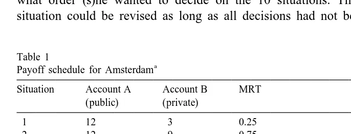
In each period, subjects were anonymously allocated to three groups of four. They were asked to divide 9 tokens by investing each in one of two accounts, denoted by A and B. A was a group account yielding an identical amount of money to every member of the group. B was a private account yielding money to the subject alone. This division had to be made for 10 different ‘situations’, in which the payoff to the public account was kept constant, but the payoff to the private account varied. Table 1 gives an overview of the values used in the
8
Amsterdam experiments. In Barcelona the same mrts were used.
This payoff schedule was presented in tabular form on a handout, on an overhead projector, and on the computer screen. Each subject could determine in what order (s)he wanted to decide on the 10 situations. The decision for any situation could be revised as long as all decisions had not been finalized. After
Table 1
a
Payoff schedule for Amsterdam
Situation Account A Account B MRT (public) (private)
The numbers are the payoff per token, in Dutch cents. To obtain the numbers for Barcelona in pesetas, we used the exchange rate PTA 15FL 0.015. The mrt is defined as the value for an individual of a token invested in the private account divided by the value for an individual of a token invested in the public account.
6
The software was developed by CREED programmer Otto Perdeck. Versions in English, Spanish and Dutch are available on request.
7
It is standard practice to run multiple periods in this kind of environment. As will be discussed in Section 4, in our case the multiple-period procedure served a specific purpose, since behavior over time will allow us to investigate the presence of interdependence in subjects’ motivation.
8
each individual had finalized the division of tokens for all situations, one situation was randomly selected to be played. How this was done is described below. Then, the experiment proceeded to the next period.
Three treatments were studied: homogeneous vs. heterogeneous situations, partial vs. full information and partners vs. strangers. The first two treatments were introduced to control for some possible effects of our design. Ledyard (1995) suggests that contributions to the public good in a lpgg may be affected by the level of heterogeneity in the environment. In our design we have to draw one of the mrts at random to determine payment. We need to control for the possible effect of the difference in heterogeneity between the two ways one can do this, per individual or per group. In our ‘heterogeneous treatment’, a situation (i.e. the mrt) was chosen separately for each individual. Thus, in general, the decisions by which the total investment in the group account and the individual payoffs were determined were based on different mrts for different subjects. In the ‘homoge-neous treatment’, the monitor selected one situation per group. Thus, the investments in the group account and the payoffs were determined for the same mrt for each of the four subjects in a group. In both conditions, all of our subjects, therefore, always faced ex ante the same decision problem. In the heterogeneous treatment they were generally in different situations ex post, however.
The second treatment, partial vs. full information, is a follow-up on the previous treatment. We controlled the amount of information subjects received about the decisions of their group members. In all conditions, aggregate information (i.e. the total investment in the group account for the situation(s) actually selected) was given. Note that this is not very informative for the heterogeneous case, however. Contrary to the homogeneous case, a subject in this treatment does not know on what mrt the investment of others was based. We call this the ‘partial information’ case. In order to be able to distinguish the effect of the difference in information in homogeneous and heterogeneous from the effect of heterogeneity as such, we added a condition where we increased the amount of information about the decisions of others. In the ‘full information’ case, we told each individual the sum of investments in the public account, for each of the situations (mrts) separately. Note that for the heterogeneous case, the actual investment in account A (which was also given) will generally not be found in this overview, because this is determined for different mrt per person. This was stressed in the instructions.
As a last treatment, we distinguished a partners and a strangers case (Andreoni, 1988). In partners, the group composition was constant, whereas new groups were randomly formed in each period of strangers. This information was known by subjects. In strangers, it was stressed that the group composition would not be the same in any two periods of the experiment. Our conjecture was that if subjects were forward-looking, they would attempt to influence others’ behavior under partners and this would lead to a difference in behavior across the treatment.
indicated otherwise, the results presented in this paper refer to these 16 baseline sessions. Though there were some small differences in behavior in Barcelona and Amsterdam, these do not affect any of the conclusions to be presented below. Therefore, we pool the data across the two locations in the present paper. More information about (the lack of) significant differences across (four) countries is presented in Brandts et al. (1999).
All calculations and registration were computerized. Subjects received an overview of all previous periods when the results for a period were given and could simply recall this information at any time. Per period, the information included the situation selected for that subject, her / his division of the tokens for that situation, the group investment in A, and the earnings. It also gave the total earnings to date. Finally, subjects could easily recall their decisions for all situations in the previous period.
3. Aggregate results
This section analyzes the aggregate results, Section 4 presents the individual level results. In Section 3.1. we present the aggregate contribution function and the estimated step functions that best characterize subjects’ aggregate behavior over the range of the 10 mrts. The step functions that we consider assign to each of the possible mrts a specific amount of tokens, i.e. an integer between 0 and 9. They are a useful descriptive tool and a simple way of comparing the data from our experiments to the Nash equilibrium prediction. Our design allows us to base the estimated step functions on a very large set of data; we have obtained 1920 complete individual contribution functions.
For the evaluation of our treatments in Section 3.2. we use a simple index of cooperation: the percentage of the efficient allocation for situations 3–8. This percentage is just the sum of the investments in A divided by the total number of tokens available to an individual in these situations (639554). Note that for these situations each subject has a dominant strategy to invest nothing in account A, the public good, but the efficient point consists of all subjects investing all their tokens in A (cf. Table 1). The percentage of the efficient allocation is a first measure of actual cooperation, where standard theory predicts zero contributions.
3.1. Aggregate contribution behavior
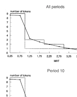
Fig. 1 presents the data for average investments in A for all treatments together, i.e. the aggregate contribution functions. The top portion of the figure corresponds to the data over all periods while the bottom portion shows the results for period 10, the last period.
Fig. 1. Aggregatge contribution functions and step function approximations.
difference in contributions in situations 1 and 2 appears to be quite small. The data exhibit a rather large jump after situation 2, with a steady decline from there on. This smooth pattern stands in contrast to the more erratic behavior of the empirical contribution rates shown by Palfrey and Prisbrey (1996). In their data there are considerable differences in contribution rates for different mrts below 1. For mrts above 1 the contribution rates they observe fluctuate up and down.
first type of step function starts at any number x of tokens and imposes at most one downward step to any number y (,x) of tokens, where x, y, and the location of
9
the step are determined by minimizing the sum of squared errors. This step function will be directly comparable to the one predicted by standard theory. The second type of function allows for multiple steps, with steps at any location and for any number of tokens between 0 and 9 to be allocated at any mrt. The functions that minimize the sum of squared errors for both types are also shown in
10
Fig. 1. We refer to these as the ‘1-step’ and ‘m-step’ function, respectively. Over all individuals, the estimated m-step function which minimizes the sum of squared errors of individual deviations, exhibits more than one step (Fig. 1). The estimated step function for all periods has four steps and the one for period 10 has three steps. Observe that for the first two mrts the value of both m-step functions in Fig. 1 is 9 and for the last two it is 0. According to these estimated functions, in the aggregate, subjects do invest all their tokens in account A, when it is a dominant strategy to do so. In addition, they do not put anything into account A, when it is inefficient to do so. For all periods taken together this contribution function predicts the contribution of 12 out of 54 tokens in situations 3–8, where standard theory predicts 0. The sum of squared errors for this m-step function is 33.07.
Next, consider the general class of 1-step functions. The sum of squared errors is minimized within this class, when x59, y51, with the downward step at mrt51. This yields a sum of 42.01. By comparison, a contribution function with a step from 9 to 2 at mrt51 yields a sum of 42.41, and 9 to 3 gives 51.79.
Finally, consider the contribution function corresponding to standard theory. This is a 1-step function with the step from 9 to 0 tokens, at mrt51. It turns out that this 1-step function is only optimal if we set the restriction y50, i.e. if we directly impose part of the standard prediction on the data. This yields a sum of squared errors of 57.62. Thus, in the general class of 1-step contribution functions, the standard one is outperformed by three other 1-step functions. Moreover, the more general estimated m-step function seems to outperform this restricted 1-step function considerably. Note, however, that we have not corrected for the number of degrees of freedom used. Therefore, it is difficult to draw strict conclusions
11
from this last comparison.
The position of the rational model vis-a-vis alternative models of behavior is weakened considerably by the fact that it is not even the best within the class of
9
The 1-step function with x59 and y50 is the one investigated by Palfrey and Prisbrey (1996). They minimize absolute errors, which gives the same result as minimizing the sum of squared errors in their case.
10
In the present setting, this procedure for the m-step function yields the integer number of tokens closest to the average contribution observed, for any mrt.
11
1-step contribution functions. Over all periods we observe an average percentage of the efficient allocation of 21% (decreasing from 29% in period 1 to 12% in period 10). We cannot straightforwardly test whether this number is significantly
12
different from 0 in a statistical sense, however. However, as will be shown in Section 4, this average behavior is the outcome of the aggregation of very different individual behavior. A sizeable fraction of subjects (just over 40%) exhibit behavior which is best described by an individualistic (i.e. x59, y50) 1-step contribution function. However, there is also a substantial fraction of individuals that purposefully deviates from the individualistic 1-step function. We will show that the average percentage of the efficient allocation for situations 3–8 is
13
significantly different between these two groups.
3.2. Treatment effects on aggregate behavior
As mentioned in Section 2, we investigated the effects of three treatments (homogeneous vs. heterogeneous situations, partial vs. full information and partners vs. strangers) on the percentage of the efficient allocation contributed to the public account in situations 3–8. In aggregate we observe almost no treatment effects, however. Testing for all possible combinations of the three treatments, only the main effect of full vs. partial information was found to be statistically significant (F54.00, P50.05) at the conventional levels. Apparently, at the aggregate level giving better information about the (sum of) contributions of other group members yields higher contributions. This is a first indication that cooperation is affected by what others do. In the next section, we shall show that the effect of information at the aggregate level is the result of distinct effects across groups of individuals: not every (type of) individual is affected to the same
14
extent by the information condition.
The lack of difference in behavior between partners and strangers is not consistent with the original evidence of Andreoni (1988), where strangers contribute more than partners. His result has not always been replicated, however. Keser and van Winden (1997) and Andreoni and Croson (1998) survey the available evidence on this matter. They report that the direction of the effect of the partners–strangers distinction on behavior varies across data sets. In our data we
12
A t-test is not applicable, because we are testing a value at the corner of the choice set.
13
Our evidence can also shed some light on the validity of the notion, suggested by Anderson et al. (1998), that mistakes depend on the costs of making them. In Table 1 one can see that the costs of deviating from the dominant choices are 3 for situations 2 and 3, and 9 for situations 1 and 4. According to this mistakes hypothesis, errors should, therefore, lead to similar deviations for situations 2 and 3, as well as for situations 1 and 4. As can be seen in Fig. 1, our data do not support this notion. Brandts et al. (1999) elaborate on this.
14
find no difference. Our interpretation of this fact is that the forward-looking attribute does not have a significant impact on behavior in our experiments.
3.3. Comparison with results from previous work
When using a new experimental design for an old economic problem, the question whether it yields different behavior than previous designs should be addressed. It turns out that our results are quite similar to those of previous studies. The contribution levels we find are in line with those typically found in the literature. Comparing our results with those in studies with more than one mrt (Isaac et al., 1984; Saijo and Nakamura, 1995; Palfrey and Prisbrey, 1997), the contribution levels in our experiments fall in between the levels found there for similar levels of the mrt. Moreover, as in these studies, we find a decrease in contributions with rising mrt.
Significant decreases of contributions from repetition are reported, among
15
others, by Isaac et al. (1985), Isaac et al. (1994) and Andreoni (1988). This phenomenon is also present in our data. The percentage of the efficient allocation decreases from 29% in period 1 to 12% in period 10. Note that there is still a substantial amount of contributions in period 10. Isaac et al. (1994) provide evidence that suggests that this typical result of lpgg experiments is not simply a decay towards zero contribution that is cut off after 10 rounds. When they extend
16
the number of periods, the rate of decay decreases correspondingly.
Another feature of the existing experimental evidence is that individual subjects tend to split their endowment between the public and the private account (cf. Isaac et al., 1984). Average contribution rates do not reveal this, since they can be the result of some individuals contributing everything and others nothing. Our analysis of individual contribution functions in Section 4 will show that splitting does take place. In particular, a large number of splitting decisions occur between mrt51 and mrt54. Although splitting does decrease towards period 10, it certainly does not go down to 0.
4. Individual results
We now turn to an analysis of behavior across individuals. In this section, we will present evidence from our data that shows that individual behavior is purposeful and diverse and will describe the behavior of different types of subjects. We think that the diversity in behavior may provide a behavioral basis for
15
See, however, Saijo and Nakamura (1995) for a case of no decay.
16
explanations of observed behavior over time in this type of experiment (cf. Section
17
5).
4.1. A classification based on questionnaire responses
If we want to use a classification of individuals to test for differences in choices, we cannot use observed choices for this classification. In our experiments more independent data can be obtained from the post-experimental questionnaire. This included the statement ‘In this experiment, one must try to work together with others, in order to have everyone end up with more money’, with which subjects could disagree or agree on a seven-point scale.
We used responses to this question to classify subjects as individualists (responses 1 or 2, n542), cooperators (6 or 7, n5105) or ‘unclassified’ (3, 4 or
18
5, n542). The average percentage of the efficient allocation is 13.7%, 19.6% and 23.8% for individualists, unclassified and cooperators, respectively. The difference between individualists and cooperators is highly significant (Mann– Whitney, P50.003). These results show that cooperators contribute amounts that are significantly higher than those contributed by individualists, and, hence, different from 0. The observed deviation of aggregate choices as shown in Fig. 1 is, therefore, at least partially due to the purposeful behavior of a substantial number of subjects.
4.2. Analysis of individual contribution functions
Next, we derive a representative step function per individual and use that information to describe behavior. As pointed out above, an important motivation for using the contribution function approach is to obtain more detailed information on individual choices than is possible with other methods. For every individual our design yields one contribution function for each of the 10 periods. We have, therefore, the same information for each of the subjects. Using this information we estimate the step function that minimizes the sum of squared errors over all 10 periods for each individual and classify individuals according to their step function.
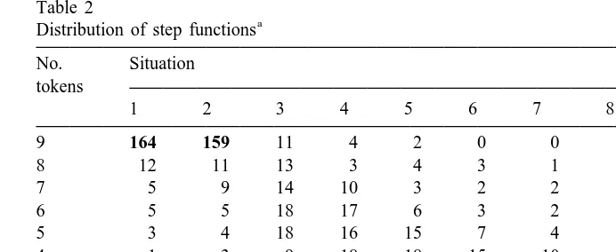
Table 2 presents, for each situation, the distribution of estimated levels of contribution in the step function. This table shows, for example, that the number of individuals who follow a dominant strategy (in their estimated step function) is
17
Offerman et al. (1996) and Suleiman and Rapoport (1992) present evidence that individuals differ consistently with respect to behavior in this type of experiment.
18
Table 2
Each cell gives the number of individuals that had an estimated contribution in their step function at the specified level (row) for the specified situation (column). The number of individuals at the contribution level of the aggregate m-step function (cf. Section 3.1) is given in bold.
85.4%, 82.8%, 78.6% and 83.3% for situations 1, 2, 9 and 10, respectively, i.e. for the situations where this dominant strategy yields efficiency. For the situations where the dominant strategy is not efficient, one mode of the distribution is always at this strategy, but the percentage of individuals following it varies from 28.1% to 62.0%.
We can allocate individuals into different groups, according to the characteris-tics of their step function. We do this for all periods combined as well as for period 10. First, consider the subjects who invest all their tokens in account A when it is a dominant strategy to do so, do not invest any tokens in A when it is inefficient to do so, and do not have any upward steps in their step function. Out of a total of 192, the estimated step function of 139 subjects (72.4%) exhibited this type of behavior. This group of subjects is easiest to categorize, because their estimated step functions are on the one hand consistent with rational theory whenever this does not conflict with efficiency and on the other hand show a consistency across mrts that is in line with intuition. In what follows, we only consider this group, leaving 53 subjects (27.6%) unclassified. These subjects can be categorized using more ad hoc rules. Our conclusions are robust to such extensions.
Out of these 139 subjects, 51 have step functions with only one step going from 9 to 0 and, out of these 51, 50 have the step between situations 2 and 3. These 50 individuals are estimated to behave strictly according to the game-theoretic prediction and we will call them clear individualists. The remaining subject with a 1-step function has a cutoff point between situations 3 and 4. We will interpret this as a kind of cooperative behavior.
multiple-step function presented in Section 3 is the result of a substantial fraction of subjects using multiple-step functions. Of these 88 subjects, 28 exhibit a step function with just 6 tokens or fewer for situations 3–8 (a percentage of the efficient allocation of 11% or less). We will call these subjects semi-individualists
19
and the remaining 60 subjects cooperators.
As a whole, the categorization implies that we estimate the share of in-dividualists (including semi-inin-dividualists) and cooperators to be 40.6% and 31.8%, respectively, and leave 27.6% uncategorized. These shares are consistent with the number of individualists and cooperators typically found (cf. Offerman et al., 1996).
One can make the same classification using decisions in period 10 only. In that case, 66.7% of our subjects are classified as individualists (including semi-individualists) and 25.0% as cooperators or altruists, while 8% remain unclassified. Hence, classifying on the basis of period 10 means a relative increase in individualists compared to a classification on the basis of all periods.
5. What kind of ‘other-regarding’ preferences can accommodate our data?
We have found that aggregate behavior in our data deviates from the one corresponding to own payoff maximization, and that a large fraction of subjects deviates from it intentionally, motivated by some kind of other-regarding preferences. In this section, we attempt to shed some light on the characteristics of these non-selfish preferences.
A central distinction between different formulations of other-regarding prefer-ences is whether subjects’ contributions in a lpgg are sensitive to the contributions of other participants. Linear altruism and a simple warm glow formulation predict that subjects’ behavior is independent of that of others. We now present some evidence from our experiments that cannot be accommodated by formulations of
20
this type.
First, the development of aggregate behavior over time in the partners sessions shows that contributions tend to become concentrated in specific groups in later periods. We measure the concentration by considering two inequality indices, the Theil (1967) coefficient and the Gini coefficient (the area between the Lorenz curve and the 458 line). The data show a small increase in inequality between periods 1 and 10 for the strangers sessions and a larger increase for the partners
19
The number of 6 tokens is chosen fairly ad hoc. We are mainly interested in comparing the categorizations overall and in period 10, however. Our conclusions from this comparison are robust to the cutoff point chosen to distinguish semi-individualists from cooperators.
20
sessions. The statistical properties of these coefficients are not known, and exact values are difficult to interpret. Therefore, we used a bootstrap method to determine how likely it was to find the inequality we observe. To see how this was done, consider all 96 individual contributions (24 groups of four) in period 1 of the partners sessions. In 10 000 iterations we randomly allocated these individual contributions to 24 groups of four. This gives 10 000 Theil and Gini coefficients. We ordered these 10 000 values (once each, for both coefficients) and determined how many values were larger than the one we observed. We followed the same process for partners in period 10 and for strangers in periods 1 and 10.
The result of this bootstrap is that the concentration of contributions in groups (as measured by both inequality indices) measured in the strangers sessions in period 10 are not significant at the conventional levels. The same holds for both coefficients in period 1 of the partners sessions. The inequality measured by the two coefficients for period 10 of the partners sessions is very unlikely to be randomly determined, however. Only 0.3 of the Gini coefficients generated by our bootstrap were higher and 0.2 of the Theil coefficients. Hence in the partners sessions we observe a concentration of contributions in specific groups in period 10.
Second, consider the classification based on the actual choices over all periods and over period 10 presented in Section 4.2. A comparison of average earnings in all periods between the 50 individualists and the 61 cooperators reveals that individualists earn more (fl. 38.40 vs. fl. 36.29; Mann–Whitney, P50.003). On the other hand, a comparison of average earnings between those subjects which we feel we can confidently classify either as individualists or as cooperators in period 10 shows that the latter earn more in this period (fl. 3.61 vs. fl. 3.71), although the difference is not statistically significant (Mann–Whitney, P50.55). The fact that they are earning more in this linear setting is another indication that cooperators are concentrated in groups in period 10.
strangers do. These effects seem to imply that more contributions are observed by cooperators when it is easier to find out whether or not other cooperators are present in the group. The effect of partial vs. full information is strong enough to show up at the aggregate level in Section 3.2. In conclusion, this analysis of treatment effects provides more evidence that (some) subjects’ behavior is
21
influenced by that of other participants.
All in all, we believe that there is a considerable amount of evidence that points to subjects’ behavior being interdependent. Our results do not allow us to characterize more completely the motivational basis for this interdependence, however. At this point, different explanations of interdependent behavior could be consistent with the data.
A form of cooperation that is consistent with all of our findings can be found in the classical psychological literature on differences in individual ‘value orienta-tion’ and the way in which different types of individuals interact over time (e.g. Kelley and Stahelsky, 1970). For a review, see Offerman et al. (1996), where an application to experimental economics is given. An important element in this literature is that there are significant differences across subjects in motivation. In short, this theory would predict for our experiments that there is a substantial number of individuals who try to tacitly cooperate. However, these individuals switch to individualistic behavior if confronted with too many non-contributors.
We conjecture that the interaction between the two types we distinguished (cooperators and individualists) provides an explanation of changes in behavior over time. In the post-experimental questionnaire, various subjects described their motivation in a way that is much like this notion. When asked to motivate their decisions, many subjects referred to notions like ‘working together to earn more’ and various people noted that up to situation 8, everyone could be better off if they coordinated actions. For example, one subject stated: ‘‘Every time, I calculated what the revenue from A would be if all chose A. It seemed to make sense that everyone in situation 3, for example, would put a lot in A (4312548415), but this did not happen. [ . . . ] When I observed that other people put less in A than I did, I subsequently saw less advantage to putting money in A’’. In Brandts and
21
Schram (1996) we develop this interaction between the two types of individuals formally, using a notion that we call ‘cooperative gain seeking’.
6. Summary and conclusions
One of the advantages of experiments in economics is that they often can be designed in ways that allow the observers to obtain very rich data. The contribution function design for lpgg experiments that we present in this paper is a very efficient way of generating a large set of data about complete individual decision rules, permitting a more detailed analysis of individual behavior than previous designs do.
We find that aggregate behavior can be characterized by a multiple-step function, both for average behavior over time and for behavior in the last experimental period. For average behavior over time the percentage of the efficient allocation to the public account for the relevant set of situations is 21%, while for the last period it is 12%. Aggregate behavior in our experiments, therefore, does not seem consistent with the dominant strategy Nash equilibrium prediction even though a substantial fraction of subjects does follow this prediction.
The question is, whether the use of multiple steps can be interpreted as errors or as some kind of purposeful behavior. In our view there are several reasons why noise cannot be a full explanation of our data. First, we find a strong positive relation between subjects’ intention to contribute and a broad-based measure of contributions. Second, our data for average behavior only deviates substantially from the theoretical prediction for those situations where tacit cooperation can lead to efficiency gains and hence, those cooperating can become better off. In other words, we do not find symmetry of the deviation from the standard prediction around mrt51. For instance, for mrt50.75 we find all tokens invested to be the best estimation of individual behavior, while not 0 but 3 tokens is the best estimation of behavior for mrt51.25. Third, the fact that a large fraction of individuals consistently (over 10 periods) contributes substantial amounts is further evidence against the error hypothesis. In an errors interpretation one would expect
22
these individuals to sometimes contribute much, sometimes little.
Our design facilitates the identification of diversity of behavior across subjects: we find that a substantial fraction of subjects behave in the way predicted by standard theory, while another sizeable group deviates substantially from that behavior.
In our view, the question to be addressed is no longer whether cooperation takes place, but what kind of cooperative model will best explain the data from lpgg
22
experiments. Palfrey and Prisbrey (1997) attribute observed contributions to a combination of warm glow and error. Our analysis in Section 5 casts some doubt on warm glow and linear altruism being the only kind of other-regarding behavior, however. We show that the concentration of contributions increases over time in the partners condition. Our data also show that in period 10 cooperators earn more than individualists. The differential impact of some of the treatments on subjects with different motivations is a final indication that more than a simple warm glow plus linear altruism model is needed to explain the data.
We believe that our results add more strength to the evidence from previous research that shows that in small groups subjects are able to obtain gains from cooperation, even in the absence of ‘proper’ incentives. As discussed in some detail in Hoffman et al. (1995), the basis for this ability to cooperate may perhaps be found in the evolutionary fitness of certain cognitive abilities which predispose people towards this kind of behavior.
Acknowledgements
The authors would like to thank Joep Sonnemans for useful comments and his help in conducting the experiments, Tanga McDaniel, Mark Olson and two anonymous referees for helpful comments, and Otto Perdeck for his programming. We are grateful to Ingrid Seinen for valuable research assistance. The participants at the 4th Amsterdam Workshop on Experimental Economics (AWEE95), the 1995 ESA conference in Tucson, and the 1996 North American Public Choice Society / ESA Conference in Houston presented useful remarks on a previous version of this paper. The authors acknowledge financial support from the Dutch NWO (PGS 45-96) and the Spanish DGCICYT (PB 92-0593, PB 93-0679 and PB 94-0663-C03-01). This paper is part of the EU-TMR Research Network ENDEAR (FMRX-CT98-0238).
Appendix A
INTRODUCTION
You are about to participate in an experiment about decision-making. The money for this study has been provided by various institutions. The
instructions are simple and if you follow them carefully, you will be able to earn a considerable amount of money. All the money you earn during
this experiment will be yours to keep. It will be paid to you personally in cash at the end of today’s session. In addition to the money you will
earn, you have already received a show-up fee of 500 pesetas [5 guilder] when you came in.
Now press F2 to continue.
INTRODUCTION
Please take your time to read these instructions at your own pace. If you have any questions while reading them, please raise your hand and
someone will come to your table. Before the experiment, two practice rounds will be played, which will not be paid.
Throughout these instructions, you may return to a previous page by pressing F1 and proceed to the next page by pressing F2.
F15previous F25next
PERIODS AND GROUPS
The experiment consists of 10 separate periods. In each period, you are in a group with three other participants. The other participants in your
group remain the same in all 10 periods. You will not know which of the other participants is in your group. The group composition is secret for
every participant.
In each period, you and the other participants in your group have to make decisions. The amount of money you earn depends on your own
decisions and on the decisions of the three other members in your group.
The monitor has a separate role. This will be explained later in the instructions.
DECISIONS: TOKENS
In each period of the experiment, you will have 9 tokens. You must invest each token either in ACCOUNT A or in ACCOUNT B. The amount of
money you earn depends on your division of the tokens, on the division by other group members and on chance.
F15previous F25next
DECISIONS: ACCOUNT A
Each token you invest in account A yields 8 pesetas [12 cents] to YOU as well as to EACH MEMBER OF YOUR GROUP. You (and everyone
else in your group) also receive 8 pesetas [12 cents] for each token invested in account A by other group members.
F15previous F25next
DECISIONS: ACCOUNT B
Your investment in account B yields money for YOU ALONE. Other group members do not receive anything for your investment in account B.
The amount of money you receive per token invested in account B differs per ‘situation’. There are 10 different situations that may occur. Which
situation holds for you will be determined by chance. This is explained below.
F15previous F25next
DECISIONS: 10 SITUATIONS
The amount of money you earn per token in account B is different for each of the 10 situations. We call this amount the B-VALUE for the
situation. Note that the amount related to account A is always 8 pesetas [12 cents] per token.
At the beginning of each period you will have to tell us how you want to divide your tokens between the two accounts for each of the 10
situations.
YOUR DECISIONS ON THE COMPUTER
SCREEN [1]
To report your decisions, you will be able to use a decision screen like this one. Note that the 10 situations are represented by rows on the screen.
F15previous F25next
INFORMATION ON THE SCREEN
SCREEN [1]
The first two columns (on the left half of your screen) show the payoff per token in accounts A and B. The amount is 8 pesetas [12 cents] PER
GROUPMEMBER for every token invested in A.
In Situation 1, the payoff (B-value) is 2 pesetas [3 cents] FOR YOU ALONE for every token you invest in B.
For Situation 2 the B-value is 6 pesetas [9 cents], etc.
F15previous F25next
INFORMATION ON THE SCREEN
SCREEN [1]
For Situation 10, the B-value is 38 pesetas [57 cents].
These numbers will be given on your screen, handed out on paper, and projected on the overhead-screen.
F15previous F25next
DECIDING FOR A SITUATION
SCREEN [2]
to enter your decision. If you want to change your decision, you may always re-choose the situation concerned later.
Now choose a situation and press ENTER.
Then you may continue with the instructions by pressing F2.
ARROWS: choose; press ENTER.
DIVIDING YOUR TOKENS
When you are going to enter your decision for a situation, you will be asked to divide 9 tokens over A and B.
Shortly, you will be given the opportunity to practice giving a division of the tokens. First we will go through the various steps.
F152 pages back F25next
DIVIDING YOUR TOKENS
First you choose A or B using the ARROW keys. Then you type the number of tokens you wish to invest in that account. When you are finished,
press ENTER. The computer will automatically invest the rest of your tokens in the other account. If you want to change your choice, simply
choose A or B and enter a new number.
F15previous F25next
DIVIDING YOUR TOKENS
Press ENTER again to enter your choice for this situation. Remember that you may return to this situation to change your decision later.
On the next screen you may practice dividing your tokens for situation 2. This is just to practice using the screen, your choice will not be
registered or used in any way.
DIVIDING YOUR TOKENS
SCREEN [3]
Now try entering an investment decision. First choose A or B (using the arrows). Enter a number between 0 and 9. Press ENTER. Confirm by
pressing ENTER again.
F15previous F25next
YOUR CHOICE APPEARS ON THE SCREEN
SCREEN [4]
Note that your choice is given in yellow on the right half of your screen. In parentheses, we multiply your investment in tokens with the amount
per token, as given on the left half of your screen. We only do this to help you with your calculations.
The amount in parentheses is not equal to your total earnings, for two reasons. First of all, you also earn money from investments in account A by
other group members. Second, only one situation is actually played. How this is done will be explained shortly.
F15dividing your tokens F25next
CONFIRMING YOUR CHOICES
After you are satisfied with your decision for all situations, you must confirm your choices by pressing F10. You will be asked to finalize these
decisions. After that, it is no longer possible to change your decisions for that period.
You may have to wait a little while for other participants to finish deciding. When everybody has finalized their decisions, we will come by and
select the situation that will be played. We will now explain how this is done.
F15previous F25next
A SITUATION IS SELECTED
be chosen. This is done separately and privately for each
participant. Generally, different B-values will be chosen for the various group members.
We will come to your table and throw a 10-sided die (with sides ‘0’ through ‘9’). The result determines the situation chosen for you, where a ‘0’ is
interpreted as ‘10’.
You are not permitted to tell anyone about your decisions or the situation selected for you. We will enter the situation selected in your computer
to allow the central computer to determine the outcome for the period.
F15previous F25next
YOUR EARNINGS FOR THE PERIOD FROM ACCOUNT A
For each participant the separate throw of the die will determine which of the divisions of tokens will be used to calculate earnings. You will see
that the situation selected will be highlighted on your screen. The situations selected for various participants determine the ACTUAL amounts of
tokens invested in accounts A and B by each of the participants.
The computer will use this information first to determine the total number of tokens invested in A by members of your group. Multiply this
number by 8 pesetas [12 cents] to determine your earnings from account A.
F15previous F25next
YOUR EARNINGS FOR THE PERIOD FROM ACCOUNT B
Your earnings from account B are determined by considering the situation selected for you (with a corresponding B-VALUE) and the number of
tokens you invested in B for that situation. Multiplying your investment by the B-VALUE gives your earnings from account B.
Your total earnings in a period are equal to your earnings from account A PLUS your earnings from account B.
THE REGISTRATION WINDOW
SCREEN [5]
The computer will do all calculations and registration for you. On the left half of your screen you may see how the latter is done. At all time in
the experiment, you may choose to have this information on your screen.
If you press the key ‘F1’ later, the information will alternatively appear in a small (only a few periods), large (all previous periods) or no window.
You cannot try this now. Later in the practice rounds you may try the options concerning the presentation of the registration.
F15previous F25next
CALCULATIONS AND REGISTRATION
SCREEN [5]
Consider the information given in the registration window. For each period, you first see the period number and the situation selected for you in
that period.
Next the table shows your division of 9 tokens for that situation.
The fifth column gives the total number of tokens invested in A by members of your group.
The last column gives your earnings for that period. The computer determines this by multiplying the number in column 5 by 8 and adding the
earnings from B. The earnings from B are determined by your investment (column 4) and the B-VALUE in the situation of column 2. Your total
earnings to date are given at the right bottom corner of the registration table and later on the top right corner of your screen. If you have any
questions about your earnings at any time, please raise your hand.
F15previous F25next
NEXT PERIOD
After the earnings have been calculated and registered for everyone, we will proceed to the next period.
This will continue for 10 periods.
RECALLING PREVIOUS CHOICES
When making your decisions, you may want to recall your choices from the previous round. By pressing F2, you will see these previous choices
on a window like the one on the right. The numbers in the window now have no particular meaning. We just want to show you what the window
looks like.
While this window is on your screen, you cannot enter choices. You must first press F2 again to cancel the window. Then you can enter your
choices.
You may try this later, in practice round 2, by recalling your choices from practice round 1.
F15previous F25next
PAYMENT
At the end of today’s session we will pay you in cash the amount of money that you will have earned in 10 periods. In addition, you have already
received 500 pesetas [5 guilder] cash for your participation. Your earnings are private information. You do not need to tell them to anyone.
We stress again, that you are not allowed to talk or communicate with other participants. If you have a question, just raise your hand. We will
come to your table.
F15previous F25next
MONITOR
The monitor has two tasks. First of all, (s)he will help us with the random selection of a situation. We will explain how this is done when it is
time to select a situation.
Besides this, the monitor may check that everything is taking place as described in the instructions. To help her or him with this, we will give the
monitor an overview of the group composition at the beginning of the experiment. With this, (s)he may check whether the reported investment in
The monitor is not allowed to talk or communicate directly with other participants. If the monitor believes that something is not taking place in
accordance with the instructions (s)he must report to the experimenter.
The monitor’s earnings do not depend on the decisions made today. (S)he will receive the average payment of the previous experiment.
F15previous F25next
PRACTICE ROUNDS
When everyone has finished with the instructions, we will play two practice rounds. In these practice rounds, you will not be playing in groups.
The computer will make up decisions for other members randomly. Therefore, the practice rounds cannot give you information about what you
may expect from other participants. These practice rounds will not be paid.
F15previous F25next
RE-READ
This brings you to the end of the instructions. If you would like to reread something, you may choose one of the keys F1–F9. Choose F2 to
indicate that you are finished with the instructions. With F10 you will return to this menu.
F15previous page
F25FINISHED WITH THE INSTRUCTIONS F35Introduction
F45Instructions about accounts A and B F55Instructions about reporting decisions
F65Instructions about selecting a situation and determining your earnings F75Instructions about the registration of the results
F85Instructions about recalling previous decisions F95Instructions about the monitor
choose from: F1 F2 F3 F4 F5 F6 F7 F8 F9
FINISHED
You may still reread parts of the instructions. When everyone has indicated that they are finished, we shall stop the instructions and start the
practice rounds, however.
PLEASE WAIT QUIETLY UNTIL EVERYONE IS FINISHED WITH THE INSTRUCTIONS
choose from: F1 F2 F3 F4 F5 F6 F7 F8 F9
References
Anderson, S.P., Goeree, J.K., Holt, C.A., 1998. A theoretical analysis of altruism and decision error in public goods games. Journal of Public Economics 70, 297–323.
Andreoni, J., 1988. Why free ride? Strategies and learning in public goods experiments. Journal of Public Economics 37, 291–304.
Andreoni, J., 1990. Impure altruism and donations to public goods: A theory of warm-glow giving. Economic Journal 100, 464–477.
Andreoni, J., 1995. Cooperation in public-goods experiments: Kindness or confusion? American Economic Review 892, 891–904.
Andreoni, J., Croson, R., 1998. Partners versus strangers: Random rematching in public goods experiments, Mimeo, University of Wisconsin.
Bolton, G.E., Brandts, J., Katok, E., 2000. How strategy sensitive are contributions? A test of six hypotheses in a two-person dilemma game. Economic Theory, in press.
Bolton, G.E., Ockenfels, A., 2000. ERC: A theory of equity, reciprocity and competition. American Economic Review, in press.
Brandts, J., Saijo, Y., Schram A., 1999. A four country comparison of spite, cooperation and errors in voluntary contribution mechanisms, Mimeo, University of Amsterdam.
Brandts, J., Schram, A., 1996. Cooperative gains or noise in public goods experiments, Tinbergen Institute Discussion Paper 96-81 / 1, University of Amsterdam.
Fehr, E., Kirchsteiger, G., Riedl, A., 1993. Does fairness prevent market clearing? An experimental investigation. The Quarterly Journal of Economics 108, 437–460.
Fehr, E., Schmidt, K., 1999. A theory of fairness, competition and cooperation. Quarterly Journal of Economics CXIV, 817–868.
Fisher, J., Isaac, R.M., Schatzberg, J., Walker, J., 1995. Heterogeneous demand for public goods: Behavior in the voluntary contributions mechanism. Public Choice 85, 249–266.
Hoffman, E., McCabe, K., Smith, V., 1995. Behavioral foundations of reciprocity: Experimental economics and evolutionary psychology, Mimeo, University of Arizona.
Isaac, R.M., McCue, K., Plott, C., 1985. Public goods provision in an experimental environment. Journal of Public Economics 26, 51–74.
Isaac, R.M., Walker, J., Thomas, S., 1984. Divergent evidence on free riding: An experimental examination of possible explanations. Public Choice 43 (1), 113–149.
Isaac, R.M., Walker, J., Williams, A., 1994. Group size and the voluntary provision of public goods: Experimental evidence utilizing large groups. Journal of Public Economics 54, 1–36.
Kelley, H.H., Stahelsky, A.J., 1970. Social interaction basis of cooperators’ and competitors’ beliefs about others. Journal of Personality and Social Psychology 16, 66–91.
Keser, C., van Winden, F., 1997. Partners contribute more to public goods than strangers, Tinbergen Institute Discussion Paper 97-018 / 1, University of Amsterdam.
Ledyard, J., 1995. Public goods: A survey of experimental research. In: Kagel, J., Roth, A. (Eds.), The Handbook of Experimental Economics. Princeton University Press, pp. 111–194.
Levine, D.K., 1998. Modeling altruism and spitefulness in experiments. Review of Economic Dynamics 1 (3), 593–622.
Offerman, T., Sonnemans, J., Schram, A., 1996. Value orientations, expectations, and voluntary contributions in public goods. Economic Journal 106, 817–845.
Palfrey, T.R., Prisbrey, J.E., 1996. Altruism, reputation and noise in linear public goods experiments. Journal of Public Economics 61, 409–427.
Palfrey, T.R., Prisbrey, J.E., 1997. Anomalous behavior in public goods experiments: How much and why? American Economic Review 87, 829–846.
Rabin, M., 1993. Incorporating fairness into game theory and economics. American Economic Review 83, 1281–1302.
Sefton, M., Steinberg, R., 1996. Reward structures in public good experiments. Journal of Public Economics 61, 263–287.
Saijo, T., Nakamura, H., 1995. The ‘spite’ dilemma in voluntary contribution mechanism experiments. Journal of Conflict Resolution 39, 535–560.
Suleiman, R., Rapoport, A., 1992. Provision of step-level public goods with continuous contribution. Journal of Behavioral Decision Making 5, 133–153.