The Long- Run Effects of Large- Scale
Physical Destruction and Warfare on Children
Mevlude Akbulut- Yuksel
Akbulut- YukselA B S T R A C T
This paper provides causal evidence on the long- term consequences of large- scale physical destruction on educational attainment, health status, and labor market outcomes of children. I exploit the plausibly exogenous region- by- cohort variation in the intensity of World War Two (WWII) destruction as a unique quasi- experiment. I fi nd that exposure to destruction had long- lasting detrimental effects on the human capital formation, health, and labor market outcomes of Germans who were at school- age during WWII. An important channel for the effect of destruction on educational attainment is the destruction of schools whereas malnutrition is partly behind the estimated impact on health.
I. Introduction
Armed confl icts have become more common and more physically
destructive in recent years (Collier, Hoeffl er, and Rocher 2009). Almost one- third
of the countries around the globe have experienced civil war and violence during the
fi rst decade of the 21st century (Minoiu and Shemyakina 2012). Large and aggregate
Mevlude Akbulut- Yuksel is an assistant professor of economics at Dalhousie University and a Research Fellow in IZA and HICN. She is grateful to Randall Akee, Richard Akresh, Joshua Angrist, Aimee Chin, Barry Chiswick, Deborah Cobb- Clark, Damien de Walque, Nicola Fuchs- Schundeln, Daniel Hamermesh, Tarek Hassan, Scott Imberman, David Jaeger, Chinhui Juhn, Melanie Khamis, Ben Kriechel, Adriana Kugler, Lars Osberg, David Papell, Shelley Phipps, Daniel Rosenblum, Olga Shemyakina, Belgi Turan, Ge-rard van den Berg, Courtney Ward, and Mutlu Yuksel as well as seminar participants at Georgia Institute of Technology, Dalhousie University, Oxford University, University of Alicante, University of Texas Pan American, DIW Berlin, and IZA; 2009 IZA/CEPR European Labor Symposium; 2009 SOLE; 2008 HICN’s Annual Workshop; 2008 NEUDC; 2008 IZA/World Bank Conference; 2008 European Summer School in Labor Economics and University of Houston Workshop for their helpful comments and suggestions. She is also grateful to Stephen Redding and Daniel Sturm for kindly providing her with their refugee data. She thanks IZA for providing fi nancial support and a stimulating research environment. She is responsible for any errors that may remain. The data used in this paper are proprietary. Historical data are available through German public libraries. Researchers may apply for use of the GSOEP data through DIW Berlin. The author is willing to advise on this process.
[Submitted April 2011; accepted August 2013]
ISSN 0022- 166X E- ISSN 1548- 8004 © 2014 by the Board of Regents of the University of Wisconsin System
shocks caused by armed confl icts have devastating consequences for a country includ-ing loss of lives, displacement of people, destruction of physical capital and public in-frastructure, and reduced economic growth. Evidence from macro- level studies shows
that countries experience rapid recovery after wars and armed confl icts and return to
their steady state within 20–25 years (Miguel and Roland 2011; Brakman, Garretsen, and Schramm 2004; Davis and Weinstein 2002). However, a growing literature on
the micro- levels effects of armed confl icts fi nds that armed confl icts infl ict direct and
external costs on survivors that last longer and can be as detrimental as the physical
impacts.1 Among survivors, children are especially adversely affected by the armed
confl icts given the age- specifi c aspect of human capital investments.
This paper provides causal evidence on long- term consequences of wars and armed
confl icts on the educational attainment, future health, and labor market outcomes of
children. Specifi cally, I explore region- by- cohort variation in destruction in
Ger-many arising from the Allied Air Forces (AAF) bombing throughout World War Two (WWII) as a unique quasi- experiment. During WWII, more than 1.5 million tons of bombs were dropped in AAF aerial raids on German soil, destroying about 40 percent of the nationwide total housing stock (Diefendorf 1993). Because WWII was a major, transformative event in modern history, it is important to understand its long- term household- level effects. Moreover, civil wars pose substantial threats to the well- being
of millions of children around the globe today (Collier, Hoeffl er, and Rocher 2009).
Therefore, it is policy- relevant to analyze the long- run micro- level effects of armed
confl icts and the mechanisms through which they affect children to devise policies and
programs to stem and reverse these effects.
This study is related to the broader literature exploring the association between wars and macroeconomic indicators. Studies that examine the long- run effects of U.S. bombing during WWII in Japan (Davis and Weinstein 2002) and in Germany
(Brak-man, Garretsen, and Schramm 2004) fi nd no evidence for the persistent impacts of the
bombing on city size. Miguel and Roland (2011) revisit the same question using the extensive U.S. bombing campaigns in Vietnam during the Vietnam War. They provide similar evidence suggesting that the U.S. bombing did not have any long- lasting ef-fects neither on physical infrastructure and local population nor on literacy and pov-erty levels, 25 years after the Vietnam War. In contrast to these macro- level studies,
I fi nd that the extensive AAF bombing campaign during WWII has had long- lasting
effects on German children’s human capital formation, future health, and labor market outcomes even four decades after WWII.
This study also contributes to a growing literature examining the immediate and
the long- term effects of armed confl icts on human capital formation. Shemyakina
(2011) fi nds that adolescent girls exposed to civil confl ict in Tajikistan are less likely
to complete secondary school. Leon (2012) and Akresh and de Walque (2008) provide
similar evidence from the armed confl icts experienced in Peru and Rwanda,
respec-tively. In addition, Angrist and Kugler (2008) fi nd that an increase in coca prices and
cultivation escalated the confl ict activities in Colombia and decreased teenage boys’
school enrollment. Similarly, Ichino and Winter- Ebmer (2004) show that Austrian and German individuals who were ten years old during WWII acquired less education; as
a consequence they earned signifi cantly less in adulthood than other cohorts in their countries as well as individuals of the same cohort born in Switzerland and Sweden.
This paper adds to this literature by quantifying the long- term consequences of WWII destruction on educational attainment, height, health satisfaction, adult mortal-ity, and labor market outcomes. I utilize a detailed regional data set on WWII physi-cal destruction in former West Germany from Kaestner (1949) and combine it with
individual- level data from the German Socio- Economic Panel (GSOEP).2 The
rich-ness of destruction data enables me to quantify the realized wartime destruction and explore a detailed spatial variation in wartime destruction intensity within West Ger-many to estimate the long- term effects of WWII on children’s outcomes. In contrast, other studies use a measure of exposure to war that has limited spatial variation (only across countries or across few regions within a country) and they have limited or no in-formation on the intensity of exposure to war (Ichino and Winter- Ebmer 2004; Akresh and de Walque 2008; Shemyakina 2011). In addition, I have also compiled novel data on the number of schools and teachers, postwar education, and health expenditure. Together with a wide range of war- related questions in GSOEP, these data enable me
to rigorously investigate the heterogeneity in the long- term effects of armed confl icts
and formally test potential mechanisms by which armed confl icts affect children’s
outcomes, including parental background, loss of a parent during the war years, de-ployment of a father for war combat, destruction of schools, and absence of teachers. Finally, in contrast to other studies, in addition to difference- in- differences analyses, I employ an instrumental- variable strategy in this paper where distance to London serves as an instrument for the wartime destruction experienced in each region.
This study also is related closely to literature examining the relationship between
armed confl icts and individuals’ health outcomes. Several studies fi nd that children
who were in utero and in their early childhood years during armed confl icts have lower
birth weight and lower height- for- age in their teenage years (Mansour and Rees 2012; Akresh, Lucchetti, and Thirumurthy 2012; Minoiu and Shemyakina 2012; Bunder-voet, Verwimp, and Akresh 2009; Alderman, Hoddinott, and Kinsey 2004). This
pa-per considers longer- run outcomes than other studies; the confl icts studied in other
papers are more recent so very long- run outcomes are yet to be realized. Therefore, to
my knowledge, this is the fi rst paper that provides causal evidence on the long- term
impacts of childhood exposure to warfare and armed confl icts on individuals’ adult
height, self- rated health satisfaction, and mortality.
I employ a difference- in- differences strategy in my analysis that exploits within- region cross- cohort variation in exposure to WWII destruction. The “treatment” vari-able in difference- in- differences estimation is an interaction between regional intensity of WWII destruction and a dummy variable for being school- aged during WWII. The validity of difference- in- differences estimation relies on the presence of parallel trends in schooling, health, and labor market outcomes between the affected, and the control cohorts in regions with varying intensity of wartime destruction. I apply the same difference- in- differences strategy using a sample of individuals who were already
beyond school age when WWII began, and fi nd no evidence of differential trends.
In addition to the difference- in- differences analysis, I use an alternative estimation
strategy and instrument the regional war destruction with region’s distance to London
where AAF airfi elds were mainly located. Due to their proximity to the United
King-dom, areas in the northern and western parts of Germany suffered the most from the AAF aerial bombing during WWII. Distance from London, however, could capture a wide range of factors including economic advantage and might affect children’s long- term outcomes through channels other than WWII destruction. I assess the validity of instrument in Section V by comparing regional prewar characteristics and postwar
education and health expenditure by distance to London and fi nd no variation across
regions.
I fi nd that large- scale physical destruction had detrimental effects on education,
health, and labor market outcomes even after 40 years. First, children who grew up in a region with average WWII destruction have 0.3 fewer years of schooling on aver-age in adulthood with those in the most affected cities completing 0.8 fewer years. Second, these children are more than a half inch shorter in adulthood. Third, children from disadvantaged families have four percentage points higher mortality later in life
and are, on average, six percentage points less likely to be satisfi ed with their health
in adulthood due to wartime destruction. Finally, exposure to war reduces future labor
market earnings of males from disadvantaged families by 9 percent. I also fi nd that the
destruction of schools has long- lasting detrimental effects on the human capital for-mation of German children. Moreover, given the sizable impact on height, it is likely that malnutrition during the war years is an important mechanism for the estimated long- term health effects of WWII.
The remainder of the paper is organized as follows. Section II provides a brief
back-ground of AAF bombing in Germany during WWII. Section III discusses the identifi
-cation strategy. Section IV describes the regional destruction data and individual- level survey data used in the analysis. Section V presents the main results, extensions and robustness checks. Section VI concludes.
II. Background on Allied Bombing of Germany
during WWII
During WWII, Germany experienced widespread bombardment by the AAF. More than 1.5 million tons of bombs were dropped in aerial raids on German soil, destroying or heavily damaging 40 percent of the total housing stock nationwide (Diefendorf 1993). Although most of the destroyed buildings were residential
build-ings, schools, hospitals, and other kinds of public buildings were also demolished.An
overwhelming majority of the AAF’s aerial attacks consisted of night time “area bomb-ing” rather than “precision bombing.” Sir Arthur Harris, the Commander- in- Chief of the Royal Air Force (RAF), regarded area bombing as the most promising method of
aerial attacks. The aim of area bombing was to start a fi re in the center of the each
town, which would consume the whole town. At the same time, Sir Harris and his staff
had a strong faith in the morale effects of bombing and thought Germany’s will to fi ght
could be destroyed by the destruction of German towns (USSBS 1945).
varied substantially. The targeted areas were selected not only because they were particularly important for the war effort but also for their visibility from the air, de-pending, for example, on weather conditions or visibility of outstanding landmarks such as cathedrals (Knopp 2001; Friedrich 2002). Furthermore, regions in northern and western Germany suffered the most destruction because they were easily reached
from English air fi elds. Berlin, for example, was nearly twice as far away from British
airfi elds as the cities in the Ruhr Area, and therefore was not hit as hard until the end
of 1943 (Diefendorf 1993; Grayling 2006).
The foregoing discussion on the historical accounts of the attacks on German soil
suggest that the degree of WWII destruction depended on fi xed regional characteristics
(for example, areas that were larger, closer to England, and had more visible land-marks were more likely to be targets of air raids) and chance (due to technology and weather, the intended exact target was hit and the maximal damage caused only part of the time). In my main analysis, I will take the cross- region variation in intensity of WWII destruction as exogenous to children’s long- term outcomes once I control for
fi xed regional characteristics.
III. Identi
fi
cation Strategy
In this section, I describe my strategy for identifying the causal effect of WWII destruction on education, health, and labor market outcomes of German chil-dren. This strategy exploits the plausibly exogenous region- by- cohort variation in de-struction intensity. This is a difference- in- differences- type strategy where the “treat-ment” variable is an interaction between regional intensity of WWII destruction and a
dummy for being school- aged during WWII.3 In particular, the proposed estimate of
the average treatment effect is given by β in the following baseline region and year of
birth fi xed effects equation:
(1) Yirt= α + β(Destructionr × WWII_Cohortit) + δr+ γt+ π’X irt+ εirt
where Yirtis the outcome of interest for individual i,in region r, born in year t.
De-structionris the measure of war damage in the region r. WWII_Cohortit is a dummy
variable that takes a value of 1 if individual i was at school- age during WWII and zero
otherwise.4δ
ris region- specifi c fi xed effects, controlling for the fact that regions may
be systematically different from each other. γt is the year of birth fi xed effects,
control-ling for the likely secular changes across cohorts. Xirt is a vector of individual
char-acteristics including gender and rural dummies as well as family background and re-gional characteristics, such as parental education and the interaction of prewar rere-gional
population density with birth- year dummies. εirt is a random, idiosyncratic error term.
The standard errors are clustered by region and birth year to account for correlations
in outcomes between individuals in the same region over time.5
Individuals who were born between 1922 and 1939 form the affected cohorts be-cause they were of primary school and upper secondary school age during the war years. Thus, their schooling has the potential to be affected by exposure to WWII
destruction.6 On the other hand, individuals born between 1951 and 1960 constitute
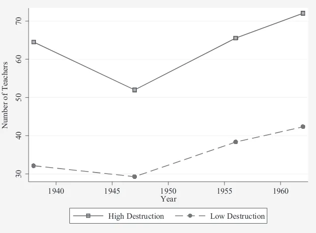
the control group. Figure 1 and Figure 2 show that the schools were rebuilt and the number of teachers reached prewar levels in the early 1960s. These later birth cohorts attained their education after postwar reconstruction; therefore, their human capital
accumulation was not affected by the destruction of WWII.7
5. The statistical signifi cance of difference-in-differences estimates remains unchanged when the standard errors are clustered by region.
6. In Appendix Table A1, I list the number of years that an individual’s education was potentially affected by WWII by an individual’s year of birth. Appendix Table A1 suggests that the educational attainment of cohorts born between 1922 and 1939 were potentially affected by WWII as they were of primary school and upper secondary school age during the war years. If we include individuals who were of college age during WWII, then cohorts born between 1917 and 1939 were potentially affected by WWII.
7. In Appendix Table A2 and Appendix Table A3, I present difference-in-differences estimates with a differ-ent categorization of the affected and the control groups, respectively. The difference-in-differences estimates in these analyses remain economically and signifi cantly similar to the baseline specifi cation.
30
40
50
60
70
N
um
be
r of
S
c
hool
s
1940 1945 1950 1955 1960 Year
High Destruction Low Destruction
Figure 1
Number of Schools by Regional WWII Destruction
In order to interpret β as the effect of war destruction, we must assume that
had WWII destruction not occurred, the difference in schooling, health, and labor market outcomes between the affected and the control groups would have been the same across regions with varying intensity of destruction. I assess the
plausibil-ity of this “parallel trend” assumption below by performing a falsifi cation test/
control experiment by repeating the analysis using only cohorts already beyond school age.
Equation 1 assumes that wartime physical destruction affected the human capi-tal formation of German children who were of school age and has no impact on the educational achievement of earlier and later birth cohorts. To provide more formal
evidence on cohort- specifi c effects of wartime destruction and test the parallel trend
assumption, the identifi cation strategy presented in Equation 1 can be generalized as
follows (Dufl o 2001):
(2) Yirt= α +
c=1 9
∑
(Destructionr × Cohortic)β1c + δr+ γt+ π’X irt+ εirtwhere Yirtis the outcome of interest for individual i in region r, born in year t. Cohortic
is a dummy variable that indicates whether individual i was born in cohort c (a
co-30
40
50
60
70
N
um
be
r of
T
e
ac
he
rs
1940 1945 1950 1955 1960 Year
High Destruction Low Destruction
Figure 2
Number of Teachers by Regional WWII Destruction
hort dummy). To increase statistical precision, birth cohorts are grouped.8
Individu-als born between 1955 and 1960 form the control group, and this cohort dummy is omitted from the regression. These unrestricted estimates in Equation 2 present the
cohort- specifi c impacts of the wartime destruction. Thus, each coeffi cient β1c can be
interpreted as an estimate of the effects of wartime destruction on a given cohort. For the validity of identifying the assumption above, the effects of wartime destruction should be zero or negligible for the cohorts that completed their education before the outbreak of WWII (cohorts born between 1907 and 1916) and for the cohorts starting their education after the reconstruction of school inputs was completed in the early 1960s (cohorts born between 1951 and 1960).
IV. Data and Descriptive Statistics
The measure of WWII destruction intensity that I use for my main anal-ysis is from Kaestner (1949), who reports the results of a survey undertaken by the Ger-man Association of Cities (“Deutscher Staedtetag”). Kaestner provides municipality- level
information on the aggregate residential rubble in m3 per capita accumulated in former
West Germany by the end of WWII.9 In order to examine prewar regional conditions and
assess the mechanisms through which WWII destruction might have affected children’s long- run outcomes, I gathered novel data from various years of the German Municipali-ties Statistical Yearbooks. First, I assembled detailed regional information on the number of schools, teachers, and students to gauge the change in school inputs available to the affected cohorts. Second, I utilized regional data on postwar education and health expen-diture per capita to analyze postwar government spending from various years of German Municipalities Statistical Yearbooks. Additionally, I compiled data on prewar regional characteristics including average income per capita, area, and population density.
The data on individual and household characteristics are from the German Socio- Economic Panel (GSOEP). The GSOEP is a household panel survey that is representa-tive of the entire German population residing in private households. It provides a wide range of information on individual and household characteristics as well as parental background and childhood environment. The GSOEP also incorporates war- related questions including whether an individual’s father was involved in WWII and whether his/her parents died during the war years. In addition, the GSOEP asks respondents
whether they still live in the area where they grew up.10 I restrict the main empirical
8. Appendix Table A1 suggests that individuals born between 1936 and 1939 were of primary school age during WWII. Similarly, the 1931-35 birth cohorts were of primary and lower secondary school age; indi-viduals born between 1925 and 1930 were of lower secondary and upper secondary school age during the war years. Appendix Table A1 also shows that individuals born between 1922 and 1924 were of upper secondary and college age and the 1917-21 cohorts were of college age during WWII. Following the categorization presented in Appendix Table A1, I group the affected birth cohorts accordingly in Table 4.
9. The data on rubble inm3 per capita and population in 1939 are available for almost all towns with 10,000
or more inhabitants in 1939.
analysis to individuals born between 1922 and 1960. I dropped individuals born be-tween 1940 and 1950 from the analysis as they were at school- going age during the reconstruction period that ended in the early 1960s; thus they were partly exposed to
the adverse effects of WWII destruction.11
I consider the effects of WWII at the smallest representative geographical units
(“ROR” or “region”) provided in GSOEP.12 I obtain the historical data set used in
my analysis by compiling the municipality- level data on WWII destruction and other regional macrovariables from the various years of German Municipalities Statistical Yearbooks. I then aggregate these variables according to the 1985 German regional (ROR) boundaries. This aggregation is possible since every municipality reported in the yearbooks belongs to only one ROR. Finally, I merge this aggregated ROR- level
historical data with the 1985 wave of GSOEP by an individual’s ROR.13 I choose the
1985 wave of GSOEP because this is the earliest date both households’ ROR informa-tion and individual and parental characteristics are available. Furthermore, the 1985 wave of GSOEP is only available for former West Germany.
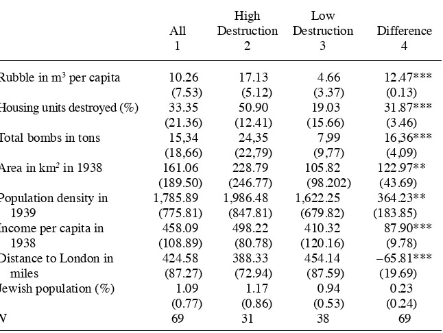
Table 1 presents the descriptive statistics for war destruction measures and variables measuring prewar regional conditions. Table 1 shows that the average West German
region experienced a great deal of destruction: 10.26 rubble in m3 per capita and 33
percent of total housing units were destroyed. There was variation across regions in destruction intensity; regions with above- average destruction had around four times the rubble per capita as regions with below- average destruction. Table 1 also points that highly destroyed regions are larger in area and have higher population density and average income per capita before WWII. Therefore, if we rely only on cross- region variation in destruction to estimate the long- term effects of wartime destruction on
children’s outcomes, it is diffi cult to isolate the effects of destruction from other
specifi c characteristics. The difference- in- differences strategy I propose therefore uses
within- region cross- cohort variation to identify the effects of destruction, and controls
for differences between birth cohorts common across Germany.14
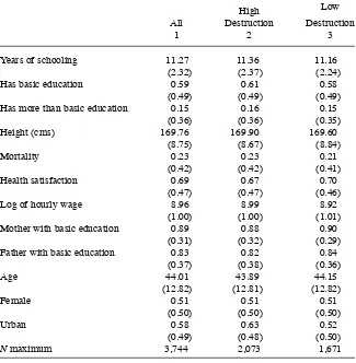
Table 2 shows the descriptive statistics of the outcomes and the main individual- level control variables I use in my estimation. One of the main outcomes of interest is years of schooling completed. The GSOEP asks respondents about educational attainment, then
in the data fi les maps these attainment categories into years of schooling. In addition,
I will analyze health and labor market outcomes. I use three measures of adult health
11. The results for the entire sample, where these 1940-50 cohorts are added to the control group are pre-sented in Column 2 of Appendix Table A3. Point estimate for this specifi cation is smaller in magnitude but statistically similar to the main education results presented in Table 3.
12. These units are called Raumordnungsregionen (RORs) and are determined by the Federal Offi ce for Building and Regional Planning (Bundesamt fuer Bauwesen und Raumordnung, BBR). West Germany has 75 different Raumordnungsregionen. RORs are “spatial districts” based on economic interlinkages and commut-ing fl ows of areas. RORs encompass the aggregation of Landkreise and kreisfreie Städte (Jaeger et al. 2010). 13. The rubble per capita measure is not available for Saar region, which joined West Germany in 1957. Schleswig, Ditmarschen, Emsland, Hochrhein-Bodensee, and Oberland are other RORs with missing wartime destruction data.
including adult height, mortality, and self- reported health satisfaction, and the logarithm of hourly wage as a labor market outcome. These outcomes are measured four decades
after WWII and refl ect the outcomes of WWII survivors who lived to 1985 or later.
V. Estimation Results
A. Educational Attainment
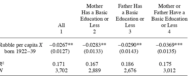
Table 3 reports the results of estimating Equation 1 where the dependent variable is completed years of schooling. Each column is from a separate regression that
con-trols for region and birth year fi xed effects, along with female and rural dummies and
the interaction of the 1939 regional population density with birth year dummies. The
difference- in- differences estimate, β, is reported in the fi rst row. It is negative and
signif-icant at the 95 percent level of confi dence in every specifi cation. Column 1 displays the
difference- in- differences estimate for the entire population. Column 1 has an estimated
β of –0.027, which suggests that school- age children in a region with average
destruc-tion attain 0.3 fewer years of schooling on average. This is the difference- in- differences Table 1
Descriptive Statistics for WWII Destruction
High Low
All Destruction Destruction Difference
1 2 3 4
Rubble in m3 per capita 10.26 17.13 4.66 12.47***
(7.53) (5.12) (3.37) (0.13)
Housing units destroyed (%) 33.35 50.90 19.03 31.87***
(21.36) (12.41) (15.66) (3.46)
Total bombs in tons 15,34 24,35 7,99 16,36***
(18,66) (22,79) (9,77) (4,09)
Area in km2 in 1938 161.06 228.79 105.82 122.97**
(189.50) (246.77) (98.202) (43.69)
Population density in 1,785.89 1,986.48 1,622.25 364.23**
1939 (775.81) (847.81) (679.82) (183.85)
Income per capita in 458.09 498.22 410.32 87.90***
1938 (108.89) (80.78) (120.16) (9.78)
Distance to London in 424.58 388.33 454.14 –65.81***
miles (87.27) (72.94) (87.59) (19.69)
Jewish population (%) 1.09 1.17 0.94 0.23
(0.77) (0.86) (0.53) (0.24)
N 69 31 38 69
coeffi cient β (–0.027) multiplied by the rubble in m3 per capita (10.26m3) in Table 1. To
gain a better understanding on the magnitude of β, we can also compare the educational
attainment of school- aged children who were in Cologne (a heavily destroyed region
with 25.25 m3 rubble per capita) to children who were in Munich (a less- destroyed
region with 6.50 m3 rubble per capita) during WWII.15 Using this comparison, Column
1 suggests that school- aged children in Cologne had 0.5 fewer years of schooling com-pared to the same cohorts in Munich as a result of higher wartime destruction.
15. These two RORs were very similar in terms of their prewar characteristics, but Cologne was closer to bomber aerial fi elds in London and therefore was exposed to higher levels of destruction during WWII. Table 2
Descriptive Statistics, GSOEP Data
High Low
All Destruction Destruction
1 2 3
Years of schooling 11.27 11.36 11.16
(2.32) (2.37) (2.24)
Has basic education 0.59 0.61 0.58
(0.49) (0.49) (0.49)
Has more than basic education 0.15 0.16 0.15
(0.36) (0.36) (0.35)
Height (cms) 169.76 169.90 169.60
(8.75) (8.67) (8.84)
Mortality 0.23 0.23 0.21
(0.42) (0.42) (0.41)
Health satisfaction 0.69 0.67 0.70
(0.47) (0.47) (0.46)
Log of hourly wage 8.96 8.99 8.92
(1.00) (1.00) (1.01)
Mother with basic education 0.89 0.88 0.90
(0.31) (0.32) (0.29)
Father with basic education 0.83 0.82 0.84
(0.37) (0.38) (0.36)
Age 44.01 43.89 44.15
(12.82) (12.81) (12.82)
Female 0.51 0.51 0.51
(0.50) (0.50) (0.50)
Urban 0.58 0.63 0.52
(0.49) (0.48) (0.50)
N maximum 3,744 2,073 1,671
Columns 2–4 of Table 3 present the analysis incorporating family background charac-teristics, such as father’s and mother’s educational attainment, which are likely to serve as a proxy for parents’ economic status. Table 2 indicates that the majority of children have parents with a basic education or less (83 percent of fathers and 89 percent of mothers in my sample completed a basic education or less). Therefore, in Columns 2–4 of Table 3, I focus only on children whose mothers or fathers had a basic school degree (Hauptschule)
or less and estimate the baseline specifi cation only for these children, respectively.16
Re-sults summarized in Columns 2–4 reveal that children with less- educated parents have relatively greater reduction in their educational attainment compared to children with more- educated parents. This differential effect may work literally through parental educa-tion (for example, more- educated parents value educaeduca-tion more and are more able to sub-stitute for missing teachers and so ensure their children are educated too even if negative shocks occur) or through other channels correlated with parental education such as family income or wealth (for instance, rich families can afford to educate their children and can hire private tutors or send children to boarding schools when necessary).
Table 4 presents the cohort- specifi c impacts of the wartime destruction that enable us
to identify the birth cohorts mostly affected by wartime destruction. In addition, Table 4 allows us to formally test the identifying assumption in Equation 1 that assumes that negative effects of wartime destruction are only present for the birth cohorts that were at schoolgoing age during the war years. To increase statistical precision, in Table 4 birth co-horts are grouped following Appendix Table A1. Individuals born between 1955 and 1960 form the control group, and this cohort dummy is omitted from the regression. Table 4 shows that exposure to destruction has substantially deteriorated the human capital forma-tion of cohorts who were of primary school, lower secondary, and upper secondary school age during the war years. Table 4 further reveals that the adverse effects of war shock are
16. The basic school diploma (Hauptschule) is granted after nine years of schooling in Germany. Table 3
Effect of WWII Destruction on Years of Schooling
All
Rubble per capita X –0.0267** –0.0283** –0.0290** –0.0369***
born 1922–39 (0.0127) (0.0133) (0.0143) (0.0135)
R2 0.171 0.167 0.186 0.175
N 3,702 2,889 2,676 3,012
also present for cohorts born between 1936 and 1939; although it seems that these younger cohorts who were only of primary school age by the end of WWII were more resilient to wartime destruction. Additionally, Table 4 reports that wartime destruction has no effect on the human capital formation of the earlier and the later birth cohorts. This supports the aforementioned identifying assumption and suggests that the estimation results presented
in Table 3 are not confounded by prewar and postwar region- specifi c cohort trends.
A potential confounding factor for the foregoing results on the effect of wartime de-struction on education is the possibility of nonrandom migration across regions. People residing in heavily destroyed areas may have been displaced to less destroyed areas dur-ing heavy aerial attacks. Alternatively, highly destroyed areas may have attracted a large number of postwar economic migrants seeking to take part in reconstruction efforts. Both types of migration may induce selection bias in the analysis of WWII destruction effects on children’s long- term outcomes. To address whether an individual’s migra-tion decision is based on destrucmigra-tion intensity, I estimate Equamigra-tion 1 using the prob-ability of moving as the dependent variable. Results are reported in Table 5, Panel A. Individuals are coded as movers if they report that they no longer reside in their
child-Table 4
Effect of WWII Destruction on Years of Schooling by Cohorts
Rubble per capita X born 1907–11 0.007
(0.027)
Rubble per capita X born 1912–16 –0.024
(0.021)
Rubble per capita X born 1917–21 –0.027
(0.020)
Rubble per capita X born 1922–24 –0.046**
(0.023)
Rubble per capita X born 1925–30 –0.033*
(0.019)
Rubble per capita X born 1931–35 –0.041**
(0.021)
Rubble per capita X born 1936–39 –0.025
(0.019)
Rubble per capita X born 1940–44 –0.023
(0.018)
Rubble per capita X born 1945–49 –0.005
(0.022)
Rubble per capita X born 1950–54 0.001
(0.022)
R2 0.1560
N 6,265
hood area in 1985. The affected and the control groups for this specifi cation are the same as in the Table 3 education analysis. The difference- in- differences estimates for
probability of moving are close to zero and statistically insignifi cant at the
conven-tional level in every specifi cation. This fi nding suggests that individuals did not choose
their fi nal destination according to regional destruction.17
17. An additional concern related to mobility is refugees or people who fl ed from the former parts of Ger-many and Soviet Zone/GDR. As an attempt to address this potential concern, I use the offi cial 1961 refugee data kindly provided by Redding and Sturm (2008) and estimate the baseline specifi cation separately for regions with refugees above and below median. I fi nd similar effects for both samples.
Table 5
Validity Checks
All Mother
Has a Basic Education or
Less
Father Has a Basic Education or
Less
Mother or Father Have a Basic Education
or Less
1 2 3 4
Panel A: Effect of WWII Destruction on Probability of Moving
Rubble per capita X 0.002 0.005 0.004 0.005
born 1922–39 (0.003) (0.003) (0.003) (0.003)
R2 0.112 0.125 0.134 0.122
N 3,700 2,890 2,675 3,013
Panel B: Nonmovers Only
Rubble per capita X –0.035*** –0.034** –0.026* –0.038**
born 1922–39 (0.013) (0.015) (0.015) (0.015)
R2 0.212 0.207 0.237 0.214
N 2,025 1,621 1,530 1,690
Panel C: Control Experiment
Rubble per capita X 0.004 0.029 0.009 0.029
born 1907–11 (0.025) (0.028) (0.026) (0.028)
R2 0.305 0.323 0.32 0.31
N 644 491 466 499
Panel B in Table 5 provides further evidence on the lack of nonrandom migration. The analysis in Panel B is restricted to individuals who still live in the area where they grew up (hereafter, “nonmovers”). The difference- in- differences estimates for nonmovers are very similar to the estimates for the entire population (difference- in- differences estimates for the entire population and nonmovers lie within each other’s
95 percent confi dence intervals). The empirical evidence presented in Panel B
sup-ports previous fi ndings that nonmovers are not differentially affected by the war shock
and suggests that the nonrandom migration is unlikely to be a concern.
Results presented in Table 3 rest on the assumption that in the absence of WWII, the difference in educational attainment between the affected group and the later birth cohorts would have been similar across regions with varying intensity of destruction.
That is, the coeffi cient for interaction between being born between 1922 and 1939 and
regional rubble in m3 per capita would be zero in the absence of WWII destruction.
However, if there were differential cohort trends in educational attainment between more destroyed and less destroyed regions, then it would not be possible to interpret the difference- in- differences estimates as due to WWII destruction. To assess the validity
of the identifying assumption, I perform the following falsifi cation test/control
experi-ment. I restrict the empirical analysis to older cohorts who would have completed their schooling at the outset of WWII. The oldest cohorts (individuals born between 1907 and 1911) are coded as the “Placebo” affected cohort and cohorts born between 1912 and 1916 as the “Placebo” control cohort, although of course there is no true treatment here. If there are no differential trends, then the difference- in- differences estimates
should be zero, which is indeed what I fi nd (See Panel C in Table 5). These results
lend further credence to the identifi cation assumption in Equation 1 and support the
interpretation of the difference- in- differences estimates as due to WWII destruction
as opposed to some region- specifi c cohort trend.
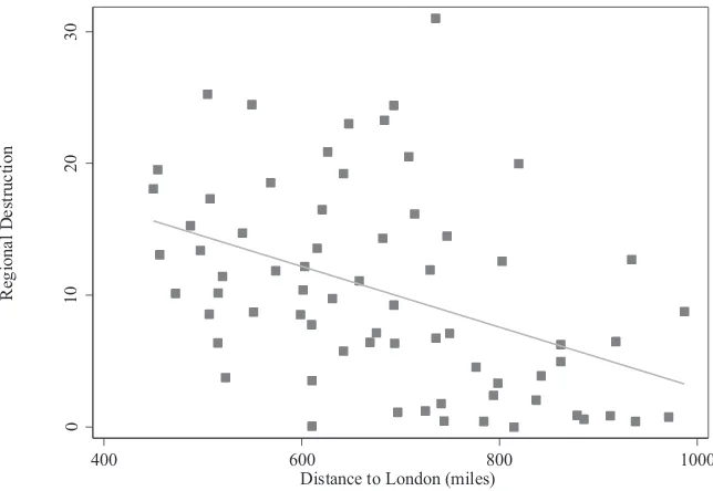
An additional concern for the parallel trend assumption is that WWII destruction may be endogenous to trends in children’s education, or the distribution of postwar reconstruction efforts may be endogenous. That is, it is possible that the postwar re-construction efforts were unevenly allocated toward areas with better growth pros-pects. To address this potential concern, I employ an instrumental- variable strategy. The instrumental variable that I use for wartime physical destruction is distance to London obtained using the Geographic Names Information System (GNIS). As stated in Section II, the northern and western parts of Germany suffered the most from AAF aerial bombing. Therefore, distance to London should be a good predictor of the war destruction experienced in each German region. Figure 3 illustrates the association between region’s distance to London and war destruction. Consistent with the histori-cal sources, Figure 3 indeed shows that regions closer to London experienced more destruction as a result of AAF aerial raids.
Table 6 provides more formal evidence on instrumental- variable estimates.18 The lower
panel in Column 1 shows that the fi rst- stage estimates are statistically signifi cant at 1
percent signifi cance level consistent with the hypothesis that regions further away from
London were exposed to considerably less destruction during WWII. The results from
estimating Equation 1 using two- stage least squares are given in upper panel of Column 1. The 2SLS estimate indicates that, on average, children completed 0.5 fewer years of schooling as a result of WWII devastation. This is larger in magnitude than the original difference- in- differences estimates presented in Table 3, although it should be noted that
the standard errors for the 2SLS estimates are also larger.19 This
fi nding further bolsters
the idea that WWII destruction is exogenous once I control for region fi xed characteristics.
As summarized in Table 6, German regions closer to airfi elds in England suffered
the most from AAF bombing campaign during WWII, which may raise potential con-cerns on differential postwar cohort trends in educational attainment across regions with varying distance to London. That is, German states closer to England such as Schleswig- Holstein, Hamburg, Lower Saxony, and North Rhine- Westphalia were mainly occupied by British forces and may have experienced different postwar edu-cational policies compared to German states in the south and southwest occupied by the U.S. and French forces. The extent of such potential bias is largely mitigated by the fact that I use a lower level of aggregation than state in estimating the long- term
19. In Table 6, I report the statistics of weak identifi cation test. The value of weak identifi cation test (Klei-bergen-Paap rk Wald F-statistics) is 1196.14. The Stock-Yogo critical value for one endogenous variable and one instrument is 16.38 for 10 percent maximal IV size. In Table 6, I also present the statistics for two weak-instrument-robust-inference tests. The Chi-square statistics for Anderson-Rubin Wald test is 5.67. Similarly, the Chi-square statistics for the Stock-Wright LM S statistic is 5.53. Both Chi-square values are greater than Chi-square (1) critical value of 3.841 at the 5 percent signifi cance level. Therefore, the proposed instrument, “distance to London” passes both weak identifi cation tests and weak-instrument-robust inference tests.
0
10
20
30
Re
gi
ona
l D
e
st
ruc
ti
on
400 600 800 1000
Distance to London (miles)
Figure 3
effects of wartime destruction, which allows me to explore within state variation in
wartime destruction. Thus, I can account for postwar state- specifi c education policies
in my analysis. Moreover, the difference- in- differences estimates remain virtually
unchanged in specifi cation controlling for state- specifi c trends, as reported in Column
1 of Table 7. As further evidence on the lack of differential postwar time trends in education, I compiled regional data on postwar education expenditure per capita from
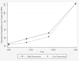
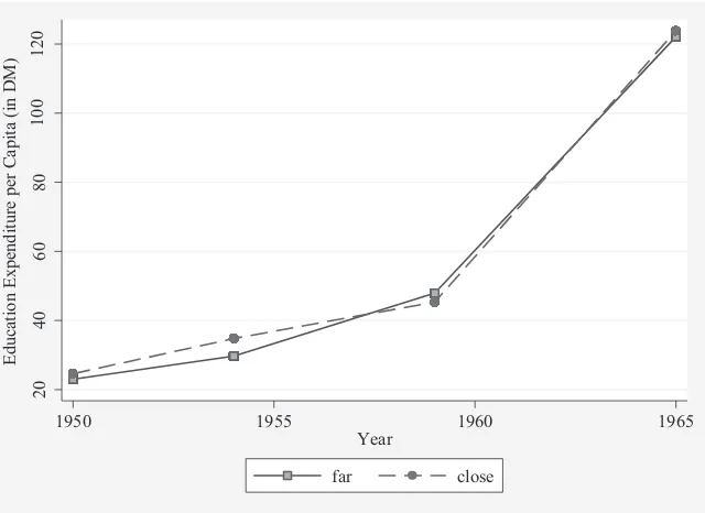
various years of German Municipalities Statistical Yearbooks. 20 Analyses using this
data reveal that there are no postwar differential time trends in per capita education expenditure for the control cohorts residing in highly destroyed regions as well as in regions closer to London. (See Figure 4 and Figure 5.) Taken together, these additional analyses suggest that postwar differential time trends in educational attainment are unlikely to be a concern and further support the parallel trend assumption underlying Equation 1.
Another potential confounding factor is the differential exposure to the dismissal and exile of the Jewish population during the Nazi Regime across German regions
20. I generate fi gures on education expenditure using information on 1950, 1954, 1959, and 1965 fi scal years. Table 6
The Effect of WWII Destruction on Years of Schooling, IV Results
Second- Stage Reduced- Form
1 2
Rubble per capita X born 1922–39 –0.0516**
(0.0218)
Distance to London X born 1922–39 0.0023**
(0.0010)
First- Stage
Dependent Variable: Rubble per Capita X born 1922–39
Distance to London X born 1922–39 –0.0443***
(0.0023)
Kleibergen- Paap rk Wald statistics 1,196.14
Anderson- Rubin Wald test (Chi- square) 5.67
Stock- Wright LM S statistic 5.53
N 3,702
651
Source of Heterogeneity Destruction Measure
State Trends
Males Only
Urban Area Only
Top Quartile Destruction
Parent Died During WWII
Father Fought in
WWII
School Destruction
Missing Teachers
Number of Years Exposed
(1) (2) (3) (4) 5 6 7 8 9
Rubble per capita X –0.0262** –0.0423** –0.0404** –0.7575*** –0.0276** –0.0245* –0.0243* –0.0251**
born 1922–39 (0.0127) (0.0187) (0.0178) (0.2434) (0.0127) (0.0138) (0.0130) (0.0129)
Mother died during –0.6602*** –0.6859***
WWII (0.2062) (0.2078)
Father died during 0.0493 (0.0074)
WWII (0.1470) (0.1474)
Father fought in –0.5579***
WWII (0.1556)
Percentage of schools –0.0108**
destroyed X born 1922–39 (0.0045)
Percentage of missing –0.0019
teachers X born 1922–39 (0.0046)
Rubble per capita X Number –0.0046**
of years Exposed to WWII (0.0023)
R2 0.162 0.151 0.157 0.173 0.172 0.183 0.172 0.172 0.17
N 3,702 1,805 2,140 3,702 3,702 3,396 3,523 3,523 3,702
with varying intensity of wartime destruction. Hitler’s Nazi Party passed the “Law for the Restoration of the Professional Civil Service” shortly after they came into power in 1933. This law allowed the Nazi government to purge the Jewish population from the civil service, a vast organization in Germany that included teachers, professors, judges, and many other professionals. The nationwide effects of the persecution of the
Jewish population are captured by the birth year fi xed effects in my analysis. However,
if regional wartime destruction is associated with the Jewish population, this may raise potential concerns on the interpretation of my analyses. Table 1 shows that the faction of Jewish population is similar across regions; therefore, it is unlikely that the results
are confounded by the differential Jewish population.21
Finally, analyses presented in Appendix Table A2 and Appendix Table A3 suggest that the main education results presented in Table 3 are robust to the different categorization of the affected and the control cohorts. In Column 1 of Appendix Table A2, the affected cohorts
21. In addition, I estimate an additional sensitivity analysis that includes the interaction of the change in the Jewish population residing in each German region with being in the affected cohort as an additional control to the baseline specifi cation. The difference-in-differences estimates remain quantitatively and statistically similar in this specifi cation, which provides further evidence that the empirical analyses presented in the paper are not confounded by the persecution of the Jewish population.
20
Postwar per Capita Education Expenditure by WWII Destruction
encompass individuals born between 1917 and 1939. This is the most inclusive defi ni-tion of the affected group. These cohorts were of primary school and college age during WWII; therefore, at least one year of the educational attainment of these cohorts had po-tentially been interrupted by WWII. In Column 2, I present the difference- in- differences estimates with the affected cohorts used in the main analysis in Table 3. In Column 3, I
defi ne the affected cohorts as individuals born between 1927 and 1939. These cohorts
were between 6 and 18 years old by the end of WWII in 1945. In the last column of Ap-pendix Table A2, individuals born between 1930 and 1939 constitute the affected cohorts.
This is the most conservative defi nition of the affected group. These individuals were at
the compulsory schooling age or younger by the end of WWII. In all columns in Appen-dix Table A2, the difference- in- differences estimates remain quantitatively and
statisti-cally similar to the baseline specifi cation presented in Table 3.
Appendix Table A3 reports the difference- in- differences estimates for educational attainment with a different categorization of the control group. In Column 1, the
control group is defi ned as individuals born between 1907 and 1916. These cohorts
were 23 years old and older when WWII started on September 1939 (beyond college
age); therefore their schooling was not potentially affected by WWII destruction.22 In
Column 2, individuals born between 1940 and 1960 form the control cohorts. These
22. However, these cohorts attained part of their education during WWI.
20
Postwar per Capita Education Expenditure by Distance to London
cohorts attained their educational attainment after WWII but some of these cohorts started school in the 1940s and 1950s before the postwar reconstruction was over in Germany. In Column 3, the 1947–60 birth cohorts encompass the control cohorts. The last column of Appendix Table A3 displays the difference- in- differences anal-ysis with individuals born between 1951 and 1960 in the control group. These are also the control cohorts used in the main analysis. These cohorts started school after postwar reconstruction was over in the early 1960s; therefore, their educational at-tainment was not potentially affected by WWI, WWII, or postwar reconstruction. The difference- in- differences estimates in Appendix Table A3 are statistically and quanti-tatively similar to the main results presented in Table 3, which suggests that the main education results also hold with a different categorization of the control group.
B. Potential Mechanisms
In this subsection, I investigate the potential heterogeneous effects of WWII and pro-vide formal epro-vidence on the mechanisms through which war destruction affected the children’s educational attainment. The results are summarized in Table 7. In Column 1, I formally test whether my results are sensitive to the inclusion of the linear state- cohort trends. The difference- in- differences estimate remains virtually unchanged when I
con-trol for state- specifi c trends suggesting that the results are not confounded by postwar
state- specifi c education policies. In Columns 2 and 3, I restrict the analysis only to males
and individuals residing in urban areas, respectively. I fi nd that difference- in- differences
estimates for males and the urban population are not statistically signifi cantly different
than the estimates for the entire population. The difference- in- differences estimates
for both analyses lie within 95 percent confi dence intervals of the entire population.
On the other hand, one may expect the effect of war destruction to be nonlinear, which suggests that, when destruction surpasses a certain level, otherwise modest or negligible detrimental effects become especially large. The quartile analysis reported in Column 4 shows that children in most hard- hit areas attain 0.8 fewer years of schooling relative to the control group; this effect is twice as large as for the second and bottom quartiles.
In Columns 5 and 6, I introduce war- related controls to the baseline specifi cation such
as whether father actively fought in the war and loss of a parent during the war years to
account for the family’s fi rsthand experience with the consequences of the war. The
re-sults are basically unchanged, controlling for a parent fi ghting in WWII or dying during
WWII years, which suggests that it is not the direct family experience in WWII combat that is responsible for the effects on children’s schooling. A more likely mechanism seems to be the destruction of schools and the disruption in schools left standing. Figure 1 and Figure 2 show the decline in the number of schools and teachers over time by
war-time destruction intensity in each region. From these fi gures, it appears that regions with
more rubble per capita also had a greater decline in both the number of schools (because schools were also destroyed as part of the AAF bombing) and the number of teachers
(some teachers had to perform military service and a signifi cant number were Jewish).
measures of war devastation in addition to wartime destruction. In Column 7, the difference- in- differences estimate for rubble per capita decreases by 10 percent
com-pared to the baseline specifi cation in Table 3 once I control for the interaction between
the decrease in the number of schools per student during WWII and an indicator for being in the affected group. This suggests that 10 percent of the total effect can be
ex-plained by school destruction. Similarly, in Column 8, I estimate the baseline specifi
-cation controlling for the interaction between the decline in the number of teachers per student during WWII and for being in the affected group. The difference- in- differences estimate for wartime destruction drops by 6 percent in Column 8, which suggests that 6 percent of the total destruction effect is associated with missing teachers. These columns evidently point out that the destruction of schools has enduring detrimental effects. However, it also seems that the extensive AAF bombings limited the children’s access to education even though the schools were intact.
Lastly, WWII_Cohortit can be defi ned as number of years that an individual’s
ed-ucational attainment was affected by exposure to war destruction. To generate this variable, I assume that individuals’ educational attainment was impacted by WWII destruction if they were of primary school and upper secondary school during the war
years.23 Column 9 presents this alternative speci
fi cation where wartime destruction is
interacted with the number of years that an individual’s education was interrupted by
WWII. Similar to the main education results presented in Table 3, in Column 9, I fi nd
that school- aged children in a region with average destruction attain 0.3 fewer years of schooling on average if they were school- aged during the entire duration of WWII.
This is the difference- in- differences coeffi cient β (–0.0046) multiplied by the average
population- weighted rubble in m3 per capita (10.26m3) in Table 1 and the duration of
WWII. These additional analyses show that the estimation results presented in Table 3 also hold when the destruction variable is interacted with a continuous measure of the number of school- age years a cohort was exposed to war.
C. Health Outcomes
Now, I turn to estimations on the impact of WWII destruction on individuals’ adult health outcomes. The health outcomes that I analyze are height, mortality, and health satisfaction. A mediator for long- run health effects, especially height in adulthood, is childhood nutritional status. WWII created food shortages and changes in the compo-sition of food eaten that could have had especially detrimental effects on young chil-dren. The affected and the control groups described above for the education analysis apply just as well for health outcomes, with the exception of height.
Table 8 reports the difference- in- differences estimates for adult health outcomes. Panel A examines the effect of WWII destruction on individual height (measured in
inches). The cohort- specifi c analysis presented in Appendix Table A4 suggests that
chil-dren who were born between 1935 and 1944 were primarily affected by the adverse im-pacts of war devastation on adult height. Thus, for height regressions, the affected group is restricted to individuals who were born between 1935 and 1944, that is, a dummy
variable WWII_Cohortit takes a value of 1 if individual i was born between 1935 and
1944, and zero otherwise. All specifi cations in Panel A show that wartime destruction
had a long- lasting, detrimental effect on adult height. The difference- in- differences estimate in Column 1 is –0.06 indicating that individuals who grew up in a region with average destruction are approximately 0.6 inches shorter on average in adulthood than
the others.24 Alternatively, in the comparison of Cologne and Munich, wartime children
residing in Cologne had an inch lower height in their adulthood relative to the same cohorts in Munich. This is a sizable effect as average height increased by only 0.8 inch
in the entire 19th century in France (Banerjee et al. 2010).
Panel B presents the results for the mortality of WWII survivors. For this analysis,
24. The instrumental variable estimate for adult height is -0.12 with the standard error of 0.04. These results are available upon request.
Table 8
Effects of WWII Destruction on Adult Health Outcomes
All
Rubble per capita X –0.0577*** –0.0478** –0.0429** –0.0472**
born 1935–44 (0.0200) (0.0206) (0.0215) (0.0209)
R2 (0.5570) 0.582 0.564 0.57
N 1,373 1,137 1,046 1,194
Panel B: Mortality
Rubble per capita X 0.0004 0.0021 0.0043** 0.0027
born 1922–39 (0.0016) (0.0019) (0.0020) (0.0019)
R2 0.268 0.267 0.279 0.269
N 3,717 2,902 2,686 3,025
Panel C: Self- Rated Health Satisfaction
Rubble per capita X –0.0009 –0.0053** –0.0057** –0.0051**
born 1922–39 (0.0022) (0.0024) (0.0025) (0.0024)
R2 0.111 0.123 0.141 0.122
N 3,699 2,889 2,677 3,011
I take advantage of the panel structure of GSOEP, which enables me to analyze the longer- run consequences of warfare. The mortality variable is a dummy variable that takes a value of 1 if an individual has a recorded death year sometime between 1985
(the beginning of my sample) and 2011, and zero otherwise.25 The results reported in
Panel B provide suggestive evidence that WWII destruction caused Germans who were school- aged during WWII to die sooner; however, the difference- in- differences
estimate is statistically signifi cant only for children with less educated fathers.
Finally, Panel C estimates the effect of war destruction on self- reported health
satis-faction in adulthood. Health satissatis-faction is often considered to have signifi cant
explana-tory power in predicting future mortality and is therefore a useful measure of morbidity (Idler and Benysmini 1997; Frijters, Haisken- DeNew, and Shields 2011). Health sat-isfaction in the GSOEP is measured on a scale from 0 to 10. Individuals are coded as
satisfi ed with their current health if their response is 6 and above. The results in Panel
C are negative and signifi cant, suggesting that exposure to warfare reduces
satisfac-tion with current health among children from disadvantaged families by six percentage points on average. Thus, war destruction does worsen long- run health status.
D. Labor Market Outcomes
In this subsection, I analyze the effects of WWII devastation on an individual’s future labor market outcomes. Given well- established empirical evidence on the causal as-sociation between individuals’ human capital, health status, and labor market out-comes (Card 1999; Case and Paxson 2008), wartime physical destruction can impact individuals’ future labor market outcomes through reduction in educational attainment (as summarized in Table 3) or through other channels, including deterioration in adult-hood health (as reported in Table 8).
The outcome of interest in Table 9 is the logarithm of hourly wage. This analysis is
restricted to individuals with positive labor market earnings in 1985.26 Females have
signifi cantly lower labor force participation rates than males in Germany (Bonin and
Rob Euwals 2005; Strøm and Wagenhals 1991); therefore, I allow the treatment effect to differ by gender in Table 9. Table 9 shows that males from disadvantaged families residing in a region with average wartime destruction earn about 9 percent less on average in adulthood. On the other hand, it appears that the adverse effects of wartime
destruction on female long- term labor market earnings are limited.27
VI. Conclusion
This paper presents causal evidence on the long- run socioeconomic con-sequences of large- scale physical destruction arising from the world’s most costly and
widespread global military confl ict, World War II. The fi ndings in this paper shed light on
potential long- term legacies of large- scale physical destruction that could be caused by
nat-25. Information on an individual’s death year in GSOEP comes from offi cial vitality records. 26. I fi nd similar results when I include zero wages into the analysis.
ural disasters and armed confl icts experienced in many countries around the globe. I com-bine a detailed data set on regional WWII destruction in Germany with individual- level data from the GSOEP to study the long- run effects of wartime physical destruction on
German children’s education, health, and labor market outcomes. The identifi cation
strat-egy exploits plausibly exogenous region- by- cohort variation in the intensity of WWII
destruction. I fi nd that WWII destruction caused Germans who were school- aged during
WWII to complete fewer years of schooling, be shorter in height, report lower satisfaction with their current health, die sooner, and have lower labor market earnings in the future.
The formal analysis of mechanisms suggests that the destruction of schools has en-during detrimental effects. However, it also seems that extensive AAF bombings lim-ited the children’s access to education even though school buildings were left intact. In addition, given the sizable destruction effects on height, it seems that malnutrition is partly behind the estimated impact on long- term health. Other factors, however, such as pollution, lack of clean water, and limited access to health facilities may also be responsible for the health results.
Findings in this paper suggest that even though severely hit regions rapidly returned to their prewar patterns in terms of macroeconomic indicators and physical
infrastruc-ture as shown in previous studies, the consequences of armed confl icts are more
sub-stantial and long- lasting along human dimensions. Given that the detrimental effects of WWII destruction on individuals’ education, health, and labor market outcomes are still present four decades after WWII, these results underline the importance of poli-cies primarily targeting children after large- scale physical destruction.
Table 9
Effect of WWII Destruction on Logarithm of Hourly Wage
All
Rubble per capita X –0.0042 –0.0026 –0.0092* –0.005
born 1922–39 (0.0057) (0.0047) (0.0054) (0.0051)
Rubble per capita X 0.0046 –0.0122 0.0054 0.002
born 1922–39 X
Female
(0.0134) (0.0151) (0.0171) (0.0157)
R2 0.392 0.44 0.457 0.424
N 2,288 1,790 1,636 1,873
Appendix
Table A1
The Number of Years Affected from WWII
Table A2
Effects of WWII Destruction on Years of Schooling by Different Affected Groups
Affected Group
Born Born Born Born
1917–39 1922–39 1927–39 1930–39
(1) (2) (3) (4)
Rubble per capita X –0.0347*** –0.0369*** –0.0313** –0.0362**
Cohort dummy (0.0133) (0.0135) (0.0140) (0.0144)
R2 0.176 0.175 0.168 0.166
N 3,305 3,012 2,595 2,288
Notes: Standard errors clustered by region and birth years are shown in parentheses. Asterisks denote sig-nifi cance levels (*=0.10, **=0.05, ***=0.01). The control group is individuals born between 1951 and 1960. Each column controls for region and year of birth- fi xed effects. Other controls in each regression are gender and rural dummies and the interaction of prewar regional population density with birth- year dummies.
Table A3
Effects of WWII Destruction on Years of Schooling by Different Control Groups
Control Group
Born Born Born Born
1907–16 1940–60 1947–60 1951–60
(1) (2) (3) (4)
Rubble per capita X born –0.0304** –0.0261** –0.0348*** –0.0369***
1922–39 (0.0139) (0.0105) (0.0123) (0.0135)
R2 0.209 0.157 0.168 0.175
N 2,161 4,197 3,461 3,012
References
Akresh, Richard, and Damien de Walque. 2008. “Armed Confl ict and Schooling: Evidence from the 1994 Rwanda Genocide.” Households in Confl ict Network Working Papers 47. Alderman, Harold, John Hoddinott, and Bill Kinsey. 2004. “Long Term Consequences of Early
Childhood Malnutrition.” Oxford Economic Papers 58(3):450–74.
Angrist, Joshua and Adriana Kugler. 2008. “Rural Windfall or Resource Curse? Coca, Income and Civil Confl ict in Colombia.” Review of Economics and Statistics 90(2):191–215. Banerjee, Abhijit, Esther Dufl o, Gilles Postel- Vinay, and Tim Watt. 2010. “Long Run Health
Impacts of Income Shocks: Wine and Phylloxera in Nineteenth- Century France.” Review of Economics and Statistics 92(4):714–28.
Blattman, Christopher, and Edward Miguel. 2010. “Civil War.” Journal of Economic Litera-ture 48(1):3–57.
Bonin, Holger, and Rob Euwals. 2005. “Why Are Labor Force Participation Rates of East Ger-man Women So High?” Applied Economics Quarterly 51(4):359–86.
Brakman, Steven, Harry Garretsen, and Marc Schramm. 2004. “The Strategic Bombing of Cities in Germany in World War II and Its Impact on City Growth.” Journal of Economic Geography 4(1):1–18.
Table A4
Effects of WWII Destruction on Height by Cohorts
Rubble per capita X born 1925–29 0.0386
(0.0325)
Rubble per capita X born 1930–34 –0.0571
(0.0340)
Rubble per capita X born 1935–39 –0.0746***
(0.0270)
Rubble per capita X born 1940–44 –0.0560**
(0.0275)
Rubble per capita X born 1945–50 –0.0119
(0.0298)
Rubble per capita X born 1951–55 –0.0218
(0.0291)
R2 0.548
N 2,197