Full Terms & Conditions of access and use can be found at
http://www.tandfonline.com/action/journalInformation?journalCode=ubes20
Download by: [Universitas Maritim Raja Ali Haji] Date: 11 January 2016, At: 23:00
Journal of Business & Economic Statistics
ISSN: 0735-0015 (Print) 1537-2707 (Online) Journal homepage: http://www.tandfonline.com/loi/ubes20
Autocontours: Dynamic Specification Testing
Gloria González-Rivera, Zeynep Senyuz & Emre Yoldas
To cite this article: Gloria González-Rivera, Zeynep Senyuz & Emre Yoldas (2011) Autocontours: Dynamic Specification Testing, Journal of Business & Economic Statistics, 29:1, 186-200, DOI: 10.1198/jbes.2010.08144
To link to this article: http://dx.doi.org/10.1198/jbes.2010.08144
View supplementary material
Published online: 01 Jan 2012.
Submit your article to this journal
Article views: 85
Supplementary materials for this article are available online. Please click the JBES link athttp://pubs.amstat.org.
Autocontours: Dynamic Specification Testing
Gloria G
ONZÁLEZ-R
IVERADepartment of Economics, University of California, Riverside, Riverside, CA 92521 (gloria.gonzalez@ucr.edu)
Zeynep S
ENYUZDepartment of Economics, University of New Hampshire, Durham, NH 03824 (zeynep.senyuz@unh.edu)
Emre Y
OLDASDepartment of Economics, Bentley University, Waltham, MA 02452 (eyoldas@bentley.edu)
We propose a new battery of dynamic specification tests for the joint hypothesis of iid-ness and density function based on the fundamental properties of independent random variables with identical distributions. We introduce a device—the autocontour—whose shape is very sensitive to departures from the null in either direction, thus providing superior power. The tests are parametric with asymptotictand chi-squared limiting distributions and standard convergence rates. They do not require a transformation of the original data or a Kolmogorov style assessment of goodness-of-fit, explicitly account for parameter uncertainty, and have superior finite sample properties. An application to autoregressive conditional duration (ACD) models for trade durations shows that the difficulty with the assumed densities lies on the probability assigned to very small durations. Supplemental materials for this article are available online.
KEY WORDS: Autoregressive conditional duration model; Bootstrap; Parameter uncertainty; Probabil-ity contour plot.
1. INTRODUCTION
We propose a new battery of tests for dynamic specifica-tion that rely on the fundamental properties of independent ran-dom variables with identical distributions. We focus on mod-els in which all the dependence is contained in the first and second moments such that for a process {yt} we have yt = μt(θ01,ℑt−1)+σt(θ02,ℑt−1)εt whereμt(·)is the conditional mean and σt2(·)is the conditional variance, both functions of an information setℑt−1,θ0=(θ′01,θ′02)′is a parameter vector, andεtis an innovation that is iid. The innovationεtis character-ized by a parametric pdf, sayf(εt). In this context, we formulate a collection of statistics for the joint hypothesis of iid-ness and density functional form of the innovation as specification tests of the full model.
There is an extensive literature on testing a single hypoth-esis, either density functional form or iid behavior. There are numerous parametric and nonparametric tests for density func-tional form, most of which assume iid observations as a starting point as inAndrews(1997), or independence as inFernandes and Grammig(2005). On the other hand, there are several diag-nostic checks that do not explicitly consider the density func-tional form. Brock et al. (1996), Hong and Lee(2003), and Chen(2008), among others, test for iid-ness,Escanciano(2008) focused on the specification of conditional mean and variance, andMeitz and Terasvirta(2006) provided Lagrange multiplier (LM) tests of dependence in the context of duration models. Testing thejointhypothesis of iid-ness and density functional form arise concurrently with the interest in density forecast evaluation methods based on Rosenblatt’s probability integral transform. If the proposed density forecast, sayft(·), is correct, then the transformed random variables, ut=Ft(yt|ℑt−1;θ0), are iid uniformly distributed, see Diebold, Gunther, and Tay (1998), Berkowitz (2001), Chen and Fan (2004), who tested the joint hypothesis of iid-ness and uniformity without account-ing for parameter uncertainty. Bai(2003) dealt with parame-ter uncertainty, but his test lacks power against violations of
independence (seeCorradi and Swanson 2006).Hong and Li (2005) proposed a nonparametric-kernel-based test statistic that has power against violations of both independence and density functional form. Their procedure is asymptotically distribution free, but it is dependent on the choice of the bandwidth.
In this article we propose a battery of tests for the joint hy-pothesis of iid-ness and density functional form that are very powerful against violations of both. The proposed tests focus on fundamental properties of independent random variables with identical distributions. Let the process under consideration be{εt}with densityf(·). The random variables in this process are independent if and only if their multivariate distribution is equal to the product of their marginal distributions, in which case the null hypothesis simply boils down tof(εt−k1, εt−k2,
. . . , εt−km) = f(εt−k1)f(εt−k2)· · ·f(εt−km), {kj}
m
j=1 ∈ N. The specification tests we propose are based on a new concept that we termautocontour. Under the null, we horizontally slice the joint density at different levels and project the resulting seg-ments down to the hyperplane (εt−k1, εt−k2, . . . , εt−km). The projection is the autocontour containing a known percentage of the observations. Based on the sample estimates of these per-centages we construct a battery oft-statistics and chi-squared statistics, which have standard asymptotic distributions. The shape of the autocontour will change whenever there is a de-parture from the null in any direction, and by doing so it will provide superior power to the tests. Our tests can be applied to primitive series and model residuals, in which case we need to address the parameter uncertainty problem. We show that a gen-eral bootstrap procedure to obtain asymptotic variance matrices delivers standard asymptotic tests with very good finite sample
© 2011American Statistical Association
Journal of Business & Economic Statistics
January 2011, Vol. 29, No. 1 DOI:10.1198/jbes.2010.08144
186
performance. In comparison with the existent tests, the autocon-tour tests have several advantages as they are parametric with standard convergence rates and standard limiting distributions that deliver superior power. They are computationally easy to implement as they are based on counting processes. In addition, they do not require either a transformation of the original data or an assessment of Kolmogorov goodness-of-fit, and explicitly account for parameter uncertainty.
The structure of the article is as follows. In Section2, we formalize the notion of autocontour and present the testing methodology. In Section3we explicitly deal with the parame-ter uncertainty problem. In Section4, we provide Monte Carlo evidence on the size and power properties of our tests and of-fer a comparison with the nonparametric tests ofHong and Li (2005). Section5contains an empirical application in the con-text of autoregressive conditional duration (ACD) models. We conclude in Section6. All mathematical proofs can be found in Appendix B.
2. THE JOINT TEST OF DENSITY AND INDEPENDENCE
The class of dynamic models that we are interested in are of the following form:
yt=μt(θ01,ℑt−1)+σt(θ02,ℑt−1)εt, t=1, . . . ,T, (2.1) whereℑt−1denotes the information set available at timet−1, μt(·)andσt(·)are fully parameterized byθ0=(θ′01,θ′02)′ and measurable with respect to ℑt−1, and{ε}Tt=1 is a series of iid innovations having a particular density functionf(·). Usually, εtis assumed to have zero mean and unit variance, but for non-negative data it will naturally have a nonzero mean. We assume first thatεt is observable, i.e.,θ0 is known. Later on we will relax this assumption to account for the effects of estimation on the distribution of our test statistics.
2.1 Autocontour
Under correct dynamic specification the null hypothesis in its most general form is stated as, H0:εt is iid with density f(·), whereH1is the negation ofH0. Under this null hypoth-esis the multivariate density function for an m-dimensional vector(εt−k1, εt−k2, . . . , εt−km)is written asf(εt−k1, εt−k2, . . . ,
εt−km)= f(εt−k1)f(εt−k2)· · ·f(εt−km). We define the (α,m) autocontour, ACRmα, as the set of points in the hyperplane (εt−k1, εt−k2, . . . , εt−km) that results from horizontally slicing the multivariate density function at a fixed value, say fα, to guarantee that the resulting set contains α% of observations, that is,
Our testing methodology focuses on the bivariate autocon-tour because, as we will show in the forthcoming sections, the tests enjoy superior power in the most empirically rele-vant cases. Monte Carlo simulations illustrate the consistency of the tests against a wide set of alternatives. Tests based on higher-dimensional autocontours can deliver more power, but at the cost of higher-dimensional integration problems in the con-struction of the autocontour and loss of the graphical represen-tation that is useful in choosing the modeling strategy. Thus, bi-variate autocontours allow the combination of formal statistical testing, graphical techniques, and easy implementation, without sacrificing desirable properties of the tests.
The bivariate autocontour is given by
ACRα,k:=
whereBis a set on the planeR2and the limits of integration
are such that the contour shape of the hypothesized density is preserved. Therefore, we are interested in testing the following null hypothesis:
H0:f(εt, εt−k)=f(εt)f(εt−k) fork=1, . . . ,K<∞. (2.4)
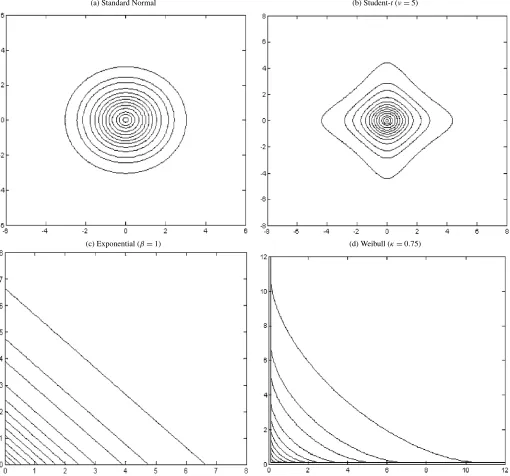
Note that the null should hold ask→ ∞. However, in prac-ticekis limited by the sample size. Thus, we chooseK suffi-ciently large so that we can handle relevant dependence struc-tures while keeping the theoretical framework tractable. In the following, we present the equations representing the boundaries of the autocontours, i.e., when the integral in Equation (2.3) holds with equality, corresponding to the most commonly en-countered densities in financial econometrics (seeAppendix A for details on construction of the autocontour equations for these densities):
In Figure1, we show the graphical contours corresponding to these cases.
2.2 Test Statistics and Asymptotic Distributions
For a given autocontourACRαi,k, we define a binary variable as follows ber of autocontours. Hence, this Bernoulli random variable
(a) Standard Normal (b) Student-t(ν=5)
(c) Exponential (β=1) (d) Weibull (κ=0.75)
Figure 1. Sample autocontours of bivariate distributions under independence.Notes: Autocontours are presented for the following coverage levels (%): 1, 5, 10, 20, 30, 40, 50, 60, 70, 80, 90, 95, and 99.
takes on value 1 if an observation falls outside the auto-contour and 0 otherwise. Note that this indicator can also be constructed the other way around, i.e., taking on value 1 if an observation falls inside the autocontour and 0 other-wise, producing the same set of results in a symmetric fash-ion. Since ACRαi,k contains αi% of observations, we ex-pect to have (1 −αi)% outside the autocontour. Let pi ≡ 1−αi. Under the null we have E[Itk,i] =pi and Var(Itk,i)= pi(1−pi). Furthermore, the indicator is a linearly dependent process with a moving average (MA) structure. Its autocovari-ance function is given by γhi =1(h =k)[P(Itk,i =1,Itk−,ih= 1)−p2i], i.e., there is dependence only at the kth lag. Our first test statistic is a t-statistic based on this indicator se-ries.
Proposition 1. Letpˆki = T−1kTt=−1kIkt,i. Under the null hy-pothesis given in Equation (2.4),
tk,i= √
T−k(pˆki −pi)
σk,i
d
→N(0,1),
whereσk2,i=pi(1−pi)+2γki.
Note thatpiis given under the null and a consistent estima-tor of the autocovariance term,γki, can be easily obtained from data. For a given autocontouri, we can examine the lag struc-ture of tk,i for k=1, . . . ,K and collect those t-statistics in a graph, which we callautocontourgram. See Section5for vari-ous empirical examples.
In the spirit of Box–Pierce–Ljung statistics, the information contained in the individualtk,i statistics can be pooled either
acrossKlags or acrossCcontours. The following two test sta-tistics consider the joint distribution oft-ratios associated with different lags or contours.
Proposition 2. For a given autocontouri, consider all lags up toK. Letqk,i=√T−k(pˆki −pi), k=1, . . . ,K, and stack
Proposition 3. For a given lagk, consider multiple contours. Let zi,k=
Since our testing framework imposes both implications of the null hypothesis, independence and correct density function, our statistics have power against violations of both. As an example, consider the case where the null assumes thatεt is iid normal, but in reality there is neglected dependence in the conditional mean. Under the alternative, we have elliptical autocontours as opposed to circles implied by the null. Now suppose the null assumes iid normal innovations, butεtis in fact an independent Student-tprocess. The actual autocontours will look like Fig-ure1(b), whereas the null implies circles as in Figure1(a). The discrepancy between the autocontours in these cases is what makes our tests powerful in detecting departures from the null in either direction. Whenever there is neglected dependence, t andJ-statistics will exhibit particular patterns signaling the form of the violation, e.g., significance at early lags, but a fast decay in case of linear dependence. Similar arguments apply to theQ-statistics. When the null is rejected because of an in-correctly assumed density function, the t andJ-statistics will be significant, but they will not display any specific dynamic patterns. Finally, when the rejection comes from violations of both dependence and the density function, it will be desirable to combine our omnibus tests with tests that are powerful against violations of the null in a single direction, e.g., Escanciano (2008),Fernandes and Grammig(2005), andHong(1996).
3. PARAMETER UNCERTAINTY
Even though the tests we propose can be applied to raw data, they will be most useful as a diagnostic tool for model specifi-cation. Thus, in practice we will be analyzing residuals,εˆt(θˆT), which depend on parameter estimates, instead of the true error εt(θ0). Our tests are subject to the uncertainty created by pa-rameter estimation. The following discussion will be centered around thet-statistics,tk,i, considered in Proposition1, but the same conclusions will apply to the QKi and JkC tests given in Propositions2and3, respectively.
To understand how parameter estimation affects the tests, let us take a mean value expansion and apply Slutsky’s Theorem, e.g.,Randles(1982). This yields cally equivalent. We make the following assumptions to obtain the asymptotic distribution under parameter uncertainty:
A1. √T(θˆT − θ0) →d N(0,A−1BA−1) where A ≡ Hessian matrix and the score vector corresponding to quasi-maximum likelihood (QML) estimation. A1 is based on standard quasi-maximum likelihood estimate (QMLE) arguments. A2 guarantees that the gradient vector is bounded. A3 is a weak assumption that is required to have a well-defined asymptotic variance. A2 and A3 can be straight-forwardly verified for commonly used models.
Proposition 4. Under A1–A3 we have √
T(pˆki(θˆT)−pi)→d N(0, τ2 k,i),
where τk2,i=σk2,i+D′A−1BA−1D+2E[√T(pˆik(θˆT)−pi)× S′(θ0)]A−1D.
Proposition 5. For a Gaussian location-scale model yt = μ0+σ0εt, whereεt∼iid N(0,1), we have
wherefzt is the pdf ofzt, a chi-squared random variable with 2 degrees of freedom.
This proposition states that the estimation of the parameters in the mean does not affect the asymptotic distribution of the test (D1=0) for the case when the variance is known. This result also holds for a model with Student-tinnovations.
In general, it will be difficult to obtain an empirical counter-part of the gradient vectorD. In addition, for some models the covariance terms given in A3 may be difficult to estimate, e.g., simulation-based methods reviewed in Gouriéroux and Mon-fort(1996). Therefore, we propose to estimate the asymptotic varianceτk2,iusing a bootstrap procedure. This is a commonly used approach in the literature to overcome the difficulties asso-ciated with asymptotic variance estimation in various contexts (seeEfron 1979;Buchinsky 1995; andLedoit, Santa-Clara, and Wolf 2003among others). The bootstrap estimator of the vari-ance in Proposition 4 is given by
ˆ parameter estimate from thebth bootstrap sample. For the chi-squared statistics, the covariance matrix estimators are defined analogously. We prefer a parametric bootstrap since the null hy-pothesis fully specifies the parametric data generating process (DGP) (seeHorowitz 2001). In particular, bootstrap samples are obtained from Equation (2.1) by replacingθ0withθˆT and gen-eratingεtfrom the specified parametric distribution. Under suit-able regularity conditions, this estimator should be consistent as proven within the linear regression context for iid observations byLiu and Singh(1992), and for dependent data byGoncalves and White(2005). Alternatively, one can bootstrap the full dis-tribution of the test statistics. However, our test statistics are not asymptotically pivotal under parameter uncertainty, and this im-plies that the bootstrap distribution does not necessarily provide a superior approximation to the finite sample distributions of test statistics, seeHorowitz(2001). Monte Carlo results (to be presented in the following section) indicate that bootstrapping the asymptotic covariance matrices and using standard asymp-totic critical values delivers remarkable results in terms of size and power of the tests.
4. MONTE CARLO SIMULATIONS
4.1 Size of the Tests
For size simulations we consider the following three cases: 1. yt=μ+σ εt,εt∼iid N(0,1),μ=1.25, andσ=2. 2. yt=μ+σ εt√(ν−2)/ν,εt∼iid Student-t(ν),μ=1.25,
σ=2, andν=5.
3. yt=σ εt,εt∼iid exp(β),σ=2, andβ=1.
The Gauss 7.0 random number generator is used to generate pseudo random numbers from the three distributions. We apply the tests to the properly standardized residuals,εˆt≡(yt− ˆμ)/σˆ. Because of computational considerations, the number of Monte Carlo replications is 1000. The number of bootstrap replications is 500. We consider 13 autocontours(C=13)with coverage levels (%): 1, 5, 10, 20, 30, 40, 50, 60, 70, 80, 90, 95, and 99, spanning the entire density function. The nominal size level is 5%.
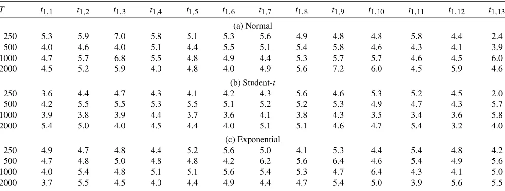
In Table1we report the results fort1,i,i=1, . . . ,13. There are no systematic deviations from the nominal size either across autocontours or across distributions with some exceptions for the 1% and 99% autocontours whenT=250. This result is not surprising because in small samples there is not enough varia-tion at the extreme contours (1% and 99% coverage).
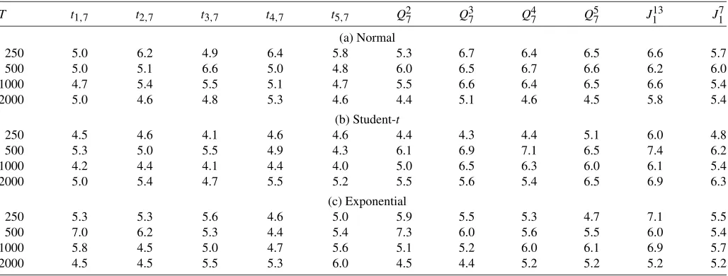
To check the size robustness of thet-statistics for different lags, we exclusively focus on the 50% autocontour(i=7)and considerk=1, . . . ,5. We report these results in Table2. Over-all the simulated size values are around 5% indicating good size for all distributions. These results are robust across all the auto-contours and also available from the authors upon request. We also report the size results for theQ-statistic(QK7,K=2, . . . ,5) and theJ-statistic (J113 andJ17), respectively, in Table2. Over-all,Q-statistics have acceptable size. For theJ-statistic, when we consider all 13 autocontours, there is a tendency for the test to over-reject, but when we focus on the middle autocontours by removing the first three (1%, 5%, and 10%) and the last three (90%, 95%, and 99%), the empirical size improves sub-stantially, approaching the nominal size even for small samples.
Table 1. Size of thet-statistics
T t1,1 t1,2 t1,3 t1,4 t1,5 t1,6 t1,7 t1,8 t1,9 t1,10 t1,11 t1,12 t1,13
(3)yt=1.25εt,εt∼iid exp(1). Number of Monte Carlo replications: 1000; bootstrap replications: 500; nominal size: 5%.
Table 2. Size of thet, Q, andJ-statistics
T t1,7 t2,7 t3,7 t4,7 t5,7 Q27 Q37 Q74 Q57 J113 J17
(a) Normal
250 5.0 6.2 4.9 6.4 5.8 5.3 6.7 6.4 6.5 6.6 5.7
500 5.0 5.1 6.6 5.0 4.8 6.0 6.5 6.7 6.6 6.2 6.0
1000 4.7 5.4 5.5 5.1 4.7 5.5 6.6 6.4 6.5 6.6 5.4
2000 5.0 4.6 4.8 5.3 4.6 4.4 5.1 4.6 4.5 5.8 5.4
(b) Student-t
250 4.5 4.6 4.1 4.6 4.6 4.4 4.3 4.4 5.1 6.0 4.8
500 5.3 5.0 5.5 4.9 4.3 6.1 6.9 7.1 6.5 7.4 6.2
1000 4.2 4.4 4.1 4.4 4.0 5.0 6.5 6.3 6.0 6.1 5.4
2000 5.0 5.4 4.7 5.5 5.2 5.5 5.6 5.4 6.5 6.9 6.3
(c) Exponential
250 5.3 5.3 5.6 4.6 5.0 5.9 5.5 5.3 4.7 7.1 5.5
500 7.0 6.2 5.3 4.4 5.4 7.3 6.0 5.6 5.5 6.0 5.4
1000 5.8 4.5 5.0 4.7 5.6 5.1 5.2 6.0 6.1 6.9 5.7
2000 4.5 4.5 5.5 5.3 6.0 4.5 4.4 5.2 5.2 5.2 5.2
NOTE: Simulated size oft,Q, andJ-statistics for three DGPs (see the notes to Table1for details).
From a practical point of view, one may not want to use auto-contours too small or too large when the sample size is small.
4.2 Power and Consistency of the Tests
To analyze the power properties of our test statistics we con-sider three alternative data generating processes and apply our tests to the standardized residuals generated by the estimation of the following location-scale models, where μ=1.25 and σ=2 in all cases:
1. yt=μ+σ εt,εt=φεt−1+utwhereut∼iid N(0,1−φ2). 2. yt=μ+σ εt√(ν−2)/ν, whereεt∼iid Student-t(ν). 3. yt=μ+σ εt, εt=√htut whereut∼iid N(0,1), ht =
ω+αε2t−1+βht−1.
For all three cases the null hypothesis is εt ∼iid N(0,1). In case 1 we investigate departures from the independence hy-pothesis by considering different values of the autoregressive parameter, φ∈ {0.5,0.9}. In case 2, we maintain the inde-pendence hypothesis and investigate departures from the hy-pothesized density functional form by generating iid data from the Student-t distribution for two different values of the shape parameter, ν ∈ {5,15}. The variance is normalized to unity to control for the scale effects. Finally, in case 3 we ana-lyze departures from both dependence and functional form by generating data from a generalized autoregressive condi-tional heteroscedasticity (GARCH)(1, 1) model with(α, β)∈ {(0.05,0.9), (0.15,0.8)}. We setω=1−α−β to normalize the unconditional variance to 1.
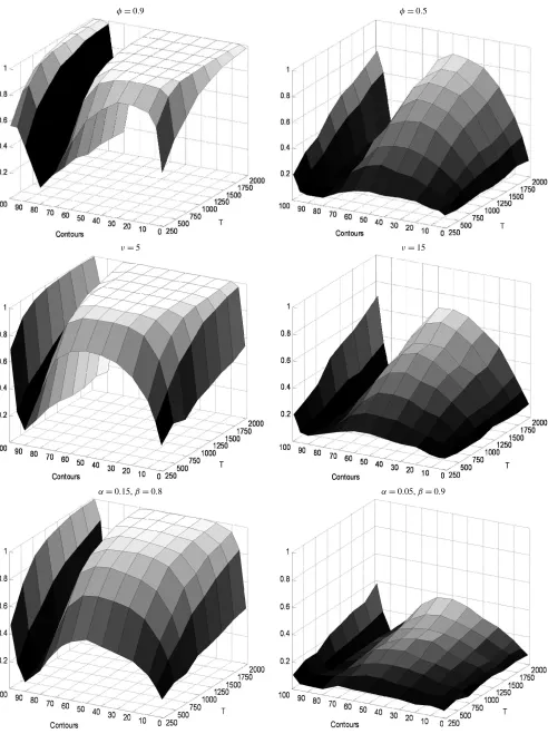
In Figure 2, we present the power surfaces for t1,i, i = 1, . . . ,13, for samples sizes ranging from 250 to 2000 observa-tions and for the 13 autocontours. In the autoregressive case 1, the power of thet-statistics approaches 1 rather quickly for high values of the autoregressive parameter, though there is a sub-stantial drop in power for autocontours around the 80% cover-age level. In the Student-tcase 2, the power approaches 1 very quickly for low degrees of freedom. For instance, in the 99% autocontour, the power is as high as in the central autocontours
for all sample sizes due to the leptokurtosis of the Student-t den-sity. As anticipated, rejection rates decrease asνgets larger, for which the null and the alternative become less distinguishable. The power surface exhibits the lowest values at the 90% auto-contour, for which the null and the alternative hypotheses are very close to each other. In the GARCH case 3, the data are un-correlated but dependent through the second moments. There is also excess kurtosis relative to the normal distribution. Persis-tence is the same across the two alternative parameterizations (α+β=0.95), but kurtosis and the level of first order auto-correlation in the second moment is increasing withα. As ex-pected, the power of the test is increasing inα. Whenα=0.05, the excess kurtosis in the data is only 0.16 and the first order autocorrelation in the second moment is only 0.0725, so the de-parture from the null is fairly weak.
The substantial drop in power at particular coverage levels observed in Figure2should not be interpreted as a lack of con-sistency of the t-test, but rather as the difficulty of any test to discriminate between a null and an alternative hypothesis that are very close to each other for a fixed sample size. To un-derstand why, let us focus on case 2 since the same reasoning will apply to the others. Let η≡1/ν, so that under normal-ityH0:η=0, and under Student-t H1:η >0. The asymptotic power of thet-test, sayT(η), for a fixed contouriand a fixed lagkat theα-significance level is given by:
T(η) = P √
T|ˆpki −pi(η)|
≥σk,i(0)z1−α/2− √
T|pi(η)−pi(0)|
→1− σ
k,i(0)z1−α/2−√T|pi(η)−pi(0)| σk,i(η)
+
σ
k,i(0)zα/2− √
T|pi(η)−pi(0)| σk,i(η)
.
We can see that the power will increase whenever pi(η)= pi(0), and it will be equal to the size wheneverpi(η)=pi(0). Thus, if the null and the alternative hypothesis are very close to each other we will need a substantial number of obser-vations for √T|pi(η)−pi(0)| not to vanish. In Table 3 we
φ=0.9 φ=0.5
ν=5 ν=15
α=0.15,β=0.8 α=0.05,β=0.9
Figure 2. Power of thet-statistics.Notes: Simulated power of thet-statistic for all 13 autocontours and the first lag(k=1)under the following DGPs: (1)yt=1.25+2εt,εt=φεt−1+ut,ut∼iid N(0,1−φ2); (2)yt=1.25+2εt√(ν−2)/ν,εt∼iid Student-t(ν); and (3)yt=1.25+2εt,
εt=√htut, whereut∼iid N(0,1),ht=ω+αε2t−1+βht−1.The null hypothesis isεt∼iid N(0,1). All test statistics are based on standardized
residuals. Number of Monte Carlo replications: 1000; number of bootstrap replications: 500; nominal size: 5%.
Table 3. Difference in violation percentages between Normal and Student-t
pi(η)−pi(0)
i ν=5 ν=10 ν=15
1 −0.0050 −0.0019 −0.0011 2 −0.0236 −0.0089 −0.0055 3 −0.0436 −0.0167 −0.0103 4 −0.0735 −0.0289 −0.0180 5 −0.0911 −0.0368 −0.0230 6 −0.0974 −0.0403 −0.0254 7 −0.0937 −0.0395 −0.0250 8 −0.0809 −0.0344 −0.0218 9 −0.0602 −0.0253 −0.0160 10 −0.0329 −0.0125 −0.0076 11 −0.0017 0.0025 0.0023 12 0.0127 0.0092 0.0066 13 0.0174 0.0095 0.0063
NOTE: pi(η)is the theoretical violation percentage under the alternative hypothesis.
η=1/ν, whereνdenotes degrees of freedom of the Student-tdistribution.pi(0)is the
theoretical violation percentage under the null hypothesis of normality. The true distribu-tion is Student-twith degrees of freedom equal toν.
show the difference pi(η)−pi(0)for ν=5,10,15. It is ex-actly for the 90% autocontour that the difference is the small-est, by as much as one order of magnitude, e.g., for ν=5, pi(η)−pi(0)= −0.0017. To provide further insight, we repli-cated the same simulation as in Figure2forν=5 and for the 90% autocontour(i=11)with sample sizes larger than 2000 observations. We find that a substantial number of observations will be needed to discriminate the null and the alternative hy-potheses (more than 125,000 for a rejection rate above 60%), but eventually the power will approach 1 so that the test is con-sistent.
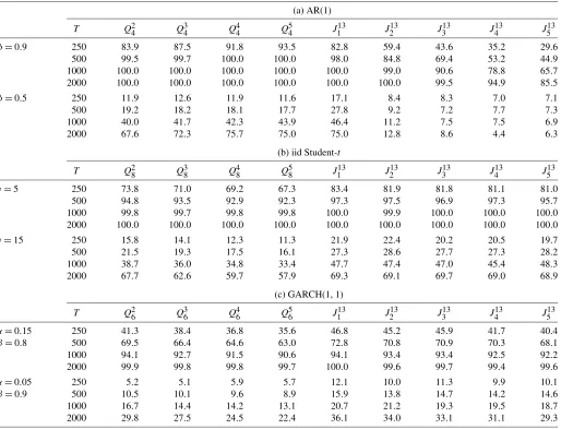
In Table 4, we report the power of the Qand J-statistics. ForQ-statistics we present power results for a different auto-contour in each case to offer a comprehensive analysis. In all three cases the rejection rates are high and behave in the right direction. The power is close to 1 for samples larger than 500 when there is high dependence, or a large departure from nor-mality. When the dependence is due to strong autoregressive conditional heteroscedasticity (ARCH) effects, a sample size of 500 provides reasonable power. In case 1 when the depen-dence is high we observe an increase in rejection rates as K increases. This is expected given the sensitivity of the test to lin-ear dependence. On the other hand, we do not observe a similar
Table 4. Power of theQandJ-statistics
(a) AR(1)
T Q24 Q34 Q44 Q54 J131 J132 J133 J134 J135 φ=0.9 250 83.9 87.5 91.8 93.5 82.8 59.4 43.6 35.2 29.6
500 99.5 99.7 100.0 100.0 98.0 84.8 69.4 53.2 44.9 1000 100.0 100.0 100.0 100.0 100.0 99.0 90.6 78.8 65.7 2000 100.0 100.0 100.0 100.0 100.0 100.0 99.5 94.9 85.5
φ=0.5 250 11.9 12.6 11.9 11.6 17.1 8.4 8.3 7.0 7.1 500 19.2 18.2 18.1 17.7 27.8 9.2 7.2 7.7 7.3 1000 40.0 41.7 42.3 43.9 46.4 11.2 7.5 7.5 6.9 2000 67.6 72.3 75.7 75.0 75.0 12.8 8.6 4.4 6.3
(b) iid Student-t
T Q28 Q38 Q48 Q58 J131 J132 J133 J134 J135 ν=5 250 73.8 71.0 69.2 67.3 83.4 81.9 81.8 81.1 81.0
500 94.8 93.5 92.9 92.3 97.3 97.5 96.9 97.3 95.7 1000 99.8 99.7 99.8 99.8 100.0 99.9 100.0 100.0 100.0 2000 100.0 100.0 100.0 100.0 100.0 100.0 100.0 100.0 100.0
ν=15 250 15.8 14.1 12.3 11.3 21.9 22.4 20.2 20.5 19.7 500 21.5 19.3 17.5 16.1 27.3 28.6 27.7 27.3 28.2 1000 38.7 36.0 34.8 33.4 47.7 47.4 47.0 45.4 48.3 2000 67.7 62.6 59.7 57.9 69.3 69.1 69.7 69.0 68.9
(c) GARCH(1, 1)
T Q26 Q36 Q46 Q56 J131 J132 J133 J134 J135 α=0.15 250 41.3 38.4 36.8 35.6 46.8 45.2 45.9 41.7 40.4 β=0.8 500 69.5 66.4 64.6 63.0 72.8 70.8 70.9 70.3 68.1 1000 94.1 92.7 91.5 90.6 94.1 93.4 93.4 92.5 92.2 2000 99.9 99.8 99.8 99.7 100.0 99.6 99.7 99.4 99.6
α=0.05 250 5.2 5.1 5.9 5.7 12.1 10.0 11.3 9.9 10.1 β=0.9 500 10.5 10.1 9.6 8.9 15.9 13.8 14.7 14.2 14.6 1000 16.7 14.4 14.2 13.1 20.7 21.2 19.3 19.5 18.7 2000 29.8 27.5 24.5 22.4 36.1 34.0 33.1 31.1 29.3
NOTE: Simulated power of theQandJ-statistics under three DGPs (see the notes to Figure2for details).
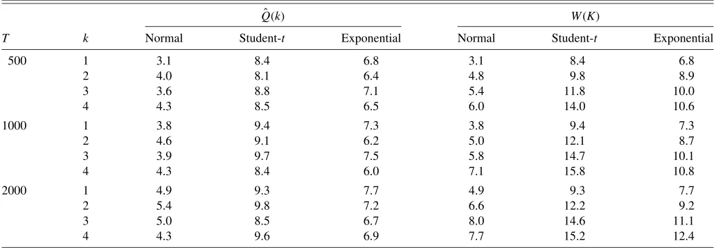
Table 5. Size simulations for Hong–Li tests
ˆ
Q(k) W(K)
T k Normal Student-t Exponential Normal Student-t Exponential
500 1 3.1 8.4 6.8 3.1 8.4 6.8
2 4.0 8.1 6.4 4.8 9.8 8.9
3 3.6 8.8 7.1 5.4 11.8 10.0
4 4.3 8.5 6.5 6.0 14.0 10.6
1000 1 3.8 9.4 7.3 3.8 9.4 7.3
2 4.6 9.1 6.2 5.0 12.1 8.7
3 3.9 9.7 7.5 5.8 14.7 10.1
4 4.3 8.4 6.0 7.1 15.8 10.8
2000 1 4.9 9.3 7.7 4.9 9.3 7.7
2 5.4 9.8 7.2 6.6 12.2 9.2
3 5.0 8.5 6.7 8.0 14.6 11.1
4 4.3 9.6 6.9 7.7 15.2 12.4
NOTE: Simulated size (%) of theQandW-statistics ofHong and Li(2005) for three DGPs (see the notes to Table1for details). Nominal size is 5%.
pattern in the GARCH(1,1)case where the dependence comes through higher moments. Regarding theJ-statistic, a common characteristic across all three DGPs is that for a given sample size the power is roughly the same as the maximum power of thet-statistics. The pattern on rejection frequencies is the same as that of the individual t-statistics. In case 1, the rejection is stronger when there is high dependence even for small samples. There is a decrease in power askincreases, which is more evi-dent when the autoregressive parameter is small. This is some-how expected because the DGP is only an AR(1)process. In case 2, the test is more powerful for small degrees of freedom, but we should mention that even forν=15 the power of the test is still high, around 69% for 2000 observations. In case 3, we have stronger rejections rates when the data exhibit higher levels of kurtosis and stronger autocorrelation in the second mo-ment.
4.3 Comparison of the Autocontour Tests With Hong and Li’s Tests
We offer a comparison of our tests with the most recent tests proposed by Hong and Li (2005), who entertained the same joint null hypothesis of iid-ness and density functional form as that of our autocontour tests. There are other para-metric and nonparapara-metric tests, like those in Engle and Rus-sell (1998), Fernandes and Grammig (2005), and Meitz and Terasvirta(2006), among others, that focus on a single hypoth-esis, either dynamic specification or density functional form. Thus, by focusing on a test with the same joint hypothesis we will be able to provide a fair comparison. Moreover, since Hong and Li’s test is nonparametric in nature, our comparison will provide an assessment of the advantages of a parametric test versus a kernel-based nonparametric test.
Hong and Li’s tests are based onut=Ft(yt|ℑt−1;θ0), which must be iid U[0,1]under correct specification. The test has a null hypothesis of iid U[0,1]and it compares the estimate of the joint density of {ut,ut−j}with the product of two U[0,1] densities, which is equal to 1. They propose two tests: (i) for a given displacement k, Qˆ(k)→d N(0,1), and (ii) W(K)= K−1/2Kk=1Qˆ(k)→d N(0,1). Thus, the Qˆ(k)test is similar to
our autocontour tests with a fixed displacementk, such astk,i andJCk, and theW(K)is similar to the autocontour testQKi that aggregates over displacements.
We ran the same set of Monte Carlo experiments described previously with the Hong and Li (2003) tests. The results con-cerning the size of the tests are displayed in Table 5, which are directly comparable with those for our tests reported in Ta-ble2. The autocontour tests,tk,iandQKi , and the HL tests,Qˆ(k) andW(K), have a similar size in testing for independence and normality. The main difference arises in testing for Student-t and Exponential distributions. In both instances, the HL tests are heavily oversized. In particular, theW(K) test has a size more than twice the nominal size in the Student-tand Exponen-tial cases. These distortions in size are typical in nonparametric kernel-based tests.
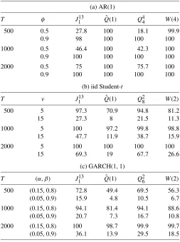
On the power front, the autocontour tests are substantially more powerful in detecting deviations from the density func-tional form and dependence in higher moments. The HL tests have more power in detecting linear dependence. The simula-tion results on power differences are displayed in Table6. The null hypothesis isεt∼iid N(0,1). Since the size of the HL tests are reasonable for this null hypothesis we use their asymptotic distribution to assess the power properties. Since we already use the asymptotic distributions of the autocontour tests, both tests are compared on equal grounds. As a side note, an assess-ment of the power of the HL tests under nonnormal densities will require a size correction through resampling techniques.
In the Gaussian AR(1) case, the HL tests are very power-ful even for small autoregressive parameters and small sample sizes. For high levels of dependence both tests are very similar. In the iid Student-tcase, the autocontour tests dominate across degrees of freedom and sample sizes. For instance, a Student-t with 15 degrees of freedom is relatively close to a normal den-sity, yet the autocontour tests have power of about 69% ver-sus the HL tests, which have rejection rates around 20%. In the third case, where the DGP is a GARCH(1,1)process, the au-tocontour tests are more powerful throughout. As we saw in the previous simulations, the power decreases when theα pa-rameter is small, but even in this case our tests have more than twice the power of the HL tests. Overall, our assessment is that the autocontour tests have considerable advantages over the HL
Table 6. Power comparison of autocontour and Hong–Li tests
NOTE: Simulated power (%) of the autocontourJandQ-statistic versusQˆandWtests of Hong–Li for three DGPs (see the notes to Figure2). The null hypothesis isεt∼iid
N(0,1).
tests as they offer a very good size and high power in almost all instances considered.
5. EMPIRICAL APPLICATION
Our application is concerned with dynamic specification and density functional form in autoregressive conditional duration (ACD) models for trade duration data.Bauwens et al.(2004) andFernandes and Grammig(2005), among others, called our attention to a void in the literature on duration models, which despite being extremely popular in recent years, have not re-ceived much attention in what concerns the testing for model specification. Thus,Bauwens et al.(2004) proposed the eval-uation of the density forecast in the manner ofDiebold, Gun-ther, and Tay(1998) as a test on the distributional specification of several ACD models. Fernandes and Grammig proposed a nonparametric procedure to test the specification of the density in ACD models assuming that the conditional mean process is correctly specified. We aim to contribute to this literature by ap-plying our autocontour tests to ACD models. Our contribution brings different aspects to the testing question. Bauwens et al. did not take into account parameter uncertainty and Fernandes and Grammig’s approach is nonparametric while our approach takes parameter uncertainty into account; it is parametric and it does not presume that the conditional mean duration is cor-rectly specified. In this sense, our tests may point pitfalls of the model in both directions (mean and density) versus just one.
We consider an ACD model for trade durations (time inter-vals between transactions) of the Airgas common stock from March 1 to December 31, 2001 with a total of 32,366 obser-vations. Let t1,t2, . . . ,ti, . . . denote a sequence of transaction times, then durations are defined as xi=tt−ti−1.Engle and Russell(1998) introduced the ACD model for durations, which is given by, model with quasi-maximum likelihood under exponential den-sity. Through a battery of standard tests, Engle and Russell (2009) pointed out that this specification is successful in cap-turing the time dependence in durations. With the autocontour tests we aim to analyze the advantages and disadvantages of the three most popular distributional assumptions onεi: (i) Expo-nential, (ii) Weibull, and (iii) Burr. For Weibull and Burr dis-tributions, we need to conduct a second step to obtain the es-timates of the shape parameters. The eses-timates are κˆ =0.75 under Weibull andγˆ=0.05 andκˆ=0.77 under Burr. The Burr density reduces to Weibull whenγ =0, thus the parameter es-timates suggest that the distributions are empirically close to each other.
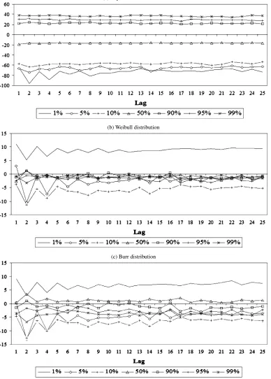
We restrict our discussion to the t and J-statistics to save space. We summarize the results in Figures3 and4. The ex-ponential distribution is overwhelmingly rejected for all cover-age levels. Figure3(a) shows that rejection is the strongest in the lower and the tail contours. For small coverage levels (1%, 5%, and 10%), the exponential density leaves too few obser-vations outside the autocontours (negativet-statistics), thus we need a different density that squeezes the contours inward. On the contrary, for large coverage levels (90%, 95%, and 99%) the exponential leaves too many observations outside the auto-contour (positivet-statistics). This means that exponential dis-tribution is not putting enough probability mass on large du-rations. The Weibull density corrects these distortions to some extent. In Figure3(b) we see that the Weibull distribution does a good job of assigning higher probabilities to large durations so that the tests at the 90%, 95%, and 99% autocontours are not statistically significant at conventional confidence levels. However, Weibull overcorrects the probability mass of the very small durations as the 1% autocontourt-test changes signs from negative [Figure 3(a)] to positive [Figure3(b)], but it cannot place enough probability on just small durations, those within the 5% and 10% autoncontours (the t-statistics are still nega-tive). Sinceκ <ˆ 1 the Weibull autocontours have asymptotes, implying that extremely small durations can have substantial probability mass, in fact more than empirically justifiable. This finding on Weibull is in agreement with that ofBauwens et al. (2004) where a different dataset was analyzed. However, we re-ject the exponential distribution because it does not put enough mass on the very small durations, whereas in Bauwens et al. the exponential is rejected for the opposite reason. Furthermore, they argued that the exponential assumption is adequate for the
(a) Exponential distribution
(b) Weibull distribution
(c) Burr distribution
Figure 3. t-Statistics for ACD(3,2)model of Airgas transaction durations.Notes:t-statistic for selected autocontours for the residuals of the exponential, Weibull, and Burr distributions ACD(3,2)models fitted to Airgas trade durations. Statistics outside the[−1.96,1.96]range are significant at 5% level.
tail while we strongly reject this in our analysis. The perfor-mance of the Burr distribution is similar to that of Weibull for small and very small autocontours. However, unlike Weibull, Burr overcorrects the tails and the tests keep on rejecting Burr with respect to both 95% and 99% autocontours [Figure3(c)].
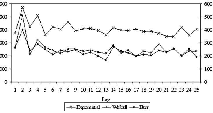
TheJ-statistics, which aggregate information from all auto-contours, are plotted in Figure4. It is clear that all three
distri-butions are rejected by the data even though Weibull and Burr provide a clear improvement over Exponential. This pessimistic view is also shared byBauwens et al.(2004). However, these results give a direction to search for new densities. The Weibull is a good starting point because it attaches the right probability mass to the tails (very large durations) and to durations within the middle contours, but it needs some corrections for the very
Figure 4. J-statistics for ACD(3,2)model of Airgas transaction durations.Notes:J-statistic based on all 13 autocontours for the residuals of the Exponential (left-scale), Weibull, and Burr (right-scale) ACD(3,2)models fitted to Airgas trade durations. 5% critical value is 22.3.
small and small durations. These adjustments can be made non-parametrically so that the proposed density enjoys a parametric and a nonparametric component.
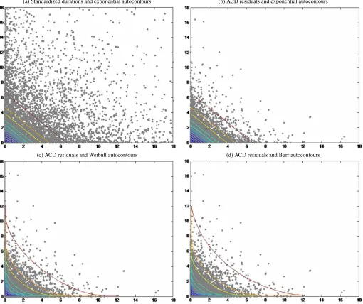
It is illustrative to look at a scatterplot of the data together with the autocontours under various distributional assumptions. In Figure 5 we show a subset of the data (first 7500 obser-vations). In Figure5(a), we plot the raw durations divided by the sample mean. This is the case where dynamics are ignored and an iid exponential assumption is imposed. In Figures5(b) through (d) we plot the ACD(3,2)residuals under Exponen-tial, Weibull, and Burr distributions. In these three panels we can observe the success of the ACD model in capturing the du-ration dynamics and the failure of the exponential distribution to capture mainly the probability of very small and large dura-tions. Figure5(c) shows that Weibull provides a great improve-ment over Exponential. By transforming the boundaries of the autocontours from straight lines to curves bended toward the origin, Weibull assigns relatively more probability mass to both small and large durations. However, because of the autocontour asymptotes, it assigns unnecessarily large probabilities to very small durations and leaves out too many observations outside the 1% autocontour. Figure5(d) clearly illustrates the failure of Burr to improve over Weibull, mainly when large durations are concerned.
6. CONCLUSION
The methodological advances in two fronts of time series analysis—nonlinear models with nonnormal density functions, and density forecasting—emphasized the need for developing dynamic specification tests for the joint hypothesis of iid-ness and density functional form. In this article we propose a new battery of tests that rely on the fundamental properties of in-dependent random variables with identical distributions and we introduce a graphical device, theautocontour. We believe that our approach brings considerable advantages over existing methods. Our tests are very powerful against violations of both hypotheses, iid-ness, and density function; they have parametric
convergence rates and standard limiting distributions; and they take into account the uncertainty introduced by parameter esti-mation. A comparison with Hong and Li’s tests, which are non-parametric, shows that the autocontour tests are more powerful to detect nonlinear dependence and deviations from the hypoth-esized density function. We applied our tests to ACD models and conclude that none of the conditional densities assumed in the literature provides a good fit to model trade durations. Con-trary to the standard findings in returns data, where the problem is the leptokurtosis generated by very large returns, in duration data the problem lies on the probability assigned to very small durations, which is substantially more (Weibull/Burr densities) or substantially less (Exponential density) than empirically is justifiable.
While we introduced our methodology within the context of pair-wise independence, it can also be extended to higher di-mensions. On going further than the bivariate case we will be losing the graphical representation of the autocontour, which is helpful for understanding the modeling problem; however, once the analytical functional form of the autocontour is obtained, the indicator variable is easy to construct and the proposedt -tests and chi-squared -tests will follow naturally.
APPENDIX A: CONSTRUCTION OF THE AUTOCONTOURS
In case of standard normal distribution the joint density of interest is given by
f(εt, εt−k)= 1 2π exp
−1
2(ε 2 t +ε
2 t−k)
. (A.1)
For a fixed value of this density, sayfα, we haveε2t +ε2t−k=aα
whereaα= −2 ln(2πfα). Thus, autocontours are circles with
radius√aα, which can be computed by numerical integration
using the following equation,
√aα
−√aα
g(εt) −g(εt)
f(εt, εt−k)dεtdεt−k=α, (A.2)
(a) Standardized durations and exponential autocontours (b) ACD residuals and exponential autocontours
(c) ACD residuals and Weibull autocontours (d) ACD residuals and Burr autocontours
Figure 5. Data and autocontours under different distributions.Notes: Panel (a) presents the results for durations standardized by the sample mean. Panels (b), (c), and (d) are based on ACD(3,2)residuals.εtis on the vertical axis andεt−1is on the horizontal axis. A color version of
this figure is available in the electronic version of this article.
whereg(εt)=
aα−ε2t. Alternatively, one can get thea val-ues based on the cdf of a chi-squared random variable with 2 de-grees of freedom due to the normality assumption, e.g., for 90% autocontoura0.9=4.61.
In case of Student-tand exponential distributions the value ofaαcan be computed by numerical integration along the lines
illustrated previously. For Weibull and Burr distributions, the autocontours cannot be easily derived by integration, so we need to resort to simulation methods. Further details on both techniques can be found in the Supplemental Appendix.
APPENDIX B: MATHEMATICAL PROOFS
Please note that some of the following proofs are presented in a compact form to save space. The interested reader is referred to the Supplemental Appendix for a complete exposition.
Proof of Proposition1
The result directly follows from the central limit theorem for covariance stationary processes presented inAnderson(1971).
Proof of Proposition2
Without loss of generality, let us consider the joint distribu-tion ofqk,iandql,i. Letx≡λ1qk,i+λ2ql,iwhereλ1andλ2are arbitrary constants and assumek<l. Then
x=λ1 √
T−k(pˆki −pi)+λ2 √
T−l(pˆli−pi).
Since all results are asymptotic we drop the first(l−k) obser-vations onItk,ito use the same scaling factor. Then we have
x=√1 T−l
T−l
t=1
[λ1(Ikt,i−pi)+λ2(Itl,i−pi)].
Defineet=λ1(Itk,i−pi)+λ2(Itl,i−pi), thenx=√T1−lTt=−1let. The first two moments ofetand its autocovariance function are given by theorem (CLT) for covariance stationary processes,x→d N(0, σx2)whereσx2=Var(et)+2 Cov(et,et−k)+2 Cov(et,et−l)+ 2 Cov(et,et−l+k). Thus, we show that any linear combination ofqk,iandql,iis asymptotically normal, establishing their joint asymptotic normality.
Now let us focus on the elements of the asymptotic co-variance matrix. Given that E[qk,i] =E[ql,i] =0, we have proof of Proposition2andxcan be shown to be asymptotically normal. Similar reasoning applies to the elements of the covari-ance matrix.
Proof of Proposition4
From assumption A1 in the main text we have, √ ing the argument of the score we obtain,
x=√1
Assumptions A2 and A3 guarantee finiteness of the vari-ance and covarivari-ance terms. Applying the CLT, we have x→d N(0, σx2)whereσx2=Var(et)+2 Cov(et,et−k). The variables on the right-hand side of Equation (3.1) are both asymptot-ically normal due to Proposition 1 and assumption A1. We just showed asymptotic normality of their linear combinations, which completes the proof.
Proof of Proposition5
Letθ0=(μ0, σ02)′. In this case the indicator series is con-structed as follows Ikt,i(zt(θ0))=(zt(θ0)−aαi >0), where
zt(θ0)=ε2t(θ0)+ε2t−k(θ0). From the mean value expansion in the text we need the following:
V12≡ lim
From the properties of the QML estimator
V12=CovItk,i(zt(θ0)),s′t(θ0)
+CovItk,i(zt(θ0)),s′t−k(θ0)+o(1).
For the model under consideration, we haves′t=(εt/σ0, (εt2− 1)/2σ02). Hence, we need to obtain (i)E[Itk,iεt], (ii)E[Itk,iεt−k], (iii)E[Itk,iε2t], and (iv)E[Ikt,iεt2−k]to get the covariance term. It can be shown that (i) and (ii) are both zero and (iii) and (iv) are given by 1−√aαi
whereδ(x)is the Dirac delta function (seeArfken 2005for fur-ther details on Dirac delta function andPhillips 1991for a sim-ilar application). To simplifyD1andD2, we use the following properties of the Dirac delta function:
δ(x−a)=0 forx=a, (B.5) where a is a finite constant and h is any continuous func-tion. Using Equations (B.5) through (B.7), we can show that D1=0. Applying Equation (B.6) directly to Equation (B.4) yieldsE[δ(zt−aαi)zt] =aαifzt(aαi), which completes the proof.
SUPPLEMENTAL MATERIALS
Supplemental Appendix: This document contains an extend-ed literature survey, additional Monte Carlo simulation re-sults, and a more detailed exposition of some of the mathe-matical proofs. (Autocontour_Supp_Apdx.pdf)
ACKNOWLEDGMENTS
The authors thank Yongmiao Hong and Haitao Li for provid-ing the computer code for their test procedure and Jeff Russell for providing us with the duration dataset. We would also like to thank the participants in the 2006 NBER/NSF Time Series Conference in Montreal, the 2006 International Symposium in Forecasting in Santander (Spain), the 2007 Far-Eastern Meet-ings of the Econometric Society in Taipei (Taiwan), the 2007 (EC)2 Conference in Faro (Portugal), and the 2008 Sympo-sium of the SNDE in San Francisco for their comments and insights. Special thanks to Aman Ullah, Tae-Hwy Lee, and Christian Bontemps. We are also grateful to the editor, Arthur Lewbel, associate editor, and two anonymous referees whose constructive comments have greatly improved this manuscript. The usual caveat applies. The first author appreciates financial support from the UCR Academic Senate grants and the Univer-sity Scholar award.
[Received May 2008. Revised October 2009.]
REFERENCES
Anderson, T. W. (1971),The Statistical Analysis of Time Series, New York: Wiley. [198]
Andrews, D. W. K. (1997), “A Conditional Kolmogorov Test,”Econometrica, 65, 1097–1128. [186]
Arfken, G. B. (2005),Mathematical Methods for Physicists, Amsterdam: Else-vier. [199]
Bai, J. (2003), “Testing Parametric Conditional Distributions of Dynamic Mod-els,”Review of Economics and Statistics, 85 (3), 532–549. [186]
Bauwens, L., Giot, P., Grammig, J., and Veredas, D. (2004), “A Comparison of Financial Duration Models via Density Forecasts,”International Journal of Forecasting, 20, 589–609. [195,196]
Berkowitz, J. (2001), “Testing Density Forecasts With Applications to Risk Management,”Journal of Business & Economic Statistics, 19 (4), 465–474. [186]
Brock, W., Dechert, D., Scheinkman, J., and LeBaron, B. (1996), “A Test for Independence Based on the Correlation Dimension,”Econometric Reviews, 15, 197–235. [186]
Buchinsky, M. (1995), “Estimating the Asymptotic Covariance Matrix for Quantile Regression Models: A Monte Carlo Study,”Journal of Economet-rics, 68, 303–338. [190]
Chen, X., and Fan, Y. Q. (2004), “Evaluating Density Forecasts via the Copula Approach,”Finance Research Letters, 1, 74–84. [186]
Chen, Y. T. (2008), “A Unified Approach to Standardized Residuals-Based Cor-relation Tests for GARCH Type Models,”Journal of Applied Econometrics, 111–133. [186]
Corradi, V., and Swanson, N. (2006), “Predictive Density Evaluation,” in Hand-book of Economic Forecasting, eds. G. Elliot, C. Granger, and A. Timmer-man, Amsterdam: Elsevier Science. [186]
Diebold, F. X., Gunther, T., and Tay, A. (1998), “Evaluating Density Forecasts With Applications to Financial Risk Management,”International Economic Review, 39, 863–388. [186,195]
Efron, B. (1979), “Bootstrap Methods: Another Look at the Jackknife,”The Annals of Statistics, 7 (1), 1–26. [190]
Engle, R. F., and Russell, J. R. (1998), “Autoregressive Conditional Duration: A New Model for Irregularly Spaced Transaction Data,”Econometrica, 66 (5), 1127–1162. [194,195]
(2009), “Analysis of High Financial Frequency Data,” inHandbook of Financial Econometrics, eds. Y. Aït-Sahalia and L. Hansen, Amsterdam: North-Holland, pp. 383–426. [195]
Escanciano, J. C. (2008), “Joint and Marginal Specification Tests for Condi-tional Mean and Variance Models,”Journal of Econometrics, 143, 74–87. [186,189]
Fernandes, M., and Grammig, J. (2005), “Nonparametric Specification Tests for Conditional Duration Models,”Journal of Econometrics, 127, 35–68. [186,
189,194,195]
Goncalves, S., and White, H. (2005), “Bootstrap Standard Error Estimates for Linear Regression,”Journal of the American Statistical Association, 100 (471), 970–978. [190]
Gouriéroux, C., and Monfort, A. (1996),Simulation Based Econometric Meth-ods (CORE Lectures), New York: Oxford University Press. [190] Hong, Y. (1996), “Consistent Testing for Serial Correlation of Unknown Form,”
Econometrica, 64, 837–864. [189]
Hong, Y., and Lee, T.-H. (2003), “Diagnostic Checking for the Adequacy of Nonlinear Time Series Models,”Econometric Theory, 19, 1065–1121. [186,
194]
Hong, Y., and Li, H. (2005), “Nonparametric Specification Testing for Continuous-Time Models With Applications to Term Structure of Interest Rates,”Review of Financial Studies, 18, 37–84. [186,187,194]
Horowitz, J. L. (2001), “The Bootstrap in Econometrics,” inHandbook of Econometrics, eds. J. Heckman and E. Leamer, Amsterdam: Elsevier Sci-ence. [190]
Ledoit, O. P., Santa-Clara, P., and Wolf, M. (2003), “Flexible Multivariate GARCH Modeling With an Application to International Stock Markets,” The Review of Economics and Statistics, 85 (3), 735–747. [190]
Liu, R. Y., and Singh, K. (1992), “Moving Blocks Jackknifeand Bootstrap Cap-ture Weak Dependence,” inExploring the Limits of the Bootstrap, eds. R. LePage and L. Billiard, New York: Wiley, pp. 225–248. [190]
Meitz, M., and Terasvirta, T. (2006), “Evaluating Models of Autoregressive Conditional Duration,”Journal of Business & Economic Statistics, 24 (1), 104–124. [186,194]
Phillips, P. C. B. (1991), “A Shortcut to LAD Estimator Asymptotics,” Econo-metric Theory, 7, 451–463. [199]
Randles, R. H. (1982), “On the Asymptotic Normality of Statistics With Esti-mated Parameters,”The Annals of Statistics, 10 (2), 462–474. [189]