Full Terms & Conditions of access and use can be found at
http://www.tandfonline.com/action/journalInformation?journalCode=ubes20
Download by: [Universitas Maritim Raja Ali Haji] Date: 13 January 2016, At: 01:03
Journal of Business & Economic Statistics
ISSN: 0735-0015 (Print) 1537-2707 (Online) Journal homepage: http://www.tandfonline.com/loi/ubes20
The Proportional Hazard Model for Purchase
Timing
P. B Seetharaman & Pradeep K Chintagunta
To cite this article: P. B Seetharaman & Pradeep K Chintagunta (2003) The Proportional Hazard
Model for Purchase Timing, Journal of Business & Economic Statistics, 21:3, 368-382, DOI: 10.1198/073500103288619025
To link to this article: http://dx.doi.org/10.1198/073500103288619025
Published online: 01 Jan 2012.
Submit your article to this journal
Article views: 295
View related articles
The Proportional Hazard Model for Purchase
Timing: A Comparison
of Alternative Specications
P. B. S
EETHARAMANAssistant Professor of Marketing, John M. Olin School of Business, Washington University, St. Louis, MO 63130 (seethu@olin.wustl.edu)
Pradeep K. C
HINTAGUNTARobert Law Professor of Marketing, Graduate School of Business, University of Chicago, Chicago, IL
We use the proportional hazard model (PHM) to study purchase-timing behavior of households in two product categories: laundry detergents and paper towels. The PHM decomposes a household’s instanta-neous probability of buying the product at a point of time into two components: the baseline hazard that captures the household’s intrinsic purchase pattern over time and the covariate function that captures the effects of marketing variables on the household’s purchase timing decision. We compare the continuous-time and discrete-continuous-time PHMs, where the latter explicitly accounts for households’ shopping trips that do not involve purchase of the product. We nd that the discrete-time PHM empirically outperforms the continuous-time PHM in terms of explaining the observed purchase outcomes. We compare ve different parametric specications of the baseline hazard, and nd that the three-parameter expo-power speci-cation outperforms the exponential, Erlang-2, Weibull, and log-logistic specispeci-cations. We use a cause-specic, competing-risks PHM to distinguish between two types of purchase events that differ in terms of whether or not they were preceded by a shopping trip that involved purchase of the product. Such a cause-specic, competing-risks PHM is shown to outperform the traditional discrete-time PHM. We then estimate a nonparametric version of the PHM and nd that it does not offer any additional insights com-pared to the parsimonious parametric PHM. Finally, we accommodate unobserved heterogeneity across households by allowing all of the parameters of the PHM to follow a discrete distribution across house-holds whose locations and supports are nonparametrically estimated from the data. We nd evidence for substantial unobserved heterogeneity in the data, both in the parameters of marketing variables and in the baseline hazards. This study will be a useful reference to researchers hoping to use the PHM to study event times.
KEY WORDS: Baseline hazard; Competing risks; Duration model; Expo-power specication; Nonpara-metric hazard; Proportional hazard model; Purchase timing; Unobserved heterogeneity.
1. INTRODUCTION
Over the past three decades, various statistical and economet-ric models have been used to estimate purchase-timing deci-sions of households, that is, households’ temporal decideci-sions of when to buy products over time (see, e.g., Allenby, Leone, and Jen 1999). A large number of recent studies have used scanner panel data to estimate purchase-timing models. Scanner panel data track the purchases of a xed number of households in a specic geographic market across several categories of pack-aged goods over a period of a few years. Marketing variables associated with these product categories at each store in this geographic market are also tracked over time. Whereas a house-hold may have an intrinsic temporal purchase pattern (
“pur-chase cycle”) for a specic product category such as laundry
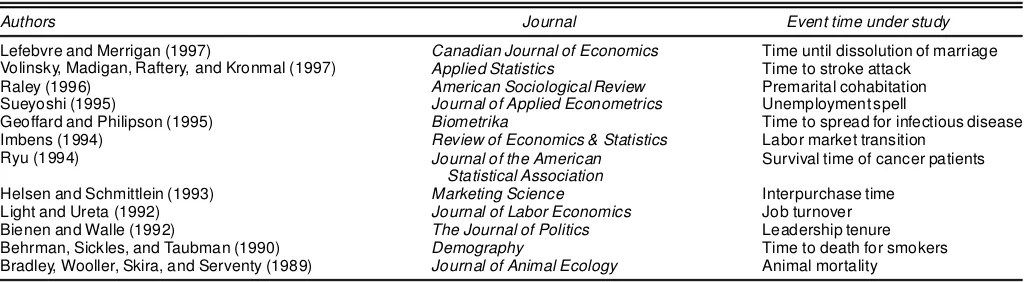
detergent, the household’s purchase timing is likely to be also inuenced by marketing variables in the product category (e.g., price, advertising). A statistical model that is well suited to cap-ture both of these feacap-tures of purchase-timingdata (i.e., intrinsic temporal purchase patterns and the effects of marketing vari-ables) is theproportional hazard model(PHM) rst proposed by Cox (1972) and used in an extensive range of applications to study event times. Table 1 gives a select review of recent appli-cations of the PHM in various disciplines.
Empirical studies in recent years have largely used the PHM to characterize purchase-timing behavior of households (Jain
and Vilcassim 1991, 1994; Vilcassim and Jain 1991; Gupta 1991; Helsen and Schmittlein 1993; Gonul and Srinivasan 1993; Wedel, Kamakura, Desarbo, and Hofstede 1995; Chin-tagunta and Haldar 1998; Hofstede and Wedel 1999; Chiang, Chung, and Cremers 2002). In these studies the construct of interest is a household’s instantaneous probability of making a purchase in a product category, conditional on the elapsed time since the household’s previous purchase in the product category. This conditional probability, also called the
haz-ard function, is multiplicatively decomposed into two
com-ponents: thebaseline hazard, which captures the household’s intrinsic temporal purchase pattern, and thecovariate function, which captures the inuence of marketing variables. In other words, the baseline hazard characterizes the distribution of the household’s interpurchase times after controlling for the effects of marketing variables.
Although the observed times of a household’s purchases in a product category are the events of central interest in the PHM formulation, the observed times of a household’s nonpurchases in the product category (i.e., shopping trips that result in non-purchase of the product category) contain useful information
© 2003 American Statistical Association Journal of Business & Economic Statistics July 2003, Vol. 21, No. 3 DOI 10.1198/073500103288619025
368
Table 1. A Select Review of Recent Applications of the PHM in Various Academic Disciplines
Authors Journal Event time under study
Lefebvre and Merrigan (1997) Canadian Journal of Economics Time until dissolution of marriage
Volinsky, Madigan, Raftery, and Kronmal (1997) Applied Statistics Time to stroke attack
Raley (1996) American Sociological Review Premarital cohabitation
Sueyoshi (1995) Journal of Applied Econometrics Unemployment spell
Geoffard and Philipson (1995) Biometrika Time to spread for infectious disease
Imbens (1994) Review of Economics & Statistics Labor market transition
Ryu (1994) Journal of the American Survival time of cancer patients
Statistical Association
Helsen and Schmittlein (1993) Marketing Science Interpurchase time
Light and Ureta (1992) Journal of Labor Economics Job turnover
Bienen and Walle (1992) The Journal of Politics Leadership tenure
Behrman, Sickles, and Taubman (1990) Demography Time to death for smokers
Bradley, Wooller, Skira, and Serventy (1989) Journal of Animal Ecology Animal mortality
as well. For example, knowing that a household made a shop-ping trip on a given week but did not purchase the product cate-gory is useful information from the standpoint of estimating the household’s responsiveness to marketing variables at the store (Chiang and Lee 1992). Furthermore, a household undertakes shopping trips in discrete intervals of time, often weekly, which makes the household’s purchase timing in a particular product category conditional on the household’s discrete time interval of shopping. In fact, it has been empirically documented that households’ shopping trips tend to be in increments of weeks (Dunn, Reader, and Wrigley 1983; Kahn and Schmittlein 1989; Chiang et al. 2002). The weekly nature of households’ shop-ping trips, coupled with the fact that not all shopshop-ping trips in-volve purchase of the product, makes the discrete-time version of the PHM (also called “grouped PHM”) more suitable to an-alyze purchase-timing data. Such a discrete-time version of the PHM, rst proposed by Thompson (1977), has been used with purchase-timing data by Gupta (1991) and Helsen and Schmit-tlein (1993). The continuous-time version of the PHM (as in Cox 1972) has been used by Jain and Vilcassim (1991) and Vil-cassim and Jain (1991). No previous studies have compared the discrete-time and continuous-time versions of the PHM using empirical data, although Wheat and Morrison (1990) have doc-umented that the “whether or not to buy” specication is su-perior to the “when to buy” specication in purchase timing models. This is the rst objective of this study.
Whereas the PHM species that the household’s hazard func-tion is multiplicatively decomposable as two components, the baseline hazard and the covariate function, the PHM remains silent on what parametric specication to use for the baseline hazard. In other words, there is no prescription as to which probability distribution is the most appropriate for character-izing interpurchase times. In the past, researchers have used various distributions for interpurchase times, including expo-nential, Weibull, and Erlang 2. Because one may not know a priori which probability distribution is the most appropriate for the available dataset, testing alternative parametric specica-tions for the baseline hazard becomes necessary. Alternatively, one may use a exible baseline hazard specication that permits various shapes. One such exible specication is thequadratic
Box–Cox specication, rst proposed by Flinn and Heckman
(1982) and later used by Jain and Vilcassim (1991). Another exible specication is theexpo-power specication, recently proposed by Saha and Hilton (1997) to study equipment failure
times, which allows the baseline hazard to be monotonically increasing, decreasing, U-shaped, or inverted-U-shaped. This is the exible baseline hazard specication used in this study. In fact, we compare the empirical performance of ve differ-ent parametric specications—expondiffer-ential, Weibull, Erlang 2, log-logistic, and expo-power—to understand which is the most appropriate for purchase-timing data. This is the second objec-tive of this study.
Whereas the discrete-time version of the PHM accounts for shopping trips that do not involve purchase of the product, it treats the household’s probability of purchasing the product at a given time to be independent of whether or not the household purchased the product on its previous shopping trip. Instead, the household’s probability of purchasing the product is assumed to depend only on the time elapsed since the household’s pre-vious purchase in the product category. This may not be a rea-sonable assumption. For example, a household’s likelihood of purchasing detergents during a shopping trip at timet, given previous purchase of detergents at timet¡2, may depend on whether or not the household undertook a shopping trip during timet¡1. Toward this end, one could use thecompeting-risks
hazardsframework of Hoel (1972) to distinguish between four
types of hazard functions for a household, that is, representing all possible transitions between purchase and no purchase on successive shopping trips of a household.This has not been pre-viously done in the PHM literature on purchase timing. We ad-dress this gap in the literature by employing thecause-specic
competing-risks hazard framework of Holt (1978) and Prentice et al. (1978) that distinguishes between two possible transitions on successive shopping trips, that is, no purchase to purchase, and purchase to purchase. This is the third objective of this study.
The estimates of the parameters of the covariate function— which, in our case, represent households’ sensitivities to mar-keting variables—are likely to be quite sensitive to the chosen parametric form of the baseline hazard (Trussell and Richards 1985). For example, the estimated price elasticity of detergents may be different depending on whether an exponential or a Weibull specication was used for the baseline hazard. One way to avoid potential misspecication of the baseline hazard is to impose no parametric form on it whatsoever, and instead estimate the baseline hazard nonparametrically. One such non-parametric approach, rst proposed by Prentice and Gloeck-ler (1978) and subsequently applied to economic data on
unemployment spells by Meyer (1990) and Han and Haus-man (1990), has been recently applied to purchase-timing data by Jain and Vilcassim (1994) and Wedel et al. (1995). In this approach, the baseline hazard is assumed to be a step
functionof time, (i.e., constant within a given day and
vary-ing from one day to another) and can be freely estimated using the available data. One disadvantage of such a non-parametric PHM approach is that the number of estimable parameters may increase signicantly, especially with purchase-timing data that involve long interpurchase times (say, 20–30 weeks). Another disadvantage of the nonparametric PHM ap-proach is its reliance on the researcher’s subjective choice of the time interval within which the baseline hazard will be as-sumed to be constant (such as day or week), especially when there are no theoretical prescriptions on the optimal choice of time interval. Whether or not these disadvantages outweigh the benets that accrue from avoiding parametric misspeci-cation of the baseline hazard is an empirical question. We answer this question by comparing the estimates of a nonpara-metric PHM with the estimates of the traditional paranonpara-metric PHM (with various parametric specications for the baseline hazard, as discussed earlier). This is the fourth objective of this study.
Last, but not least, the PHM must be allowed to be het-erogeneous across households to avoid potential bias in the parameter estimates of the baseline hazard and the covariate function. One way to exibly accommodate the effects of such unobserved heterogeneity in the PHM is to allow the intercept parameter of the covariate function to follow a discrete distrib-ution across households, whose locations and masses are freely estimated using the available data (Heckman and Singer 1984). Using scanner panel data, for which the number of households is quite large (a few hundred), and discrete choice models of brand choices, marketing researchers have found unobserved heterogeneity not only in the intercept parameter, but also in the slope parameters, that is, the covariate coefcients (Allenby and Rossi 1999). In line with this body of empirical work, we allow all of the parameters of the PHM (rather than the intercept parameter only) to be heterogeneous across households. This allows us to fully quantify the extent of unobserved heterogene-ity in households’ purchase-timing behavior, unlike previous studies that focused exclusively on single-parameter opera-tionalizations of unobserved heterogeneity. To the extent that each support of the heterogeneity distribution can be interpreted to represent a segment of households in the market, as is com-monly done in the economics and marketing literatures, the het-erogeneous PHM can be used by a rm to segment the market for its product and then develop differentiated marketing strate-gies, if possible. This is the fth objective of this study.
To summarize, our study has ve empirical objectives:
1. Compare continuous-time and discrete-time versions of the PHM
2. Compare various parametric specications—exponential, Weibull, Erlang-2, log-logistic, and expo-power—of the base-line hazard
3. Compare the single-risk formulation of the PHM with the (cause-specic) competing-risks formulation
4. Compare the parametric PHM with the nonparametric PHM
5. Compare the homogeneous PHM with the heterogeneous PHM.
To achieve these ve objectives, we estimate a whole range of specications of the PHM (that differ along the ve dimen-sions mentioned earlier) using scanner panel data from two dif-ferent product categories, laundry detergents and paper towels. In doing this, we not only glean some generalizable insights on households’ purchase-timing behavior, but also (more impor-tantly) lay out a general econometric framework that will be useful for empirical researchers who want to use the PHM for empirical work.
Since the last comprehensive treatise on the PHM—an ex-cellent tutorial article written by Kiefer (1988)—a number of useful developments have occurred in the PHM literature. This article encapsulates these developments, and is meant to serve as an updated empirical article on the PHM. We hope that this article will serve a useful reference to researchers hop-ing to use the PHM in subject areas besides markethop-ing and economics. To foster an appreciation of the basic theory and scope of not only the PHM, but also other types of duration-time models, the reader is directed to the informative books by Kalbeisch and Prentice (1980), Lawless (1982), Allison (1984), Cox and Oakes (1984), Lancaster (1990), and Meeker and Escobar (1998).
The rest of the article is organized as follows. In the next section we develop various PHM formulations and their corre-sponding likelihood equations (useful for estimation). In Sec-tion 3 we present our empirical ndings. We conclude in Section 4 with a summary and directions for future research.
2. MODEL FORMULATION AND ESTIMATION
Model development proceeds in six steps. First, we derive the continuous-time PHM for analyzing purchase-timing data; second, we develop a discrete-time version of the PHM that can handle shopping trips involving no purchase in the product cat-egory; third, we discuss different parametric specications of the baseline hazard; fourth, we extend the discrete-time PHM to embody cause-specic competing risks; fth, we derive the nonparametric PHM; and sixth, we incorporate unobserved het-erogeneity.
2.1 Cox’s (1972) Proportional Hazard Model Applied to Purchase Timing Data
Cox’s (1972) PHM species a household’s instantaneous probability (also called the household’s hazard function) of making a purchase in a product category, conditional on the elapsed time (t) since the household’s previous purchase in the product category as follows:
hi.t;Xt/Dhi.t/¤Ãi.Xt/: (1)
Herehi.t;Xt/stands for householdi’s hazard function at timet,
Xtis a row-vector of covariates (i.e., product-specic marketing
variables, such as price, display, and feature, and household-specic variables, such as product inventory) facing household
i at time t, hi.t/ stands for householdi’s baseline hazard at
timet, andÃi.Xt/stands for householdi’s covariate function at
timet. In this multiplicative model, the baseline hazard repre-sents the probability distribution characterizing the household’s interpurchase times, and the covariate function shifts this base-line hazard up or down depending on the values of the covari-ates. We use the following functional form to represent the co-variate function:
Ãi.Xt/DeXt¯i; (2)
where¯irepresents a column-vector of parameters
correspond-ing to the covariates contained inXt. An alternative functional
form that has been used in the literature is the cumulative dis-tribution function (cdf) of a standard normal disdis-tribution (see Koop and Ruhm 1993). Our choice of functional form is dic-tated by the fact that the hazard function must always be non-negative. This yields the standard PHM,
h.t;Xt/Dh.t/¤eXt¯; (3)
where the subscriptihas been dropped for notational ease. The hazard function can also be written as
h.t;Xt/D
f.t;Xt/
1¡F.t;Xt/
; (4)
wheref.t;Xt/stands for theprobability density function(pdf)
corresponding to the householdi’s hazard function at time t
and F.t;Xt/ stands for the correspondingcumulative
distrib-ution function(cdf). This equation can be understood as
fol-lows. Whereas f.t;Xt/ stands for the household’s
(uncondi-tional) probability of buying the product at timet, 1¡F.t;Xt/
stands for the probability that the household has not bought the product until timet. Combining (3) and (4) yields
f.t;Xt/
1¡F.t;Xt/
Dh.t/¤eXt¯; (5)
where 1¡F.t;Xt/is also called thesurvivor function, that is,
the probability that the household “survives” a purchase until timet, represented byS.t;Xt/. Therefore, an alternative way of
writing (5) is
f.t;Xt/Dh.t/¤eXt¯¤S.t;Xt/: (6)
To simplify (5) to a more “estimation-friendly” form, we can rewrite it as
dF.t;Xt/
1¡F.t;Xt/
Dh.t/¤eXt¯ ¤dt; (7)
which is a rst-order differential equation that can be solved as
Z F.t;Xt/
where the lower limit of integration (i.e., 0) corresponds to the time of the household’s previous purchase in the product cate-gory. Solving this yields
Substituting from (10) in (6) yields the following estimable ver-sion of the continuous-time PHM:
f.t;Xt/Dh.t/¤eXt¯¤e¡
Rt
0h.u/¤eXu¯du; (11)
wheref.t;Xt/represents the probability density associated with
the purchase event that occurs at timetand covariate vectorXt.
The most commonly used parametric specication for h.t/
in the PHM literature is the Weibull distribution. Alternative parametric specications include the exponential, Erlang, log-logistic, log-normal, Gompertz, Raleigh, and inverse Gaussian distributions. Estimation of the parameters of this PHM at the individual level can proceed as follows. Suppose that a house-hold providesn interpurchase time observations in the prod-uct category, say,.t1;t2;t3; : : : ;tn/. Each of these interpurchase
times is associated with a covariate vector, yielding a stacked set of covariate vectors given by.X1;X2;X3; : : : ;Xn/. The
fol-lowing likelihood function can be maximized to estimate the parameters of the PHM at the individual-level:
LD
n
Y
jD1
f.tj¡tj¡1;Xj/; (12)
wherenrepresents the total number of purchases made by the household in the product category,tj stands for the calendar
time associated with purchasej, andf.¢/is given by (11). This is the estimation procedure adopted by Jain and Vilcassim (1991) and Vilcassim and Jain (1991). It is clear from (12) that this pro-cedure computes the likelihood function based on a household’s purchase observations only. However, a household undertakes shopping trips at discrete points of time, often weekly, which makes the household’s purchase timing in a particular product category conditional on the household’s discrete time interval of shopping. To accommodate this, we next derive a discrete-time version of the PHM and set up a likelihood function based on all of the household’s shopping trips, not just shopping trips that result in purchase of the product.
2.2 Discrete-Time Version of the Proportional Hazard Model
Because a household’s shopping trips occur at discrete time points (usually every week), we can rewrite (10) in discrete time as whereuis discrete time, measured in the time interval of shop-ping trips (usually weeks). In this formulation, the integral of (10) is replaced in part by a summation that is consistent with the empirical fact that marketing variables associated with a product category (contained inXt/stay constant within a given
week but vary from week to week. The household’s probability of purchasing the product in discrete timet(since the previous purchase), also called thediscrete-time hazard, is then given by
Pr.t;Xt/D1¡ where Pr.t;Xt/ represents the probability that the purchase
event will occur at discrete time t and covariate vector Xt.
Pr.t;Xt/is also called the discrete-time hazard, as opposed to
h.t;Xt/, which is called the continuous-time hazard. The
fol-lowing likelihood function can be maximized to estimate the parameters of the discrete-time PHM at the individual level,
LD
T
Y
vD1
Pr.v;Xv/±v¤[1¡Pr.v;Xv/]1¡±v; (15)
where ±v is an indicator variable that takes the value 1 if the
product is purchased by the household at shopping tripvand 0 otherwise, and Pr.v;Xv/ is the household’s probability of
purchasing the product at shopping tripv, given by (14). The discrete-time PHM, also called the grouped PHM, has been adopted by Gupta (1991) and Helsen and Schmittlein (1993) in their work and is preferable to the continuous-time PHM be-cause it explicitly accounts for nonpurchases. Next, we discuss alternative parametric specications for the baseline hazard.
2.3 Baseline Hazard Specications
Here we discuss ve alternative parametric specications of the baseline hazard and their properties.
1. Exponential
h.t/D° ;
S.t/De¡°t; (16)
where° >0. Also called the “memoryless hazard,” this base-line hazard isat.
where° >0. This baseline hazard has a monotonicallyincreas-ing shape and has a rich history in the marketmonotonicallyincreas-ing literature (see, e.g., Gupta 1991).
3. Weibull
h.t/D° ®.°t/®¡1;
S.t/De¡.°t/®; (18)
where ° ; ® >0. This baseline hazard can be at, monotoni-cally increasing, or monotonimonotoni-cally decreasing. Given its exi-bility over the exponential hazard, which it nests as a special case (when®D1), it is the most popular baseline hazard spec-ication in the PHM literature.
4. Log-logistic
where ° ; ® >0. This baseline hazard can be monotonically decreasing or inverted U-shaped, with a turning point at tD
.®¡1/1=®=°. This baseline hazard has been found to be more suitable for purchase-timing data than the Weibull and Erlang-2 baseline hazards by Chintagunta and Haldar (1998).
5. Expo-power
h.t/D° ®t®¡1eµt®;
S.t/De°µ[1¡eµt ®
]; (20)
where¸; ® >0. Recently proposed by Saha and Hilton (1997), this baseline hazard can be at, monotonically increasing, monotonically decreasing, U-shaped, or inverted U-shaped, with a turning point attD[.1¡®/=®µ]1=®. Given its exibil-ity, this baseline hazard is expected to dominate the other four baseline hazards for any available dataset.
We compare the aforementioned parametric specications of the baseline hazard in both the continuous version [eqs. (11) and (12)] and the discrete version [eqs. (14) and (15)] of the PHM. Other possible baseline hazards include lognormal, in-verse Gaussian, Gompertz, and generalized gamma. Although these provide no additional exibility over the aforementioned baseline hazards, they involve cumbersome numerical integra-tion to compute the survivor funcintegra-tion. The lognormal speci-cation has the same shape characteristics as the log-logistic, whereas the generalized gamma specication does not admit a U-shaped baseline hazard. Next we extend the discrete-time PHM to allow for cause-specic competing risks.
2.4 Modeling Cause-Specic Competing Risks
Whereas the discrete-time version of the PHM, given in (14) and (15), explicitly accounts for shopping trips that do not in-volve purchase of the product [by including the no-purchase probability 1¡Pr.t;Xt/in (15)], it treats the household’s
proba-bility of purchasing the product at a given time [i.e., Pr.t;Xt/] to
be independent of whether or not the household purchased the product on its previous shopping trip. We relax this assumption by estimating two cause-specic hazards, one hazard for the case when the household made a purchase during its previous shopping trip and another for the case when the household did not. These cause-specic hazards are
Prn.t;Xt/D1¡e¡e where all of the variables are as explained in (14), except that the subscriptnstands for the case when the household’s shop-ping trip at time t¡1 involved no purchase of the product, whereas the subscriptp represents the case when the house-hold’s shopping trip at time t¡1 involved purchase of the product. Correspondingly, the likelihood function that can be maximized to estimate the parameters of the cause-specic haz-ards at the individual-levelis
where ±n is an indicator variable that takes the value 1 if the
product was not purchased by the household at shopping trip
v¡1 and 0 otherwise, and Prn.v;Xv/and Prp.v;Xv/are given
by (21). This formulation involves twice as many estimable pa-rameters as the formulation in (15). Cause-specic competing
risks have not been previously estimated with purchase-timing data and are proposed in this study for the rst time. Gaynor et al. (1993) gave a statistical application of cause-specic com-peting risks. Gonul and Srinivasan (1993) used a destination-specic competing-risks formulation to model brand-switching behavior of households. In applications involving more than two possible competing states (e.g., switching between brands), such as the investigation of households’ brand switching over time, this framework can easily be extended to estimate more than two cause-specic hazards. Next, we discuss a nonpara-metric version of the discrete-time PHM.
2.5 Nonparametric Proportional Hazard Model
The estimates of the parameters.¯/of the covariate func-tion are likely to be quite sensitive to the chosen parametric form of the baseline hazard. To avoid potential misspecication of the baseline hazard, we can impose no parametric form on it whatsoever, and estimate the baseline hazard nonparametri-cally (Prentice and Gloeckler 1978). This yields the discrete-time hazard
Pr.t;Xt/D1¡e¡e
Xt¯C®t
; (23)
where®tis a time-specic intercept-term that is allowed to vary
freely from one discrete time period (i.e., day) to another. (Note that the day is a superior time interval than the week, because households rarely undertake more than one shopping trip on the same day.) Comparing (23) with (14) shows that®t is the
logarithm of the integrated continuous baseline hazard,
®tDln
Z t t¡1
h.u/du: (24)
The likelihood function given in (15) can be maximized to es-timate the model parameters, except that we eses-timate all of the parameters in the step function.®1; ®2; : : : ; ®T/where T can
be very large. The value ofT is chosen based on the distribu-tion of observed interpurchase times in the data. For example, if purchases longer than 100 days are rarely observed, then we can reliably estimate no more than 100®t’s. This is in sharp
contrast to only a few (i.e., one, two, or three) parameters of the baseline hazardh.t/that need to be estimated in the parametric discrete-time PHM; see (14). Therefore, the additional exibil-ity offered by the nonparametric discrete-time PHM (compared with the parametric discrete-time PHM) comes at a cost—an increased number of estimable parameters. This nonparamet-ric approach has been used by Jain and Vilcassim (1994) and Wedel et al. (1995). Next, we discuss how to incorporate the effects of unobserved heterogeneity across households in the PHM.
2.6 Incorporating Unobserved Heterogeneity Across Households
We must allow the parameters of the PHM to be heteroge-neous across households to avoid potential bias in the parame-ter estimates of the baseline hazard and the covariate function (Lancaster 1979). One way to exibly accommodate the ef-fects of such unobserved heterogeneity in the PHM is to allow the parameters of the model to follow a multivariate discrete distribution across households, whose locations and masses
are estimated using the available data (Heckman and Singer 1984). Unlike previous studies on purchase timing that focused on single-parameter operationalizations of unobserved hetero-geneity (e.g., Jain and Vilcassim 1991), we allow all of the pa-rameters of the PHM to be heterogeneousacross households (as in Jensen 1993). We next give the likelihood equations for the heterogeneousversions of four types of PHM discussed earlier.
1. Continuous-time PHM
wherenh stands for the number of purchase occasions
corre-sponding to householdh,Sstands for the number of supports of the multivariate discrete distribution,psis the probability mass
associated with supports, and fs.¢/stands for the pdf of the
continuous-time PHM corresponding to supports,
fs.t;Xt/Dhs.t/¤eXt¯s¤e¡
Rt 0hs.u/¤eXu
¯s du
; (26)
wherehs.¢/stands for the baseline hazard correspondingto
sup-portsand¯sstands for the covariate parameters corresponding
to supports.
whereThstands for the number of shopping trips undertaken
by householdh, and Prs.¢/stands for the probability mass of
the discrete-time PHM associated with supports,
Prs.t;Xt/D1¡e¡e
cause-specic competing-risks PHM associated with supports,
Prns.t;Xt/D1¡e¡e
hazards associated with the two competing risks for supports, whereas¯ns and¯psstand for the covariate parameters
associ-ated with the two competing risks for supports. 4. Nonparametric PHM
where Prs.¢/stands for the probability mass of the
nonparamet-ric PHM associated with supports,
Prs.t;Xt/D1¡e¡e
Xt¯sC®ts
; (32)
where®ts stands for the log-integrated hazard at shopping trip
t, corresponding to supports.
This completes our exposition of various types of PHM spec-ications. Equations (25)–(32) present the estimable likelihood equations of these specications. These likelihood equations can be maximized using gradient-based techniques to obtain maximum likelihood estimates of model parameters.
Estimating the aforementioned heterogeneous specications involves a priori specication of the number of supportsS. Al-though the optimal value of S is not directly estimable, we start with the homogeneous specication (i.e.,SD1) and keep adding supports until model t stops improving, in terms of the Schwarz Bayesian criterion (SBC). Estimating the parameters for theSD1 case means that we can compare the results ob-tained using the heterogeneous version of a model with those obtained using its homogeneous counterpart.
One issue that deserves discussion is right censoring, that is, the spell of time between a household’s last purchase in the product category and the household’s last shopping trip. In the case of the continuous-time PHM, this can be handled by ex-plicitly including the survival probability for the right-censored spell in the household’s likelihood function,
LD
where th;last refers to the calendar time of the household’s last shopping trip. In the case of the discrete-time PHM, be-cause the household’s likelihood function is constructed using all of the household’s shopping trips, regardless of whether or not purchase occurred during a shopping trip, there is no right-censoring in the data.
3. EMPIRICAL RESULTS
We use scanner panel data from Information Resources In-corporated (IRI) on household purchases in a metropolitan mar-ket in a large U.S. city. For our analysis, we pick two product categories: laundry detergents and paper towels. We believe that the “weak separability” assumption (i.e., the assumption that households’ purchase decisions in a product category can be analyzed independently compared to their purchase decisions in other product categories in the store) is more reasonable for these product categories than for other product categories, such as soup or soft drinks. This is because there are no obvious substitutes or complements for either detergents or paper tow-els, and both products can be considered necessities for most households. These datasets cover a period of two years from June 1991 to June 1993 and contain shopping trip information on 494 panelists across four different stores in an urban market. For each product category, the dataset contains information on marketing variables—price, in-store displays, and newspaper
feature advertisements at the level of stock-keeping unit (SKU) for each store/week.
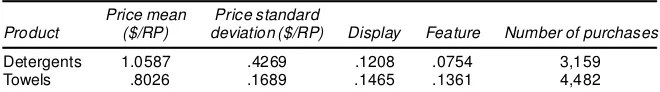
Choosing households that bought at the two largest stores in the market (that collectively account for 90% of all shopping trips in the database) yields 488 households. From these house-holds, we pick a random sample of 300 househouse-holds, yielding a total of 39,276 shopping trips at the two largest stores. This is done to keep the size of the dataset manageable. For those shopping trips in which a household visits the store but does not purchase a particular product category, we compute marketing variables as share-weighted average values across all SKUs in the product category, where shares are household-specic and computed using the observed purchases of the household over the study period. Computing marketing variables using such share-weighting has precedence in the marketing literature on category purchase models (see, e.g., Chib, Seetharaman, and Strijnev 2002). Descriptive statistics pertaining to the marketing variables in the two product categories are provided in Table 2. Price is in dollars per regular package size, and display and fea-ture are numbers between 0 and 1, representing the fraction of SKUs that were on display and feature.
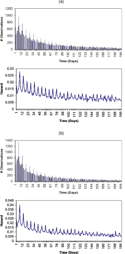
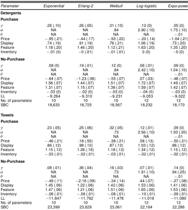
Both detergentsand towels appear to be displayed quite heav-ily at the store (about 35% of the time), whereas towels are featured in the Sunday newspaper more often (35%) than de-tergents (28%). The empirical distributions of observed inter-purchase times—specically, the frequency histogram and the empirical hazard—in the two product categories are plotted in Figure 1. The frequency distributions appear to have a mode close to 1 week (i.e., 7 days) and are skewed to the right. The empirical hazard functions appear to be monotonically decreas-ing. Interestingly, the empirical hazard shows peaks in multi-ples of 7 days. This is consistent with the empirical observation that households undertake shopping trips in weekly intervals (Dunn et al. 1983; Kahn and Schmittlein 1989; Chiang et al. 2002). The purpose of estimating the proposed PHM is to
es-timatethese density and hazard functionsafter accounting for
the effects of marketing variables.
We estimate the following PHM formulations:
² Model 1, continuous-time PHM ² Model 2, discrete-time PHM
² Model 3, cause-specic, competing-risks, discrete-time PHM
² Model 4, nonparametric PHM.
For models 1, 2, and 3, we test ve different specications of the baseline hazard: exponential, Erlang-2, Weibull, log-logistic, and expo-power. For model 4, we parameterize the nonparamet-ric baseline hazard [see (23) and (24)] using 100 time-specic intercepts.®1; ®2; : : : ; ®T/, because 90% of the masses of the
observed interpurchase time distributions are within 100 days (see Fig. 1).
Table 2. Descriptive Statistics on Marketing Variables (number of householdsD300; number of shopping tripsD39,276)
Price mean Price standard
Product ($/RP) deviation ($/RP) Display Feature Number of purchases
Detergents 1.0587 .4269 .1208 .0754 3,159
Towels .8026 .1689 .1465 .1361 4,482
(a)
(b)
Figure 1. Observed Interpurchase Times for (a) Detergents and (b) Towels.
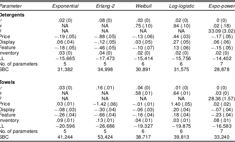
Table 3 gives the parameter estimates for model 1, that is, continuous-time PHM. Each column represents a different parametric specication of the baseline hazard (e.g., exponen-tial, Erlang-2, and so on). For each specication, along with the parameter estimates we report the maximized log-likelihood value (LL), the total number of parameters (n), and the SBC, which is dened as¡2¤LLC.lnT/¤n, whereTis the number of observations in the dataset. The SBC allows us to compare model ts across different specications after adjusting for the number of parameters in each specication.
If we rank-order the ve baseline hazard specications in terms of SBC, the expo-power specication nishes the best among the ve. In terms of the parameters associated with the marketing variables, we would expect the price parameter to have a negative sign; that is, the higher the price of the prod-uct, the lower the household’s expected likelihood of purchas-ing the product. Likewise, we would expect the display and fea-ture parameters to have positive signs. But this does not appear to always be the case in Table 3. For example, in the detergents category, the price parameter is wrongly signed under the log-logistic specication, the display parameter is wrongly signed under the Erlang-2 specication, and the feature parameter is wrongly signed for all specications except the log-logistic. In the towels category, 11 of the 15 parameters associated with marketing variables are wrongly signed.This indicates that by not accounting for the effects of shopping trips that result in households’ nonpurchase of the product, the continuous-time
PHM wrongly estimates the effects of marketing variables.This
is conrmed by estimating the discrete-time PHM (model 2), which explicitly accounts for the effects of shopping trips in-volving nonpurchase of the product, as is explained later. In-ventory effects are expected to be negative; that is, the higher the household’s product inventory, the lower the household’s expected likelihood of purchasing the product. However, the parameter associated with the inventory variable is positively signed under all specications. Overall, these ndings suggest that the continuous-time PHM is a poor candidate to explain households’ purchase timing decisions in detergents and tow-els.
Table 4 gives the parameter estimates for model 2, (i.e., discrete-time PHM). Results are reported for ve different parametric specication of the baseline hazard. Unlike the continuous-time PHM, which treats purchases as events occur-ring in continuoustime, the discrete-time PHM treats purchases as events occurring in discrete time, specically during shop-ping trips.
If we rank-order the ve baseline hazard specications in terms of SBC, then the expo-power specication nishes the best for detergents, whereas the log-logistic nishes the best for towels. After we account for unobserved heterogeneity, as discussed later, it turns out that the expo-power specication nishes the best for towels as well. For both product categories, the parameters associated with display and feature are correctly (positively) signed under all specications, whereas the para-meter associated with price is correctly (negatively) signed un-der four of ve specications (i.e., all specications except log-logistic). These ndings are quite remarkable, consider-ing the incorrect signs associated with these parameters in the continuous-time PHM (i.e., model 1).This indicates that by ex-plicitly accounting for the effects of shopping trips that result in households’ nonpurchaseof the product, the discrete-time PHM is able to obtain superior estimates (in terms of face validity) of the effects of marketing variables compared to the
continuous-time PHM. The inventory parameter is also correctly
(nega-tively) signed under all specications. Overall, these ndings suggest that the discrete-time PHM is an excellent candidate to explain households’ purchase-timing decisions in detergents and towels. This is remarkably consistent with the prescription of Wheat and Morrison (1990) that the “whether or not to buy”
Table 3. Parameter Estimates and Standard Errors for Model 1 (continuous-time PHM)
Parameter Exponential Erlang-2 Weibull Log-logistic Expo-power
Detergents
° .02 (0) .08 (0) .03 (0) .02 (0) 0 (0)
® NA NA .75 (.10) .94 (.10) .02 (.18)
µ NA NA NA NA 33.09 (3.02)
Price ¡:19 (.05) ¡:88 (.05) ¡:13 (.06) .44 (.03) ¡:17 (.05)
Display .06 (.04) ¡:12 (.05) .03 (.05) .27 (.05) .06 (.06)
Feature ¡:18 (.05) ¡:46 (.05) ¡:10 (.07) .13 (.06) ¡:15 (.05)
Inventory .03 (0) .04 (0) .02 (0) .02 (0) .02 (0)
LL ¡15;665 ¡17;473 ¡15;414 ¡15;756 ¡14;402
No. of parameters 5 5 6 6 7
SBC 31,382 34,998 30,891 31,575 28,878
Towels
° .03 (0) .16 (.01) .04 (0) .01 (0) 0 (0)
® NA NA .58 (.01) .64 (.01) .03 (0)
µ NA NA NA NA 28.36 (1.57)
Price .03 (.01) ¡1:42 (.06) ¡:01 (.01) 1.40 (.05) .02 (.02)
Display ¡:08 (.03) ¡:30 (.04) ¡:06 (.03) .20 (.04) ¡:07 (.04)
Feature ¡:26 (.04) ¡:66 (.04) ¡:16 (.04) .18 (.04) ¡:23 (.04)
Inventory .09 (.01) .13 (.01) .04 (.01) .03 (.01) .08 (.01)
LL ¡20;596 ¡26;686 ¡19;327 ¡19;875 ¡16;583
No. of parameters 5 5 6 6 7
SBC 41,244 53,424 38,717 39,813 33,240
specication must be preferred to the “when to buy” specica-tion in purchase-timing models.
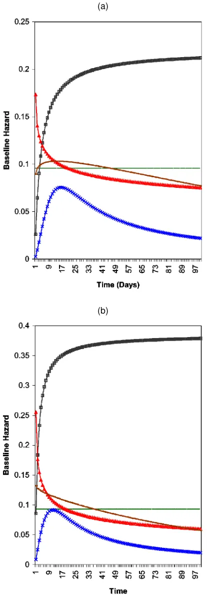
The estimated discrete-time baseline hazards [i.e., 1¡S.t/=
S.t¡1/] for the discrete-time PHM are plotted in Figure 2. Except for Erlang-2 (that can allow only for a monotonically increasing baseline hazard), all of the other parametric spec-ications indicate, by and large, a monotonically decreasing shape for the baseline hazard. Even the log-logistic specica-tion, which can allow only for an inverted U-shape, reaches its maximum quickly (at 17 days for detergents and at 10 days for towels) and starts decreasing thereafter. The expo-power spec-ication exhibits a monotonically decreasing shape for towels and an inverted U-shape, with a peak at about 10 days, for tow-els. The shape becomes nonmonotonic once heterogeneity is
accounted for, as is shown later. Given the exibility of the expo-power specication over the others (i.e., it can take on a rich variety of shapes), it appears to be a good candidate for baseline hazard specication in the PHM in general.
Table 5 gives the parameter estimates for model 3 (cause-specic competing-risks PHM). Results are reported for ve different parametric specications of the baseline hazard. Model 3 is different from model 2 in that it distinguishes be-tween purchase events preceded by nonpurchase and purchase events preceded by purchase. In other words, model 2 assumes the household’s discrete-time hazard for purchase timing to be the same at a shopping trip, regardless of whether or not a purchase occurred in the household’s previous shopping trip.
Table 4. Parameter Estimates and Standard Errors for Model 2 (discrete-time PHM)
Parameter Exponential Erlang-2 Weibull Log-logistic Expo-power
Detergents
° .10 (0) .25 (0) .14 (0) .07 (0) .09 (0)
® NA NA .84 (.05) 2.23 (.10) 1.06 (.20)
µ NA NA NA NA ¡:01 (0)
Price ¡:71 (.07) ¡1:40 (.06) ¡:61 (.07) .11 (.09) ¡:55 (.06)
Display 1.48 (.07) 1.33 (.07) 1.42 (.07) 1.65 (.07) 1.41 (.07)
Feature 1.29 (.07) 1.14 (.07) 1.35 (.07) 1.65 (.07) 1.40 (.07)
Inventory ¡:02 (0) ¡:02 (0) ¡:02 (0) ¡:03 (0) ¡:02 (0)
LL ¡9;344 ¡9;487 ¡9;268 ¡9;188 ¡9;153
No. of parameters 5 5 6 6 7
SBC 18,740 19,026 18,599 18,439 18,380
Towels
° .10 (.01) .49 (.02) .19 (.01) .10 (0) .14 (0)
® NA NA .73 (.05) 2.03 (.10) .98 (.25)
µ NA NA NA NA ¡:01 (0)
Price ¡:53 (.11) ¡2:29 (.07) ¡:36 (.12) .36 (.06) ¡:31 (.13)
Display 1.36 (.06) 1.12 (.05) 1.31 (.06) 1.42 (.06) 1.30 (.06)
Feature 1.41 (.06) 1.14 (.05) 1.45 (.06) 1.59 (.06) 1.46 (.06)
Inventory ¡:05 (.01) ¡:03 (.01) ¡:07 (.01) ¡:07 (.01) ¡:07 (.01)
LL ¡11;906 ¡12;220 ¡11;533 ¡11;173 ¡11;298
No. of parameters 5 5 6 6 7
SBC 23,864 24,492 23,129 22,409 22,670
(a)
(b)
Figure 2. Estimated Baseline Hazards—Discrete-Time PHM (Model 2) for (a) Detergents and (b) Towels (- - - expo; —¥— Erlang-2; —N— Wellbull; —-£—- log-logistic; ——- expo-power).
Model 3 relaxes this assumption and estimates two separate hazard functions.
Table 5 reports the parameters associated with the
purchase-to-purchaseand the no purchase-to-purchasetransitions. By
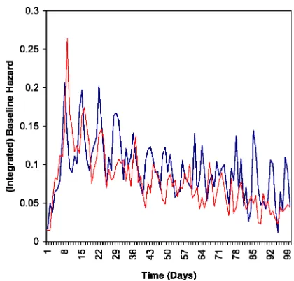
and large, the parameter estimates associated with the purchase-to-purchase transition have larger standard errors than those as-sociated the no purchase-to-purchase transition in both prod-uct categories. This is in line with the empirical fact that a much larger number of observations are associated with the no purchase-to-purchase transition in the data. In the deter-gents category, there are 2,683 no purchase-to-purchase tran-sitions and 453 purchase-to-purchase trantran-sitions. In the towels category, there are 3,449 no purchase-to-purchase transitions and 988 purchase-to-purchase transitions. The parameter asso-ciated with display is higher in magnitude for the no purchase-to-purchase transition under all specications. This indicates that store displays, to the degree that they serve as a “cue” to shoppers to remind them to buy a product, are less impor-tant when shoppers have just bought the product during their previous shopping trip. The parameter associated with product inventory is also higher in magnitude for the no purchase-to-purchase transition, especially for towels. This can be rational-ized using the argument that to the degree that product inventory levels are likely to be higher during shopping trips immediately after purchase of the product, they are less likely to drive pur-chase during such shopping trips. Next, we plot the estimated baseline hazards for the two cause-specic transitions under the expo-power specication. These plots are given in Figure 3.
The baseline hazard for the purchase-to-purchase transi-tion is inverted U-shaped, whereas that for the no purchase-to-purchase transition is monotonically decreasing. In other words, given that a household buys the product on a shop-ping trip, the household’s probability of buying the product in the future, conditional on not buying until then, increases for about 10 days and then begins to decrease. In contrast, given that a household does not buy the product on a shopping trip, the household’s probability of buying the product in the future, conditional on not buying until then, steadily decreases. These ndings highlight the importance of distinguishing between two types of causes (i.e., purchase versus nonpurchase during the previous shopping trip) while estimating the discrete-time PHM. This is a new nding in the literature on purchase-timing models.
In Table 4, the estimates of the parameters of the marketing variables appear to be quite sensitive to the chosen parametric form of the baseline hazard. One way to avoid potential mis-specication of the baseline hazard is to impose no parametric form on it whatsoever, and instead estimate the baseline hazard nonparametrically. Consistent with this approach, we assume the integrated baseline hazard to be astep functionof time and estimate the parameters of this step function using the available data [see (23) and (24)]. The results of the nonparametric PHM are given in Table 6.
The estimates of the parameters associated with marketing variables are remarkably similar to those obtained using the parametric, discrete-time PHM (see Table 3). However, given the much larger number of estimable parameters in the non-parametric PHM, its SBC criterion (that penalizes a highly pa-rameterized model) is worse then the parametric, discrete-time PHM. For towels, for example, all parametric specications ex-cept Erlang-2 (see Table 3) t better than the nonparametric PHM. The estimated nonparametric baseline hazards, plotted in Figure 4, are nonmonotonic and peak at about 10 days, which
Table 5. Parameter Estimates and Standard Errors for Model 3 (cause-specic, competing-risks, discrete-time PHM)
Parameter Exponential Erlang-2 Weibull Log-logistic Expo-power
Detergents
Purchase
° .26 (.10) .26 (.05) .31 (.10) .12 (0) .05 (0)
® NA NA .84 2.90 (.10) 1.75 (.10)
µ NA NA NA NA ¡:01
Price ¡:95 (.21) ¡:44 (.17) ¡:93 (.22) ¡:20 (.14) ¡1:04 (.21)
Display .74 (.19) .91 (.19) .76 (.21) 1.06 (.19) .73 (.20)
Feature 1.18 (.20) 1.46 (.20) 1.12 (.21) 1.63 (.20) 1.35 (.20)
Inventory ¡:01 (0) ¡0 (.01) ¡:01 (.01) 0 (0) ¡0 (0)
No-Purchase
° .08 (0) .19 (.01) .12 (0) .06 (.01) .09 (0)
® NA NA .84 2.42 (.10) 1.04 (.10)
µ NA NA NA NA ¡:01
Price ¡:64 (.07) ¡1:23 (.06) ¡:55 (.07) .07 (.03) ¡:48 (.07)
Display 1.56 (.07) 1.44 (.07) 1.51 (.07) 1.72 (.07) 1.49 (.07)
Feature 1.31 (.07) 1.15 (.07) 1.38 (.07) 1.59 (.07) 1.42 (.07)
Inventory ¡:03 (0) ¡:02 (0) ¡:03 (0) ¡:04 (0) ¡:03 (0)
LL ¡9;264 ¡9;310 ¡9;231 ¡9;053 ¡9;022
No. of parameters 10 10 10 12 12
SBC 18,633 18,725 18,567 18,232 18,170
Towels
Purchase
° .23 (.05) .25 (.06) .32 (.05) .12 (.01) .09 (0)
® NA NA .73 2.56 (.10) 1.50 (.20)
µ NA NA NA NA ¡:01
Price ¡:46 (.21) .18 (.55) ¡:38 (.21) .58 (.13) ¡:50 (.21)
Display .86 (.12) .98 (.12) .87 (.12) 1.03 (.12) .86 (.12)
Feature 1.15 (.12) 1.26 (.16) 1.18 (.12) 1.34 (.12) 1.15 (.12)
Inventory ¡:03 (.01) ¡:02 (.01) ¡:03 (.01) ¡:02 (.01) ¡:02 (.01)
No-Purchase
° .08 (.01) .36 (.04) .16 (.03) .07 (.01) .14 (0)
® NA NA .73 1.91 (.10) .94 (.25)
µ NA NA NA NA ¡:01
Price ¡:49 (.11) ¡2:16 (.09) ¡:34 (.14) .44 (.07) ¡:27 (.08)
Display 1.45 (.06) 1.22 (.06) 1.42 (.06) 1.53 (.06) 1.41 (.06)
Feature 1.47 (.06) 1.21 (.06) 1.51 (.06) 1.65 (.06) 1.53 (.06)
Inventory ¡:08 (.01) ¡:06 (.01) ¡:08 (.01) ¡:10 (.01) ¡:09 (.01)
LL ¡11;647 ¡11;762 ¡11;478 ¡11;019 ¡11;080
No. of parameters 10 10 10 12 12
SBC 23,399 23,629 23,061 22,164 22,286
is consistent with the log-logistic and expo-power baseline haz-ards shown in Figure 2. Given the similarity in ndings be-tween exible parametric specications and the nonparametric specication of the PHM, there does not appear to be a justi-able benet to using the nonparametric PHM on the availjusti-able purchase-timing data.
Last, but not least, we investigate the consequences of ac-commodating unobserved heterogeneity in model parameters across households. Table 7 gives the parameter estimates of the heterogeneous versions of model 2, where we use a three-support heterogeneity distribution and estimate the locations and masses of each support using the purchase-timing data. Model ts (in terms of the SBC) dramatically improve after ac-counting for unobserved heterogeneity across households. The parameters associated with marketing variables show consid-erable variation across the three supports of the heterogeneity distribution. For example, under the expo-power specication, the price parameters associated with the three supports of prob-ability masses .43, .39, and .18 are¡3:39,¡2:70, and¡1:12.
Contrasting with the estimated price coefcient of¡:31 under the homogeneous expo-power specication (the last column of Table 4), one can conclude that failing to account for the ef-fects of unobserved heterogeneity substantially understates the effectiveness of price in the product category.
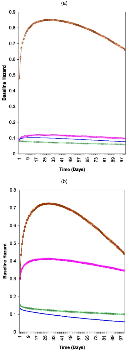
To better understand the extent of unobserved heterogene-ity in the estimated baseline hazards, we plot the expo-power baseline hazards for the three supports of the heterogeneity dis-tribution (along with the baseline hazard estimated in the homo-geneous specication) in Figure 5. For both product categories, we nd signicant heterogeneity in the estimated baseline haz-ards. In the detergents category, the baseline hazard associated with the third support (with mass 10%) has an inverted U-shape, peaking at about 25 days, whereas the baseline hazards as-sociated with the rst two supports are both monotonically decreasing and lower than the former. The baseline hazard as-sociated with the homogeneous specication is monotonically decreasing and lies between the baseline hazards of the rst and second supports. In the towels category, the baseline hazards
(a)
(b)
Figure 3. Estimated Cause-Specic Baseline Hazards (Model 3) for (a) Detergents and (b) Towels (—— Purchase; —-£—- Nonpurchase).
associated with the second and third supports (that have a col-lective mass of 61%) are both inverted U-shaped and both peak at about 25 days, with the second support’s baseline hazard lower in height. The baseline hazard associated with
Figure 4. Estimated Nonparametric Baseline Hazards (Model 4) (——– detergents; - - - towels).
the rst support (with mass 39%) is monotonically decreasing over time. The baseline hazard associated with the homoge-neous specication is monotonically decreasing and lower than the baseline hazards of the three supports of the heterogeneous specications. This means that the homogeneous specication incorrectly estimates not only the shape but also the mag-nitude of the baseline hazard. These ndings underscore the importance of incorporating unobserved heterogeneity in all parameters of the PHM. Our ndings about nonmonotonic discrete-time baseline hazards are consistent with the ndings of Helsen and Schmittlein (1993).
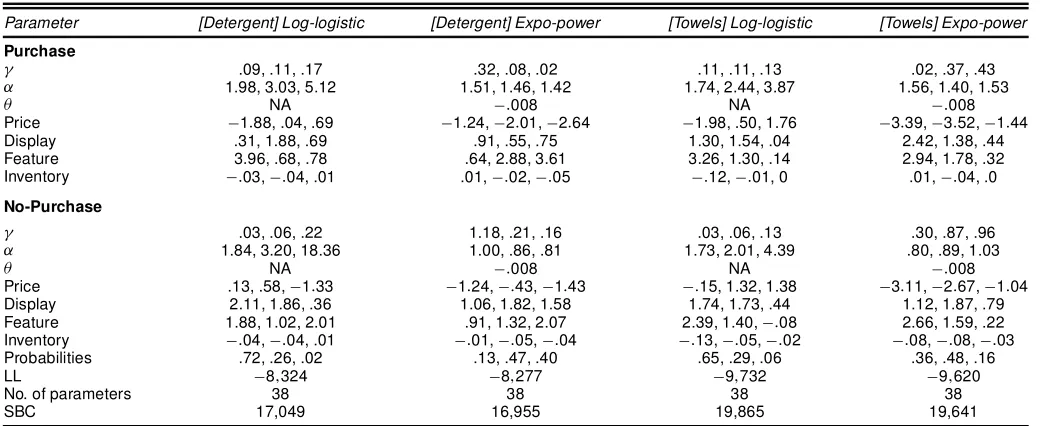
Table 8 gives the parameter estimates of the heterogeneous versions of model 3. It is clear from the improvement in model t going from its homogenous counterpart that accommodating
Table 6. Parameter Estimates and Standard Errors for Model 4 (nonparametric PHM)
Parameter Detergent (Homogeneous) Towels (Homogeneous) Detergent (Heterogeneous) Towels (Heterogeneous)
Baseline hazard See Figure 4 See Figure 4 See Figure 6 See Figure 6
Price ¡:58 (.07) ¡:30 (.06) ¡1:71,¡:76,¡2:30 ¡1:14,¡2:93,¡3:66
Display 1.41 (.07) 1.30 (.07) .85, 1.82, 1.65 .75, 1.72, 1.28
Feature 1.45 (.07) 1.48 (.07) .75, 1.26, 1.81 .24, 1.68, 2.37
Inventory ¡:03 (0) ¡:07 (0) 0,¡:03,¡:03 ¡:01,¡:04,¡:09
LL ¡8;947 ¡11;021 ¡8;007 ¡9;395
No. of parameters 104 104 116 116
SBC 18,994 23,142 17,241 20,017
Table 7. Results for Heterogeneous Model 2 (discrete-time PHM)
Parameter [Detergent] Log-logistic [Detergent] Expo-power [Towels] Log-logistic [Towels] Expo-power
° .02, .04, .13 .08, .09, .64 .04, .02, .14 .17, .36, .36
® 1.52, 1.98, 4.19 .99, 1.09, 1.31 1.74, 1.39, 3.49 .96, 1.12, 1.36
µ NA ¡:003 NA ¡:003
Price ¡:39, .66, .30 ¡1:72,¡:61,¡1:63 .70,¡:51, .85 ¡3:39,¡2:70,¡1:12
Display 2.15, 2.11, 1.38 1.58, 1.79, .85 2.08, 1.05, 1.08 1.26, 1.68, .73
Feature 2.54, 1.48, 1.20 1.94, 1.25, .80 2.20, 3.24, .47 2.35, 1.59, .24
Inventory ¡:02,¡:05,¡:01 ¡:03,¡:04, .00 ¡:05,¡:31,¡:02 ¡:11,¡:05,¡:01
Probabilities .38, .51, .11 .46, .44, .10 .43, .39, .18 .39, .46, .15
LL ¡8;379 ¡8;184 ¡9;791 ¡9;574
No. of parameters 20 20 20 20
SBC 16,969 16,579 19,793 19,359
(a)
(b)
Figure 5. Estimated Baseline Hazards—Discrete-Time PHM (Model 2) for (a) Detergents and (b) Towels (—¨— support 1; —N— support 2; —¥— support 3; ——- homogeneous).
unobserved heterogeneity in model parameters is very impor-tant in model 3 as well. Columns 4 and 5 of Table 6 give the parameter estimates of the heterogeneous versions of model 4. Comparing the empirical performance of the heterogeneous
versions of models 2, 3, and 4 further corroborates the ndings obtained earlier using their homogeneous counterparts.
3.1 Predictive Validation
To assess the predictive performance of the various base-line hazard specications, we perform a validation task using a holdout sample. Specically, we reestimate the heterogeneous versions of models 1, 2, and 3 using purchase data from 250 households, then compute the validation log-likelihoods for the observed interpurchase times for the remaining 50 households in the data. Table 9 gives the results of this validation exer-cise. The holdout validation results are quite consistent with in-sample estimation results, that is, model 2 (discrete-time PHM) validates holdout purchases much better than model 1 (continuotime PHM). However, validation gains from us-ing model 3 (cause-specic, competus-ing risks, discrete-time PHM) instead of model 2 appear to be only marginal. Within each model, the expo-power and log-logistic specications for the baseline hazard validate holdout purchases better than the other three specications. The nonparametric PHM validates the holdout data better than the other models. Overall, the hold-out validation results corroborate our estimation-basedndings, especially those pertaining to the relative performance of the various PHM specications.
4. CONCLUSIONS
We have discussed using the PHM to study households’ in-terpurchase times with laundry detergents and paper towels. We compared the empirical performance of continuous-time and discrete-time PHMs and found the latter to be superior in terms of both model t and face validity of the estimated parame-ters, because it explicitly accounts for shopping trips that do not involve purchase of the product. We compare ve speci-cations of the baseline hazard and nd the recently proposed expo-power specication to t and validate the data better than the other specications. We then estimate cause-specic com-peting risks, where we distinguish between two types of pur-chase events based on whether or not the shopping trip imme-diately preceding the purchase also involved a purchase. Such a competing-risks specication ts the observed data better than a discrete-time PHM that does not make such a distinc-tion. We estimate a nonparametric version of the PHM that in-volves many more parameters than the parametric version, and nd that the additional exibility afforded by the nonparametric baseline hazard does not alter the conclusions obtained using a exible, parsimonious parametric specication. Finally, we in-corporate unobserved heterogeneity by allowing all of the para-meters of the PHM to follow a multivariate discrete distribution across households, and nd evidence of substantial heterogene-ity in the marketplace.
Other examples of applications involving multiple event times at the individual level with time-varying covariates are in-dividuals changing jobs over time, inin-dividualsgetting promoted within their organization over time, and companies changing advertising agencies over time. For researchers working on such datasets, this article will be a useful resource for possible model specications. At this point, some caveats are in order. First, we
Table 8. Results for Heterogeneous Model 3 (cause-specic, competing-risks, discrete-time PHM)
Parameter [Detergent] Log-logistic [Detergent] Expo-power [Towels] Log-logistic [Towels] Expo-power
Purchase
° .09, .11, .17 .32, .08, .02 .11, .11, .13 .02, .37, .43
® 1.98, 3.03, 5.12 1.51, 1.46, 1.42 1.74, 2.44, 3.87 1.56, 1.40, 1.53
µ NA ¡:008 NA ¡:008
Price ¡1:88, .04, .69 ¡1:24,¡2:01,¡2:64 ¡1:98, .50, 1.76 ¡3:39,¡3:52,¡1:44
Display .31, 1.88, .69 .91, .55, .75 1.30, 1.54, .04 2.42, 1.38, .44
Feature 3.96, .68, .78 .64, 2.88, 3.61 3.26, 1.30, .14 2.94, 1.78, .32
Inventory ¡:03,¡:04, .01 .01,¡:02,¡:05 ¡:12,¡:01, 0 .01,¡:04, .0
No-Purchase
° .03, .06, .22 1.18, .21, .16 .03, .06, .13 .30, .87, .96
® 1.84, 3.20, 18.36 1.00, .86, .81 1.73, 2.01, 4.39 .80, .89, 1.03
µ NA ¡:008 NA ¡:008
Price .13, .58,¡1:33 ¡1:24,¡:43,¡1:43 ¡:15, 1.32, 1.38 ¡3:11,¡2:67,¡1:04
Display 2.11, 1.86, .36 1.06, 1.82, 1.58 1.74, 1.73, .44 1.12, 1.87, .79
Feature 1.88, 1.02, 2.01 .91, 1.32, 2.07 2.39, 1.40,¡:08 2.66, 1.59, .22
Inventory ¡:04,¡:04, .01 ¡:01,¡:05,¡:04 ¡:13,¡:05,¡:02 ¡:08,¡:08,¡:03
Probabilities .72, .26, .02 .13, .47, .40 .65, .29, .06 .36, .48, .16
LL ¡8;324 ¡8;277 ¡9;732 ¡9;620
No. of parameters 38 38 38 38
SBC 17,049 16,955 19,865 19,641
Table 9. Holdout Validation Results
Parameter Exponential Erlang-2 Weibull Log-logistic Expo-power Nonparametric
Detergents
Model 1 ¡3;109 ¡3;881 ¡2;962 ¡3;107 ¡2;475 NA
Model 2 ¡1;778 ¡1;797 ¡1;773 ¡1;761 ¡1;747 NA
Model 3 ¡1;792 ¡1;784 ¡1;789 ¡1;764 ¡1;753 NA
Model 4 NA NA NA NA NA ¡1;722
Towels
Model 1 ¡4;635 ¡7;620 ¡4;100 ¡4;221 ¡3;187 NA
Model 2 ¡2;691 ¡2;840 ¡2;570 ¡2;400 ¡2;486 NA
Model 3 ¡2;582 ¡2;633 ¡2;570 ¡2;337 ¡2;426 NA
Model 4 NA NA NA NA NA ¡2381
have adopted the likelihood-based perspective to estimating the parameters of the PHM. Recently, an important literature on Bayesian analysis of the PHM has developed. A discussion of this literature is beyond the scope of this article, and the reader is directed to the studies of Sinha (1993), Laud, Damien, and Smith (1998), and Kim and Lee (2001). Sinha (1993), for ex-ample, used the Markov chain Monte Carlo (MCMC) technique of Gibbs sampling to sample from the joint posterior distribu-tion of the parameters of the PHM. In our case, because the estimated nonparametric baseline hazard (see Fig. 4) appears to be quite volatile, a shrinkage estimator that shrinks the non-parametric hazard across periods may be a worthy avenue of in-vestigation. Second, it would be of interest to allow for a richer structure of unobserved heterogeneity,such as a mixture of nor-mals, to fully quantify the extent of unobserved heterogeneity in the marketplace, and use hierarchical Bayes procedures to estimate the parameters of the PHM at the household level (Al-lenby, Arora, and Ginter 1999). This would facilitate the devel-opment of marketing initiatives at the household level. Third, it may be useful to disentangle the effects of time-varying covariates (such as price) from the effects of time-invariant covariates (such as household demographics) on purchase tim-ing. Fourth, one could use discrete-time probability distribu-tions, such as geometric, Waring, and negative hypergeometric (Sengupta, Chatterjee, and Chakraborty 1995), instead of using
grouped versions of continuous-time density functions (as dis-cussed in this article) to model interpurchase times. Fifth, one can investigate possible nonstationarity of the parameters of the PHM over time (Imbens 1994). Sixth, it would be of interest to benchmark the PHM against the additive risk model of Aalen (1980).
ACKNOWLEDGMENTS
The authors thank Andrei Strijnev for setting up the datasets used in this article.
[Received February 2001. Revised June 2002.]
REFERENCES
Aalen, O. O. (1980), “A Model for Nonparametric Regression Analysis of Counting Processes,” inMathematical Statistics and Probability Theory, Lecture Notes in Statistics, Vol. 2, New York: Springer-Verlag, pp. 1–25. Allenby, G. M., Arora, N., and Ginter, J. L. (1998), “On the Heterogeneity of
Demand,”Journal of Marketing Research, 35, 384–389.
Allenby, G. M., Leone, R. P., and Jen, L. (1999), “A Dynamic Model of Pur-chase Timing With Application to Direct Marketing,”Journal of the Ameri-can Statistical Association, 94, 365–374.
Allenby, G. M., and Rossi, P. E. (1999), “Marketing Models of Consumer Het-erogeneity,”Journal of Econometrics, 89, 57–78.
Allison, P. D. (1984),Event History Analysis: Regression for Longitudinal Event Data, Beverly Hills, CA: Sage.