Full Terms & Conditions of access and use can be found at
http://www.tandfonline.com/action/journalInformation?journalCode=ubes20
Download by: [Universitas Maritim Raja Ali Haji] Date: 12 January 2016, At: 23:35
Journal of Business & Economic Statistics
ISSN: 0735-0015 (Print) 1537-2707 (Online) Journal homepage: http://www.tandfonline.com/loi/ubes20
Schooling, Capital Constraints, and
Entrepreneurial Performance
Simon C Parker & C. Mirjam van Praag
To cite this article: Simon C Parker & C. Mirjam van Praag (2006) Schooling, Capital
Constraints, and Entrepreneurial Performance, Journal of Business & Economic Statistics, 24:4, 416-431, DOI: 10.1198/073500106000000215
To link to this article: http://dx.doi.org/10.1198/073500106000000215
Published online: 01 Jan 2012.
Submit your article to this journal
Article views: 217
View related articles
Schooling, Capital Constraints, and
Entrepreneurial Performance:
The Endogenous Triangle
Simon C. P
ARKERDurham Business School, Durham DH1 3LB, U.K. (S.C.Parker@Durham.ac.uk)
C. Mirjam
VANP
RAAGUniversity of Amsterdam, 1018WB Amsterdam, The Netherlands
We estimate the impact of schooling and capital constraints at the time of startup on the performance of Dutch entrepreneurial ventures, taking into account the potential endogeneity and interdependence of these variables. Instrumental variable estimates indicate that a 1 percentage point relaxation of capital constraints increases entrepreneurs’ gross business incomes by 3.9% on average. Education enhances entrepreneurs’ performance both directly—with a rate of return of 13.7%—and indirectly, because each extra year of schooling decreases capital constraints by 1.18 percentage points. The indirect effect of education on entrepreneurs’ performance is estimated to be 3.0–4.6%.
KEY WORDS: Entrepreneurship; Financial constraints; Human capital.
1. INTRODUCTION
Entrepreneurship is becoming an increasingly prominent is-sue in both academic and policy circles. Entrepreneurs are often credited with innovating new products, discovering new mar-kets, and displacing aging incumbents in a process of “creative destruction.” But it is also recognized that if entrepreneurs face constraints, such as limited human or financial capital, then these economic benefits might not be realized. This realization has prompted several governments to devise public programs to encourage entrepreneurship. Some of these are human capital based (e.g., subsidies to enterprise education in schools and col-leges, enterprise training and science parks), and others address perceived financial constraints (e.g., loan guarantee schemes, grants, and tax incentives for venture capital investments). Un-derlying these programs is a belief that human and financial capital constraints exist, and that they retard entrepreneurship and entrepreneurs’ performance. But there remains little agree-ment among researchers about the actual extent of human and financial constraints and their impact on entrepreneurs’ perfor-mance in practice.
In this article we investigate the extent to which the perfor-mance of a small business venture, once started, is affected by capital constraints at the time of inception and by the business founder’s investment in human capital. In particular, we ex-plore whether we can measure the distinct contribution of each of these factors, taking into account the possibility that human capital might also have an indirect effect on performance by making financial capital easier to access and so diluting any capital constraints. Using a sample of data from a rich survey of entrepreneurs conducted in the Netherlands in 1995, we em-pirically test three propositions that follow from a simple theo-retical model:
1. Capital constraints have a negative effect on average on entrepreneurs’ performance.
2. Greater human capital has a positive effect on average on entrepreneurs’ performance.
3. Greater human capital has a negative effect on capital con-straints.
The contribution of this article is threefold. First, we model entrepreneurs’ capital constraints as an endogenous variable (measured on a continuous scale) and assess the causal ef-fect of these constraints on entrepreneurs’ performance. This is novel, because previous empirical research has explored the effects of financial wealth rather than of capital constraints per se, and much of it has treated financial wealth as exoge-nous (see, e.g., Evans and Jovanovic 1989; Bates 1990; Cooper, Gimeno-Gascon, and Woo 1994; Holtz-Eakin, Joulfaian, and Rosen 1994; Johansson 2000; Dunn and Holtz-Eakin 2000; Taylor 2001). We argue that treating capital constraints as en-dogenous yields useful insights into their composition, while al-lowing consistent estimation of the effects of these constraints on entrepreneurs’ performance. Endogeneity of error terms in performance and capital constraint equations can be caused by inherent endogeneity of the constraint and/or unobserved het-erogeneity. Following empirical results that confirm the endo-geneity of capital constraints, we use an instrumental variable (IV) estimator to explicitly take this problem into account. Our analysis complements recent research by Hochguertel (2003) and Hurst and Lusardi (2004), who showed that financial wealth is endogenous in the context of occupational selection into en-trepreneurship. Unlike those authors, we attempt to measure capital constraints directly and generate IV estimates of their impact on the subsequent performance of entrepreneurs.
Our second contribution is to treat education as an additional endogenous variable that also helps explain entrepreneurs’ per-formance. Whereas the literature on returns toemployees’ hu-man capital has recognized the endogeneity of huhu-man capital decisions (e.g., Ashenfelter, Harmon and Oosterbeck 1999), the literature on the returns to entrepreneurs’ human capital has yet
© 2006 American Statistical Association Journal of Business & Economic Statistics October 2006, Vol. 24, No. 4 DOI 10.1198/073500106000000215 416
to do so (Van der Sluis, van Praag, and Vijverberg 2003). It is important to treat human capital as an endogenous variable if individuals accumulate human capital in anticipation of future performance and also if unobserved heterogeneity is present in the human capital and performance equations. This is generally the case and turns out to be so in our application as well. Sub-ject to some caveats about the available instruments, once again IV is used to provide consistent estimates of the impact of this variable on entrepreneurs’ performance.
Our third contribution is to estimate thecombinedeffects of education and capital constraints on performance, while con-trolling for a possible relationship between these explanatory variables. By disentangling the various interrelationships, more reliable estimates of the determinants of entrepreneurial perfor-mance can be obtained.
The remainder of the article is structured as follows. Sec-tion 2 presents a theoretical perspective on the issues. A theory of credit rationing recently proposed by Bernhardt (2000) is ex-tended to encompass human capital and entrepreneurs’ perfor-mance. Section 3 outlines the econometric issues and modeling strategy. Section 4 describes the data sample. Section 5 contains the estimation results, and Section 6 concludes.
2. THEORY
To understand the relationships among human capital, bor-rowing constraints, and entrepreneurs’ performance, we need to go beyond simply assuming the existence of constraints (as in, e.g., Evans and Jovanovic 1989) and ask why those con-straints exist. This necessitates a foray into the theoretical lit-erature on credit rationing. As pointed out by Keeton (1979) and Jaffee and Stiglitz (1990), there are several distinct types of credit rationing. To be consistent with our empirical inves-tigation, we confine our attention in this article to rationing that takes the form of borrowers receiving smaller loans than they request from lenders. In Keeton’s terminology, this is called “type I” credit rationing. For brevity, we do not con-sider “type II” rationing, in which some individuals receive no loan whatsoever despite being observationally identical to oth-ers who do.
Our strategy is to take an existing model of type I credit ra-tioning of Bernhardt (2000) and extend it to deal with human capital and entrepreneurs’ performance. We briefly summarize Bernhardt’s model before discussing the extension.
2.1 Bernhardt’s Model
Bernhardt (2000) considered a problem with a single period planning horizon, at the start of which an investment project be-comes available. Entrepreneurs have the skills to expedite the project but lack the capital,k, which they borrow from a bank. At the end of the period, the project pays offpf(k), wherep>0 is a stochastic price with distribution functionG(p), whose sup-port is the positive half-line, and wheref(·)is a strictly concave production function. Entrepreneurs and lenders are risk-neutral and symmetrically uninformed about realizations ofpex ante. Lenders supplykthrough standard debt contracts that protect borrowers from negative net wealth and lend at the competitive interest rater. The risk-free gross interest rate is unity. If an
en-trepreneur defaults, then the lender takes over the project and extracts all of the revenues.
Entrepreneurs maximize expected profits, given by
max k E
max[0,pf(k)−rk]
. (1)
When choosingk, the entrepreneur is concerned only with pos-itive profit realizations, so has the first-order condition
p≥p∗
[pfk(k∗)−r]dG(p)=0, (2)
wherep∗ is the price at which the entrepreneur just begins to break even [i.e.,p∗f(k∗)−rk∗≡0] and wherek∗denotes the privately optimal capital choice.
Bernhardt showed that when there is a positive probability of default,k∗is not the same as the efficient level of investment,ke. The first-order condition forkeis
The first-order condition fork∗is different to (3), as can be seen by solving the lenders’ break-even condition
p<p∗pf(k∗)×
and substituting it into (2) to obtain
smaller amount of revenue that lenders extract in the case of bankruptcy, relative to the nondefault state. The difference comes about because, given the freedom to choose loan sizes, entrepreneurs facing price uncertainty optimally overinvest ink to maximize returns in good (high-p) states, because they do not care about returns in the bad (low-p, default) states. We call the ratio
δ:=1−(ke/k∗)∈ [0,1] (5)
theextent of the borrowing constraint.
Finally, Bernhardt showed thatkeactually prevails in a com-petitive equilibrium, together with an interest ratere, where
re=k total surplus is maximized with this outcome, and in a compet-itive lending market entrepreneurs receive all of the surplus.
2.2 Extending the Model by Introducing Heterogeneity
We now extend the model just described by introducing het-erogeneity into entrepreneurs’ production sets. We assume that this takes the form of heterogeneous ability. Ability might be observable to lenders (as in, e.g., the case of years of school-ing), or it might be unobservable (as in, e.g., the case of untried innate business acumen). In general, overall ability in entrepre-neurship is likely to be a mix of both observed and unobserved components. To establish the main points, we start by consider-ing one aspect of ability that is unobserved by both lenders and entrepreneurs. We then consider the implications of a different aspect of ability that is perfectly observable by both parties. Fi-nally, we show how the insights from both investigations can be combined.
2.2.1 Unobserved Ability. Letxdenote symmetrically un-observed ability, distributed unequally across the population of entrepreneurs. Each entrepreneur approaches one of an identi-cal set of lenders and undergoes a screening process designed to assess their unobserved ability. Lenders use a common screen-ing technology to assess ability and classify entrepreneurs. The screening technology is unbiased on average, so lenders break even. But the technology is imperfect, being prone to errors that cause misclassification of some entrepreneurs. Because all lenders are identical and use the same screening technology, they all make the same errors.
Greaterxis associated with greater productivity. For exam-ple, consider generalizing the production function of the previ-ous section to becomef(k,x), assumed to be increasing in both kandx. Clearly, both entrepreneurs and lenders benefit in ex-pected value terms from higherx. So if entrepreneurs can be differentiated from each other, albeit imperfectly, then separat-ing contracts must emerge in equilibrium, whereby eachx is associated with its own distinct borrowing class and equilib-rium capital and interest rate tuple,[ke(x),re(x)], whereke(x)
andre(x)are increasing and decreasing functions of x. Bern-hardt’s analysis can then be considered to apply for the special case in which all entrepreneurs have the samexand screening is perfect. Note that the existence of observation errors aris-ing from imperfect screenaris-ing means that some individual entre-preneurs will receive different[ke(x),re(x)]contracts than they truly merit.
Proposition 1. In the presence of screening errors, tighter borrowing constraints lead to lower average entrepreneurial profits.
The logic of this proposition—the proof of which, together with those of subsequent propositions, is relegated to Appen-dix A—is straightforward. Greater capital increases entrepre-neurs’ profits, even in the efficient equilibrium outcome. So entrepreneurs who are misclassified by lenders’ screens either get more capital than they should, which relaxes their borrow-ing constraint and leads to higher profits, or they get too little, which has the opposite effect.
2.2.2 Observed Ability. Now consider a different aspect of ability that is perfectly observed by both lenders and entre-preneurs. Henceforth we view this specifically as certified hu-man capital (e.g., years of schooling), although other examples also could be proposed. Denote this aspect of ability byEDU,
and again generalize the Bernhardt production function to be f(k,EDU), withfk>0 andfEDU>0 as before. Also, it seems reasonable to assume that capital and human capital are com-plements, sofkEDUis strictly positive iff is nonseparable in the arguments (and, of course, is 0 iff is separable). Now the first-order condition of an entrepreneur withEDUchanges from (2) to become
is the new break-even price. In a similar fashion, lenders’ first-order condition changes from (3) to become
p
pfk[ke(EDU),EDU]dG(p)=1. (7)
Proposition 2. Greater human capital decreases borrowing constraints if entrepreneurs’ production functions are separa-ble in human and physical capital, and has ambiguous effects on borrowing constraints if entrepreneurs’ production functions are nonseparable in human and physical capital.
The intuition behind Proposition 2 is as follows. With a non-separable production function, greater human capital increases the marginal product of capital and hence the average demand for capital. At the same time, the set of prices at which low levels of capital usage is profitable expands, which serves to decrease the average demand for capital. Thus the first effect might be offset by the second. However, with a separable pro-duction function, the first effect is no longer operative but the second effect is, leading to the result given in the proposition.
A prediction that greater human capital is associated with lower measured borrowing constraints can also be obtained using different arguments. For example, it is widely believed that entrepreneurs exhibit unrealistic overoptimism (De Meza and Southey 1996; Manove and Padilla 1999). So if better-educated entrepreneurs are less overoptimistic than poorly educated entrepreneurs, and if the most overoptimistic entrepre-neurs demand the most capital, then this also implies a negative relationship between human capital and borrowing constraints.
Finally, we can derive our final proposition.
Proposition 3. Greater human capital increases entrepre-neurs’ profits.
2.2.3 Summary. To summarize so far, we have established that symmetrically unobserved ability is associated with a neg-ative relationship between profits and borrowing constraints, whereas symmetrically observed ability (e.g., in the form of human capital) has a positive impact on profits. Greater human capital has an ambiguous effect on borrowing constraints, al-though its effects are definitely negative if entrepreneurs’ pro-duction (or cost) functions are separable in ability and capital.
In general, ability might contain both observed and un-observed components. If so, then all of the foregoing re-sults continue to apply. Propositions 2 and 3 remain relevant when making between-group comparisons of entrepreneurs. Butwithineach and every group (e.g., for a performance model
that conditions on observed ability such as human capital), im-perfect screening of unobserved ability ensures that Proposi-tion 1 continues to hold as well.
Finally, we say a word about the efficiency of borrowing constraints in this setup. As in other models of type I credit rationing (e.g., Keeton 1979; Clemenz 1986; De Meza and Webb 1992; Canning, Jefferson, and Spencer 2003), rationing in the Bernhardt model is efficient. Thus, whereas entrepre-neurs might complain that they would like more funds (k∗) than they actually receive (ke)—and whereas relaxation of their borrowing constraint would certainly increase their profits (see Prop. 1)—it does not follow that any public intervention in the market is warranted. Furthermore, although errors in screening technologies do lead to inefficient outcomes, it does not follow that government intervention could practically improve matters. Lenders presumably use the best screening technology avail-able, and governments are unlikely to have any information ad-vantage over lenders in this respect, as would be required for successful public intervention.
Thus, whereas the relationship between borrowing con-straints and performance is of central policy interest, any em-pirical finding that tighter constraints decrease entrepreneurs’ profits does not necessarily imply the existence of inefficiency or market failure. This is an important point that is sometimes overlooked in empirical research and the wider policy debate. Naturally, there are caveats to the generality of this conclusion. For example, suppose that entrepreneurship generates some valuable positive externality not considered in the model—for example, a valuable innovation spillover. Then even “efficient” borrowing constraints that decrease the equilibrium level of en-trepreneurship might in principle motivate government inter-vention to relax them. This possibility should be borne in mind when interpreting the empirical results that follow.
3. EMPIRICAL METHODOLOGY
To apply data to the three propositions of the previous sec-tion, we develop an empirical model that simultaneously esti-mates the effects of human capital and capital constraints on performance, as well as the relationship between human cap-ital and capcap-ital constraints. For reasons that we explain later, we discuss human capital in terms of education, measured as years of schooling. We denote this variable by EDU. Other human capital variables, such as labor market experience, are included as exogenous variables. A variable measuring the fi-nancial constraints experienced by entrepreneurs when they set up their businesses is denoted byCON; its precise definition and construction are discussed in the next section.
First consider the effect of education on the performance of entrepreneurs, y(also defined in the next section). There are at least two possible sources of bias if ordinary least squares (OLS) is used to estimate this relationship. First, the schooling decision is probably endogenous in a performance equation, be-cause individuals are likely to base their schooling investment decision, at least in part, on their perceptions of the expected payoffs to their investment. Second, there may be unobserved individual characteristics, such as ability and motivation, that affect both the schooling level attained and subsequent business performance. The omission of these unobserved characteristics
from a performance equation would also serve to bias OLS es-timates, where the direction and magnitude of the bias depends on the correlation between these characteristics and the school-ing level attained.
Proposition 1 predicts that financial constraints also affect performance; but this variable might be endogenous as well. Af-ter all, it is to be expected that both actual and desired amounts of startup capital will be positively related to the prospect of high business performance. And there might also be unob-served individual characteristics, such as ability and motivation, that affect both the extent of capital constraints (through, e.g., banks’ loan application selection procedures) and subsequent business performance.
Thus, consider the simple linear performance model
y=β0+β1x1+ · · · +βJxJ+βEEDU+βCCON+u, (8) where x1, . . . ,xJ are exogenous variables (including past ex-perience) and uis a mean-0 disturbance term. From the fore-going, we posit cov(xj,u)=0 forj=1,2, . . . ,Jbut allow the possibility that EDUandCON might be correlated withu. In other words, the explanatory variables x1, . . . ,xJ are exoge-nous, but EDU andCON are potentially endogenous for the reasons given earlier.
IV is known to be an appropriate estimator in the presence of these problems (see Card 1999, 2001; Ashenfelter et al. 1999). Most of these researchers have concluded that OLS es-timates of the return to schooling are biased downward. But their focus has invariably been on measurement of the returns to schooling inwage employment. In contrast, with the excep-tion of an unpublished paper by Van der Sluis, van Praag, and van Witteloostuijn (2004), we do not know of any IV estimates of returns to schooling forentrepreneurs. The IV approach (see Wooldridge 2002) exploits the existence of an identifying in-strument, possibly a vector,z1, not in (8) that satisfies two con-ditions, (a) cov(z1,u)=0 and (b)θ1=0 in the reduced-form equation for the endogenous explanatory variableEDU,
EDU=η0+η1x1+ · · · +ηJxJ+θ1z1+v, (9) whereE(v)=0 andvis uncorrelated with thexj(j=1, . . . ,J) andz1. Condition (a) relates to thevalidityof the (identifying) instrument(s), and condition (b) relates to thequalityof the in-struments. In a similar way, we have a second reduced-form equation,
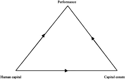
CON=γ0+γ1x1+ · · · +γJxJ+γEEDU+θ2z2+ω, (10) whereE(ω)=0, z2 is the identifying instrument(s) for finan-cial constraints and θ2 is its estimated coefficient(s), satisfy-ing the same conditions (a) and (b) of validity and quality as should hold forz1andθ1. Equation (10) also generates an es-timate of the effect of schooling,EDU, on capital constraints, whereEDUis taken to be exogenous in this equation. The the-oretical case for endogeneity ofEDU is weaker in the capital constraint context, because it seems unlikely (although possi-ble) that individuals acquire schooling to bypass capital con-straints that they might encounter in the future. Although the problem of unobserved heterogeneity in both equations is per-haps a more plausible reason, in fact we found no empirical support for this possibility when we tested for it, as we discuss later. This endows the model with the “endogenous triangle”
Figure 1. The Endogenous Triangle.
structure (between human capital, capital constraints, and per-formance) illustrated in Figure 1.
The parameters of the structural performance equation (8) and the reduced forms for EDU and CON can be estimated by 2SLS. This renders consistent estimates of the parameters of interest (namelyβE,βC, andγE), so that the three propositions of Section 2 can be tested. In short, Propositions 1–3 suggest the parameter restrictionsβC<0,γE0, andβE>0, withγE<0 under the separability assumption discussed earlier.
4. DATA
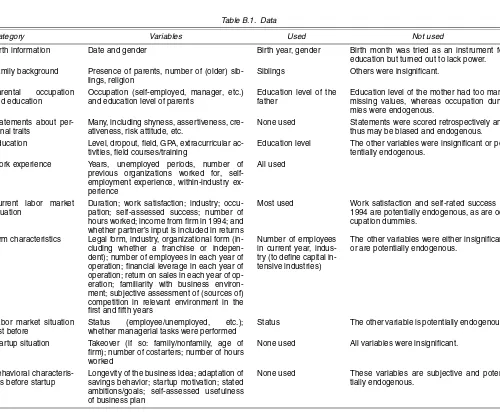
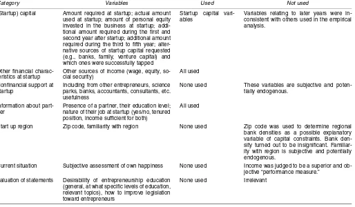
The dataset used in our empirical application is a random cross-sectional sample of Dutch entrepreneurs. Entrepreneurs were defined as individuals who started their own business from scratch or who took over an existing business. Therefore, our focus is on individuals who start up rather than firms that do so. The sample was generated as part of a public–private joint venture executed by the University of Amsterdam, the Erasmus University of Rotterdam, and the GfK market research com-pany. It was commissioned by RABO, a large Dutch cooper-ative bank, and the General Advisory Council of the Dutch Government. The dataset contains a wide range of economic and demographic variables, including ones relating to human capital, financial capital, and business performance. A unique aspect of the dataset is its detailed coverage of startup finance information, necessary for the construction of a continuous cap-ital constraint variable, together with personal characteristics of the entrepreneur dated back to the time of startup and ear-lier. A data appendix (App. B) provides additional details about variables contained in the dataset.
In Fall 1994, a questionnaire was sent to 1,069 entrepre-neurs who had already indicated their willingness to par-ticipate in the research. Of these, 709 responded. Of these, 125 respondents did not provide sufficient information to con-struct a measure of capital constraints, and of the remaining 584 respondents, 123 did not provide information about their income. That left 461 valid observations (including 1 female outlier, subsequently deleted, whose startup capital was more than 15 standard deviations larger than the mean) that were compiled in 1995. As documented by Brouwer, Edelmann, van Praag, and van Praag (1996), the sample is broadly represen-tative of the Dutch population of entrepreneurs in terms of in-dustry, company size, legal form, and age of companies and
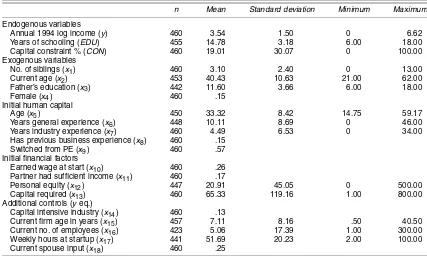
entrepreneurs. The sample contains a slightly larger proportion of highly educated respondents than is found in the general Dutch population, reflecting the fact that one of the commis-sioners of the research project (the General Advisory Council of the Dutch government) was particularly interested in the de-terminants of performance and capital constraints among highly educated individuals. We could not check whether our sample is representative in terms of average business income. But be-cause this variable is so definition-specific (see next section), there is no reason to suppose that entrepreneurs who benefit more from an additional year of schooling will be any more in-clined to respond than are entrepreneurs who benefit less from a marginal year of schooling. Summary statistics of the sample are given in Table 1.
To clearly define our measures of entrepreneurial perfor-mance, human capital, and financial constraints—and also to provide explicit linkage between the theoretical analysis and empirical specification—we next describe the key variables of interest. We give particular attention to the constraint variable, which we believe is a novel one that improves on other mea-sures used in the literature to date.
4.1 Endogenous Variables
Entrepreneurial performance (y) is measured as the natural log of 1 plus total gross annual business profits from the venture in 1994 Dutch guilders (1.85 guilders=1 U.S. dollar in 1994). Gross business profit is defined as all income from the business before deducting tax and social security contributions but after deducting business-related costs. Hence this variable approxi-mates profits rather than revenues, consistent with the discus-sion in Section 2; responses were obtained from one composite question in the survey questionnaire. Every respondent was as-sured of anonymity by the survey interviewers, although it is possible that some income underreporting still occurred. The results will not be affected by idiosyncratic underreporting un-less underreporting behavior varies systematically with educa-tion and/or capital constraints, and any measurement errors that render values of y“noisy” will leave our estimates unbiased, although they would increase their standard errors. For those running businesses jointly with their spouse, joint income was reported; we control for this by including a dummy variable for input into the business by a spouse or partner.
Income from businesses, including wages paid to entre-preneurs as well as returns to capital, is measured compre-hensively. In an attempt to control for returns to capital, all performance regressions include controls for capital required and personal equity invested in the business. (We also tried including controls for whether the business was incorporated, because incorporated firms pay their directors an “employee” wage, but this proved to be insignificant.) An advantage of us-ing log profit as a measure of performance is that it facilitates a comparison of the returns to education from the literature on employee earnings functions.
Unfortunately, the sample surveyors converted any negative profits to zero. There were 28 cases with 0’s, which include “genuine” 0’s as well as converted cases. All of these are in-cluded in the sample because y is defined as ln(1+profit). Clearly, this treatment of negative profits biases average mea-sured performance above the “true” level. However, an attempt
Table 1. Summary Statistics of the Variables Used in the Model
n Mean Standard deviation Minimum Maximum
Endogenous variables
Annual 1994 log income (y) 460 3.54 1.50 0 6.62
Years of schooling (EDU) 455 14.78 3.18 6.00 18.00
Capital constraint % (CON) 460 19.01 30.07 0 100.00
Exogenous variables
No. of siblings (x1) 460 3.10 2.40 0 13.00
Current age (x2) 453 40.43 10.63 21.00 62.00
Father’s education (x3) 442 11.60 3.66 6.00 18.00
Female (x4) 460 .15
Initial human capital
Age (x5) 450 33.32 8.42 14.75 59.17
Years general experience (x6) 448 10.11 8.69 0 46.00
Years industry experience (x7) 460 4.49 6.53 0 34.00
Has previous business experience (x8) 460 .15
Switched from PE (x9) 460 .57
Initial financial factors
Earned wage at start (x10) 460 .26
Partner had sufficient income (x11) 460 .17
Personal equity (x12) 447 20.91 45.05 0 500.00
Capital required (x13) 460 65.33 119.16 1.00 800.00
Additional controls (yeq.)
Capital intensive industry (x14) 460 .13
Current firm age in years (x15) 457 7.11 8.16 .50 40.50
Current no. of employees (x16) 423 5.06 17.39 1.00 300.00
Weekly hours at startup (x17) 441 51.69 20.23 2.00 100.00
Current spouse input (x18) 460 .25
NOTE: Standard deviations, minimum values, and maximum values are omitted for dummy variables.Nis the number of valid observations. This can be less than 460 because nonresponses or missing observations vary according to the question asked. Income is measured in thousands of Dutch guilders in 1994 prices, with mean 70.45 (standard deviation=79.32). PE is paid employment. For the detailed definition of variables, see the text.
to deal with this using a tobit estimator suggests that it probably has little impact on our results. Estimating performance mod-els by tobit changed the constant term slightly, but otherwise the coefficient estimates were more or less unchanged, includ-ing the return to education (we do not report these results for brevity). Perhaps more important, however, is the possibility that the small number of negative incomes implies overrepre-sentation in our sample of “successful” entrepreneurs. To the extent that is true, our results below should be treated with req-uisite caution.
The second endogenous variable is human capital,EDU. The aspect of human capital that we focus on here is education. It was felt that trying to endogenize additional dimensions of human capital, such as years of experience, would entail too many theoretical and empirical complexities, which go beyond the scope of this article. We measure education as the number of years of schooling rather than the highest schooling level at-tained.
The third endogenous variable is capital constraints,CON. This is a more broadly defined variable than borrowing con-straints because, unlike the latter, it also takes into account the possibility that some individuals use their own personal equity to fund their startups, either in part or in whole. The theoretical analysis in Section 2 abstracted from this issue. In fact, per-sonal equity is widespread in our sample; 81% of respondents injected at least 1,000 guilders of their own savings into their business at the time of startup, and 66% injected at least 3,000 guilders.
The theoretical model is easily extended to deal with per-sonal equity. Reflecting banking practice in the Netherlands (and many other countries), an entrepreneur first declares to the lender his of her initial investment of personal equity in the business, denoted byA, and requests the desired amount of
bor-rowingk∗givenA. As the next step, the lender conditions the loan on the basis of the available information (includingA) and offerske. All entrepreneurs with the same personal equity and observable characteristics should experience the same type I ra-tioning, withk∗>kefor the reasons given before.
To construct a measure of capital constraints, we take note of two issues: multiple lenders and the need to control for personal equity as a source of finance, which might dilute borrowing constraints. First, we measureketo allow for loans from possi-bly multiple lenders. Our data on capital borrowed from lenders is not restricted to bank borrowing (although we counted only business loans, not consumer loans). To be consistent with the theoretical analysis, which applies to any kind of borrowing, we used sample data on several finance sources, including banks, venture capitalists, government loan agencies, and trade credit, to compute the total amount borrowed. Of these, banks were the most commonly used source of finance, by one-third of all respondents in the sample. Second, defineKeandK∗as the to-tal amounts of capito-tal used and required (rather than borrowed), whereKe=A+keandK∗=A+k∗. In particular, values ofK∗ were given as responses to the questionnaire question “How much capital did you need at the start of your current busi-ness?” and those ofKeas responses to the question “What was the amount of money that you actually started with?” It was clear from the survey question that loans were for business pur-poses rather than for personal consumption use. Values of A were given as responses to the question “How much of your own money did you invest in the company at the start?”
Now, analogous to (5), the extent to which an individual is capital-constrainedcan be measured as
:=1−K
e
K∗ =1− ke+A
k∗+A∈ [0,1]. (11)
Because every term in (11) is measurable, forms the basis of our empirical measure of capital constraints. As can be seen by differentiating and δ with respect to ke andk∗, has the same properties asδ, in the sense that the relevant proposi-tions of the previous section (i.e., Props. 1 and 2) continue to apply. Note, however, that because∂/∂A<0 and given that A≥0 by definition, it follows that≤δ. This implies a weaker (empirical) relationship between performance and capital con-straints than between performance and borrowing concon-straints in Proposition 1.
In our empirical work we work with the scaled capital con-straint variable CON:=100. Arguably, CON captures the notion of constraints more precisely than do measures of fi-nancial capital, such as savings, assets, inheritances, and lottery outcomes, used in many previous studies. Previous empirical research suggests a positive relationship between financial cap-italand entrepreneurial entry and performance (e.g., Evans and Jovanovic 1989; Holtz-Eakin et al. 1994). But these studies do not measure capital requirements, so such a relationship is not necessarily indicative of capital constraints. For example, the observed empirical relationship might simply reflect decreasing absolute risk aversion (Cressy 2000), or a positive competition externality (Black, de Meza, and Jeffreys 1996). Furthermore, recent research (Hochguertel 2003; Hurst and Lusardi 2004) casts doubt on the robustness of this relationship.
Another advantage ofCONis that it is a continuous variable. Thus in general it will have greater information content than dummy variables (used by, e.g., Astebro and Bernhardt 2003) that indicate whether an entrepreneur believes herself or himself to be credit-constrained.
One drawback of CON is that it is based on self-reported data. Individuals might give biased estimates of their required and actual initial capital values (a problem that might also be shared by some previous empirical studies using self-reported asset values). On the other hand, entrepreneurs might exagger-ate capital requirements when approaching lenders as a negoti-ating tactic. If so, then at least it seems plausible that responses obtained from an anonymous questionnaire, as in the sample used here, could be more accurate than those obtained from bank file data.
Finally, it is worth pointing out that the institutional frame-work in the Netherlands corresponds to that assumed in the the-ory in two important respects. First, personal equity is indeed usually contracted with the bank upfront in the Netherlands, as we assumed. Second, once creditors have exercised their claims on a bankrupt’s assets, the latter faces no future income garnish-ing, so entrepreneurs do indeed face a personal lower bound of zero net wealth [see, e.g., (1)].
4.2 Instruments and Control Variables
The endogenous variables not only are related to each other, as already discussed, but also may depend on exogenous vari-ables. The identifying instruments used in the schooling equa-tion (9) are the respondent’s father’s educaequa-tion (measured as years of schooling) and the number of siblings in the re-spondent’s family. These are common, although not undis-puted, choices in the returns to schooling literature (see, e.g., Blackburn and Neumark 1993, 1995). Although some other au-thors (e.g., Harmon and Walker 1995; Acemoglu and Angrist
1999) have sought identification in terms of regional and le-gal variations in education, these sources of variation are them-selves not immune to criticism (Card 2001) and are in any case unavailable in the Netherlands. Therefore, we proceed cau-tiously using our instruments, which we discuss further later. We supplement these with controls for current age and its square (capturing possible cohort effects) and gender.
Finding valid identifying instruments for the capital con-straint equation (10) requires isolating variables that affect these constraints without directly affecting performance. Recall that the model hypothesized screening errors as the principal rea-son for a relationship between performance and capital con-straints. It seems plausible that bank screening errors, and hence the incidence of capital constraints, will be greater in more capital-intensive industries in which production processes are more complex and the amount of intangible capital also may be greater. Evidence from investments in computers, for example, indicates strong complementarity between tan-gible and intantan-gible investment (Brynjolfsson and Yang 1999; Brynjolfsson and Hitt 2003). This, in a similar vein to the work of Hurst and Lusardi (2004), we propose as an identifying in-strument an indicator variable for whether or not the industry is intensive. Note that there is no requirement that capital-intensiveness affects performance.
We define the following industries as capital-intensive: man-ufacturing (including production and construction) and trans-portation (including storage). These industries had the highest ratio of fixed assets to wage costs (our measure of capital-intensiveness) in 1994 according to Dutch Bureau of Statis-tics (CBS) data. Manufacturing and transportation both ranked equal highest with a ratio of 3.3. Together, their share of fixed assets amounts to 64.6%, whereas their share of employees amounts to 34.9%. These industries compose 13% of our sam-ple (Table 1). The other 87% of the firms in our dataset are in the following industries: retail and wholesale trade (including restaurants, hotels, and pubs), services (professional, financial, and “other”), repair, agriculture, recreation, education and re-search, health and social care, and agriculture. The capital in-tensity of these other industries ranged from 1.1 (professional services) to 2.4 (agriculture).
The other variables used in the capital constraint and per-formance equations include (endogenous) years of schooling, gender, and several exogenousinitial human capitalvariables. The latter set of variables includes number of years of work experience (both general and in the same industry), whether the entrepreneur had previous business experience, and whether the entrepreneur switched from paid employment (PE, in the public or private sector) just before to startup. We expect all of these variables to be positively associated with subsequent perfor-mance (because human capital is valuable) and negatively as-sociated with capital constraints—for example, because lenders use them as favorable indicators of ability and creditworthiness (see Sec. 2.2).
Performance and capital constraints might also be affected by entrepreneurs’initial financialcircumstances. For example, consider an entrepreneur who continued to receive some wage income at the time of startup or who had a spouse or partner who earned sufficient income at that time for the venture to sur-vive poor performance. Such “external” (i.e., nonentrepreneur-ial) income sources can be expected to relax an entrepreneur’s
capital constraint. Their effects on performance might go either way, however. On the one hand, by decreasing the variability of household resources, extra income sources might permit the entrepreneur to choose a project occupying a higher point on the risk–return trade-off. On the other hand, extra sources of in-come might distract the entrepreneur’s attention from running the core business. In the case of additional income from wages, the entrepreneur is presumably diverting some effort directly from the business to paid employment. In the case of having a working spouse, the entrepreneur might be required to con-tribute more time to household production, and so less to the business, than would otherwise be the case.
From (11), the extent of capital constraints is a decreasing function of initial personal equity,A, and an increasing func-tion of total capital required,K∗. But both variables might have additional effects by also affecting the capital obtained from lenders. For example, lenders frequently value injections of personal equity as collateral, because this can make an entire loan relatively safe from their perspective. The opposite is the case with regard to the size of the loan itself. To avoid compli-cations caused by (arbitrary) specificompli-cations of nonlinear func-tional forms, but to nonetheless capture the main idea, we enter these two variables (which are measured at the time of startup) in the capital constraint and performance equations in both lev-els and squares.
Other control variables that are likely to affect entrepreneurs’ current performance—but not their historical education deci-sion and initial capital constraints—include the current age of the firm current firm size (measured by the number of full-time equivalent employees, including the entrepreneur himself or herself ), and the average weekly number of hours worked in the first year of the venture.
5. RESULTS
This section is divided into four parts. In the first part we demonstrate the importance of treating years of schooling and capital constraints as endogenous variables. We also obtain em-pirical backing for the “endogenous triangle” structure of our model and evaluate our choice of instruments. In the remaining parts we present and interpret the schooling, capital constraint, and performance equations.
5.1 Importance of Endogeneity Issues
It has been suggested that both years of schooling and capi-tal constraints are likely to be endogenous variables in the en-trepreneurial performance equation, whereas schooling is less
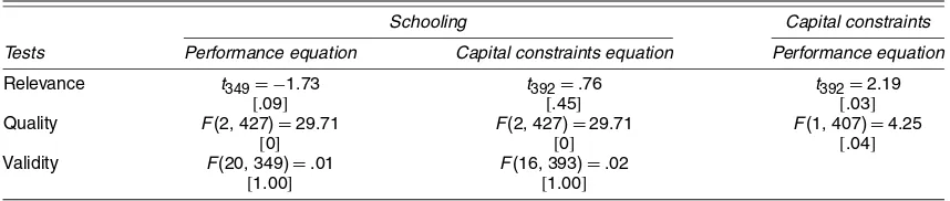
likely to be endogenous in the capital constraint equation. We can test directly the relevance of correcting for endogeneity in each of these three cases by applying Hausman’s (1978) ttest. The validity of Hausman’s test depends on the underlying choice of identifying instruments satisfying quality and validity criteria, tests of which we also provide.
Row 1 of Table 2 presents the Hausman tests for endo-geneity. The significance of the statistics given in the first and third columns suggests that years of schooling and capital con-straints are indeed endogenous in the entrepreneurial perfor-mance equation. The insignificance of the statistic in the second column implies that years of schooling can indeed be treated as exogenous in the capital constraint equation, justifying the tri-angular structure of our model.
We now test whether the proposed identifying instruments are of high quality and are also valid. Following Bound, Jaeger, and Baker (1995), the quality of the instrument set can be gauged byFstatistics that test the null hypothesis of insignif-icant instrumentsθ1 andθ2in (9) and (10). Row 2 of Table 2 presents the test statistics for the quality of the identifying in-struments for years of schooling (9) and capital constraints (10); columns 1 and 2 are identical because they both relate to (9). The significance of these “partialF” statistics suggests that the proposed identifying instruments are indeed of high quality in both cases.
Instruments are valid if they affect performance through the instrument equation (9) or (10) only. Sargan’s F statistic (Davidson and MacKinnon 1993) tests the null hypothesis that the identifying instruments are orthogonal to the error of the IV equation. But Sargan’s test can be performed only if more than one identifying instrument is used. Therefore, unfortu-nately, the validity of the instrument “capital intensity” pro-posed for the capital constraint equation cannot be tested. This explains the blank cell in the last row and column of Table 2. The first two columns of row 3 of Table 2 show that the instru-ments proposed for the schooling decision are indeed valid for equations (9) and (10) according to Sargan’sFstatistic. The re-sult for years of schooling vis-à-vis the performance equation is especially reassuring, because it counters the criticism that family background variables might be invalid instruments be-cause they are correlated with unobserved ability and thereby affect entrepreneurs’ performance (see Card 1999, 2001 for a discussion).
5.2 Explaining the Schooling Decision
The first column of Table 3 presents estimates of the school-ing equation (9). Both this equation and the capital constraints
Table 2. Diagnostic Tests of Instrument Relevance, Quality, and Validity
Schooling Capital constraints
Tests Performance equation Capital constraints equation Performance equation
Relevance t349= −1.73 t392=.76 t392=2.19
[.09] [.45] [.03]
Quality F(2, 427)=29.71 F(2, 427)=29.71 F(1, 407)=4.25
[0] [0] [.04]
Validity F(20, 349)=.01 F(16, 393)=.02
[1.00] [1.00]
NOTE: Each cell gives the diagnostic test result withpvalues in square brackets. The “relevance,” “quality,” and “validity” tests are defined in the text.
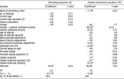
Table 3. Estimates of the Schooling and Capital Constraint Equations
Schooling equation (9) Capital constraints equation (10)
Variable Coefficient t-ratio Coefficient t-ratio
Years of schooling,EDU −1.18∗ 2.20
No. of siblings −.18† 2.71
Current age .29∗ 2.50
Current age squared/10 −.04† 3.15
Father’s education .28† 7.42
Female −.78∗ 2.25 −.84 .17
Female×partner sufficient income −18.03∗ 2.15
Partner sufficient income 8.78 1.77
Age at startup .29 .23
Age at startup squared −.01 .38
Years general experience .22 .68
Years industry experience −.39 1.60
Has previous business experience 5.44 1.29
Switched from PE −9.36† 3.00
Earned wage at start .95 .29
Personal equity −.34† 5.03
Personal equity squared/10 .01† 3.88
Capital required .14† 3.32
Capital required squared/100 −.01† 2.96
Capital intensive industry 8.72∗ 2.06
Intercept 8.22† 3.54 36.65 1.54
R2 .31 .13
F(k,n−k) 41.74† 4.98†
No. of observations,n 433 424
NOTE: Dependent variables are defined in the text. Regressions are reported with robust standard errors.kis the number of parameters, andn−kis the degrees of freedom. The sample size reduces to 433 in the schooling equation because of the 460 initial observations, 7, 5, and 15 observations were missing for “age,” “years of education,” and “father’s education.” The sample size is 424 in the capital constraints equation because of missing data on these and some additional explanatory variables (precise details are available on request).
†p<.05.
∗p<.01.
equation discussed shortly contain a mixture of identifying in-struments and controls for which the values were known at the time the schooling decision was made [see (9)] and at the time the business was started up [see (10)]. Both of the identify-ing instruments “number of siblidentify-ings” and “father’s education” are statistically significant determinants of years of education, and the regression as a whole is also significant [F(6,428)=
41.74]. Individuals born in families whose fathers are better educated and there are fewer siblings to compete for attention and resources tend to acquire significantly more education than average. Of the two identifying instruments, father’s education is the more powerful; whereas the results were unchanged by dropping the number of siblings, the predictive power of the number of siblings on its own was too low to precisely estimate the effect of schooling on performance. We also tried alternative identifying instruments based on religious affiliation of schools and the birth month of the respondent, but neither of these vari-ables was statistically significant. Therefore we, proceed using both identifying instruments.
Our findings are similar to those of Van der Sluis et al. (2004) for entrepreneurs and of Blackburn and Neumark (1993) and Levin and Plug (1999) for employees. We also find that females obtain significantly less education than average, and there also seems to be a cohort effect at work, whereby older respondents obtained more education than younger respondents. Overall, the respectable fit attained by this regression (R2=.31) suggests that it forms a reasonable basis for estimating the impact of education on entrepreneurial performance. We do, however, ac-knowledge the limitations of the available instruments used in this regression.
5.3 Explaining the Extent of Entrepreneurs’ Capital Constraints
The final column of Table 3 presents estimates of the capi-tal constraint equation (10). The key result is that extra years of schooling significantly decreases capital constraints. The es-timated coefficient is large in absolute terms and statistically significant with ap value of 2.8%. This result, which implies that an extra year of schooling relaxes the capital constraint by 1.18%, is consistent with Proposition 2 (and separable entrepre-neurial production functions). It implies that lenders are more willing to provide funds to better-educated entrepreneurs, all else being equal.
In addition, we find that entrepreneurs located in capital-intensive industries are significantly more likely to face capital constraints than those located in industries in which less cap-ital is needed. This effect is additional to a scale effect from required capital and so is consistent with a theoretical argu-ment that banks’ screening errors are systematically greater in some industries in which more complicated production tech-niques with complementary intangible capital are used.
It is also of interest to interpret other coefficients in Table 3. Women whose partners had sufficient income to support the household at the time of startup face lower capital constraints, presumably because they can obtain resources from their part-ners. A similar mechanism was not observed for men. This was the only significant difference in capital constraints by gender; gender interactions with the other variables failed to achieve significance. Another characteristic that appears to mit-igate capital constraints is having switched into
ship from paid employment just before startup. Such behavior might serve as a positive signal to lenders, thereby encouraging them to offer more financing. As expected, the amount of per-sonal equity injected at the start has a strongly negative and non-linear effect on the extent of capital constraints. The absolute size of this effect decreases as the amount of personal business capital increases. The effect of the total amount of capital re-quired by an entrepreneur on the extent of capital constraints is significantly positive and also has a decreasing marginal effect. This might reflect lenders’ unwillingness to overextend them-selves on risky investment projects. More than 97% of respon-dents have net negative effects from personal equity and net positive effects from capital required.
All of the other variables in Table 3 are statistically insignif-icant. TheR2of 13% indicates that we have had only limited success in explaining the extent of capital constraints, which is consistent with our earlier assumptions of unobserved abil-ity and lender screening errors that underlies Proposition 1. No doubt this result might also provide encouragement to those who argue that many bank decisions on offering startup fi-nance are arbitrary, based predominantly on such intangible factors as “first impressions” and prejudice rather than on tan-gible observable characteristics. Indeed, our dataset contains detailed personal and financial information that encompasses what is typically found in bank file data (cf. Cressy 1993); and checks confirm that none of these extra variables (e.g., the le-gal form and structure of the startup and familiarity with the business environment) were significant in the capital constraint
equation. We also found no evidence that entrepreneurs with greater collateral other than personal equity faced lower cap-ital constraints. Although the dataset contains no information on collateral directly, it does contains responses to two related questions: whether individuals raised finance by releasing eq-uity from their houses, and whether they took over their firm (in which case they may have tangible collateral in place) or started it from scratch. Neither variable significantly decreased capital constraints. In addition, neither an indicator variable of whether entrepreneurs took over a firm from family members nor a dummy variable indicating access to loans at subsidized rates was significant. The latter included funds obtained from family, friends, government program, and business partners. Detailed results are available on request.
5.4 Explaining Entrepreneurs’ Performance
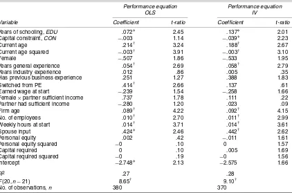
We now present results from estimating equation (8), that is, the determinants of entrepreneurs’ performance. We present re-sults, summarized in Table 4, using both OLS and IV estima-tors. We discuss how this comparison underlines the practical importance of correcting for endogeneity biases when attempt-ing to explain entrepreneurs’ performance.
5.4.1 Entrepreneurs’ Returns to Schooling. The first col-umn of Table 4 shows the (biased) estimation results that ensue when estimating (8) by OLS. It reports an average rate of return to schooling of 7.2%, supporting Proposition 3. A comparison with other OLS estimates of the return to schooling in entre-preneurship reveals that this estimate is a little higher than, but
Table 4. Estimates of the Enterprise Performance Equation
Performance equation Performance equation
OLS IV
Variable Coefficient t-ratio Coefficient t-ratio
Years of schooling,EDU .072∗ 2.45 .137∗ 2.01
Capital constraint,CON −.003 1.14 −.039∗ 2.23
Current age .214† 3.24 .188† 2.67
Current age squared −.003† 3.91 −.003† 3.10
Female −.507 1.86 −.533 1.95
Years general experience .054† 2.69 .058† 2.79
Years industry experience .012 .86 .005 .35
Has previous business experience .251 1.27 .388 1.83
Switched from PE .414† 2.66 .137 .61
Earned wage at start −.239 1.54 −.258 1.66
Female×partner sufficient income .737 1.78 .111 .22
Partner had sufficient income −.280 1.20 .023 .09
Firm age .089† 4.22 .092† 4.15
No. of employees .010† 2.70 .011† 2.99
Weekly hours at start .014† 3.71 .014† 3.61
Spouse input .424∗ 2.46 .442† 2.62
Personal equity .002 .42 −.011 1.61
Personal equity squared −0 .10 0 1.57
Capital required 0 .10 .005 1.69
Capital required squared −0 .19 −0 1.56
Intercept −2.748∗ 2.13 −2.575 1.66
R2 .27 .28
F(20,n−21) 8.65† 9.10†
No. of observations,n 380 370
NOTE: Dependent variables are defined in the text. Regressions are reported with robust standard errors. Method of estimation is given at the head of the table. The sample size reduces to 370 for the IV results because of the 424 observations used in the capital constraint instrumented equation, 33, 11, and 10 observations were missing for “no. of employees,” “weekly hours at start,” and “father’s education.” It is 380 for OLS because the absence of instrumentation avoided the need to discard 10 of these observations.
∗p<.05.
†p<.01.
broadly comparable with, previous findings. For example, in a survey of 21 previous studies of the relationship between edu-cation and entrepreneurial earnings, Van der Sluis et al. (2003) reported an average rate of return of 6.1% for studies based on U.S. data, with a somewhat lower average rate of return for Eu-ropean studies.
The second column of Table 4 presents the results using IV estimation. Like previous comparisons between IV and OLS conducted for employees, the IV estimate is substantially higher than the OLS estimate, 13.7% versus 7.2%. For exam-ple, the average IV estimates of Ashenfelter et al. (1999) were nearly 3% higher than their OLS estimates, whereas Harmon and Walker (1995) and Lemieux and Card (1998) reported even larger differences between IV and OLS. Our IV estimate, which remains statistically significant, is somewhat higher than IV estimates for employees in similar countries. For example, Ashenfelter et al. (1999) reported an average IV rate of return for employees of 9.3%.
Such comparisons are of intrinsic interest for at least two rea-sons. First, they might carry policy implications for programs designed to encourage high school and college graduates to become entrepreneurs. In the case of the foregoing estimates, for example, they might help justify public expenditure on such programs, especially if the social and private returns to educa-tion are higher for entrepreneurs than for employees. Of course, this interpretation is subject to the earlier caveat that our results are only as good as the instruments on which they rely, and in the case of years of schooling in particular, these are not beyond reproach.
Second, entrepreneurs’ rate of return to education bears on a long-standing question about whether rates of return to school-ing for employees contain a signalschool-ing component (Wolpin 1977). For example, it is sometimes argued that because only employees need to signal abilities to employers, they will earn higher average returns on their investment than entrepreneurs if the marginal productive effects of their education pursued are equal (Riley 1979, 2002). In addition, entrepreneurial success is likely to depend on numerous factors other than formal ed-ucation, again implying that entrepreneurs will obtain a lower return to schooling than employees. On the other hand, entre-preneurs might invest in education as a hedge or to work for others before commencing a spell in entrepreneurship, and cus-tomers, suppliers of credit, and government agencies might also screen entrepreneurs, especially in those industries in which the incidence of self-employment has grown rapidly in recent years, such as professional services. The available evidence cer-tainly does not support the notion that entrepreneurs receive lower returns to education than wage employees do; however, we are unable to shed any more light directly on this issue be-cause our dataset is limited to entrepreneurs. Instead, we ex-plore whether the indirect effect of education on performance, through its impact on capital constraints, further increases the total impact of years of schooling on entrepreneurs’ business incomes.
5.4.2 The Role of Capital Constraints. The first column of Table 4 shows that the (biased) estimate of the effect of capital constraints on entrepreneurs’ business incomes is nu-merically small and statistically insignificant. However, the IV estimate given in the second column is more than 10 times
larger and is highly significant. It implies that a 1 percentage point relaxation of capital constraints increases entrepreneurs’ average business incomes by 3.9%. This finding strongly sup-ports Proposition 1.
The size of this effect appears substantial, although it should be borne in mind that the average extent of capital constraints faced by entrepreneurs in our sample is only 19%. Hence, if the capital constraints of an entrepreneur with average capital constraints are alleviated by 10% (i.e., 1.9 percentage points), then the resulting income change is.039×1.9=7.4%. We em-phasize that the estimated effect of capital constraints on per-formance is obtained after controlling for personal equity and capital required, the inclusion of which had little overall effect. Next, we measure the indirect effect of schooling on perfor-mance through the capital constraint. Using (10) and (8), this can be estimated as βˆCγˆE=.039×1.183=.046. This sug-gests a total rate of return from schooling for entrepreneurs of 18.3%. A different estimate of the indirect effect can be ob-tained by reestimating (8) but excluding the capital constraint variable. This will give a lower estimate, because omitting cap-ital constraints causes downward bias in thecombined return to education. The total return to schooling is then estimated as 16.7% (t-statistic=2.48;p=.013). Thus the implied indirect effect according to this estimate is 3%. Nevertheless, the range of 3.0–4.6% further underscores the importance of human cap-ital for entrepreneurial success.
5.4.3 Effects From Control Variables. We also find some interesting effects from some of the other control variables in Table 4. Work effort, measured in terms of hours worked by the entrepreneur and having a spouse work input in the busi-ness, and human capital, as measured by age and general ex-perience, are two important sets of variables that significantly and substantially enhance entrepreneurs’ performance. By rep-resenting basic determinants of entrepreneurs’ marginal pro-ductivity, their significance might not appear too surprising. But the nature of productive experience is particularly note-worthy. Several authors have previously distinguished between experience gained in business and experience gained in paid employment (see, e.g., Evans and Leighton 1989a). Here we find that the rate of return to an extra year of general experi-ence is statistically significant, 5.8% on average. This includes previous experience in business and in the same industry, as well as experience gained elsewhere. But no additional signif-icant effects from business and same-industry experience were found when they were entered separately. Moreover, consistent with a large body of empirical work, the relationship between performance and age is positive and concave (see also Brock and Evans 1986; Evans and Leighton 1989b; Holtz-Eakin et al. 1994).
The remaining control variables also have the expected ef-fects on performance. Entrepreneurs’ log incomes are higher on average for older and larger (in employment terms) businesses. These findings are consistent with Jovanovic’s (1982) theory of industry evolution, reflecting survival by both the most able and also the most knowledgeable about their innate abilities in entrepreneurship. Finally, female entrepreneurs earn lower log incomes on average than their male counterparts. But this ef-fect, which is attenuated for females with richer spouses, is on the margins of statistical significance.
5.4.4 Sensitivity Analysis. We conducted several robust-ness checks to see whether our results are sensitive to different specifications or are consistent with alternative explanations. One alternative explanation for the substantial effect of educa-tion on performance is that more educated entrepreneurs choose to operate risky projects with high rates of return. As Cocco, Gomes, and Maenhout (2005) and Gomes and Michaelides (2005) have pointed out, human capital is less risky than eq-uities and so can substitute for bond holdings, enabling riskier nonhuman capital investments. Hence higher levels of educa-tion might increase average performance by making the value of the human capital hedge greater (Polkovnichenko 2003). To check for this, we split the sample into different groups by year of education and for each group computed the coefficient of variation in incomes as a measure of education-specific income uncertainty. If education were acting as a hedge in this way, then we would expect the coefficient of variation to be related positively to years of schooling. In fact, however, we found a negative correlation between the coefficient of variation and schooling (−.0506), although this was insignificant (thep-value was .9053). On its face, this suggests that our results seem to be robust to hedging properties of human capital. However, as a referee pointed out, our dataset may be susceptible to a sur-vivorship bias that is especially pronounced for the riskier busi-nesses, and we do not have data on thesystematiccomponent of entrepreneurial returns, for which time series data are needed. Thus we are forced to accept that our results do not conclu-sively rule out the possibility that more educated entrepreneurs undertake riskier projects.
It is also possible that rates of return to education depend on such milestones as completing high school or college. To test this, we included and interacted dummies for completion of high school and college education with years of education in the performance equation. None of these additional terms was statistically significant. For example, a dummy variable indi-cating college dropout and its interaction with years of educa-tion achievedpvalues of only .386 and .209 in the performance equation. This suggests that our estimated rates of return are correctly capturing the effects of education on performance.
Another possibility is that individuals at different wealth lev-els face qualitatively different constraints. This possibility is suggested by the findings of Hurst and Lusardi (2004), who re-ported that assets affect participation in entrepreneurship only for those at the top end of the wealth distribution. To test this possibility, we defined a dummy variable, “top,” as equal to 1 if the respondent appeared in the top quintile of the asset distrib-ution. Personal equity was used as a proxy for net wealth, be-cause the latter was unavailable in our dataset. This dummy was interacted with every variable in the capital constraint equation. The intercept dummy was−6.263 (t-statistic=1.65,p=.099), and none of the other coefficients was statistically significant. This suggests that whereas wealth decreases capital constraints, it does not change the relationship between capital constraints and its other determinants. However, it should be borne in mind that we are using only a proxy for wealth and are analyzing a sample of individuals who are already participating in entrepre-neurship.
Next, we checked whether the results change when the sam-ple is restricted to younger entrepreneurs (say, younger than
30 or 40 at the start). As an anonymous referee pointed out, younger entrepreneurs might have less wealth and so may face greater capital constraints. In fact, restricting the sample in this way yielded results that were qualitatively the same as for the entire sample, although some of the relationships lacked sig-nificance because of the small resulting sample size. Moreover, including a dummy variable that differentiated younger entre-preneurs from older ones in the capital constraint and perfor-mance equations yielded no significant results. These findings bear out the results in Table 3 demonstrating that capital con-straints do not seem to vary significantly with age.
Finally, we explored several other possible identifying instru-ments for capital constraints. One of the referees asked whether variations in regional bank densities in the Netherlands might represent a useful instrument. The idea is that entrepreneurs in areas of high bank density would find it easier to undergo repeated screening by rival banks if they were given unfavor-able initial loan offers. The data on number of banks per zip code area were collected from www.bedrijven.nl and entered into the capital constraints equation as an additional instrument. But this instrument lacked power, having a partial F statistic of only .004. We also tried several other candidates, including whether the business was taken over (from within or outside the family) as opposed to having been started from scratch. Capital requirements might be easier to screen if the firm already had some trading history, especially for older firms. But none of the alternative candidates for identifying instruments in the capital constraints equation had sufficient power either.
6. CONCLUSION
In this study we investigated the extent to which the per-formance of a business venture, once started, is affected by capital constraints at the time of inception and by the busi-ness founder’s investment in human capital. We attempted to answer this question by measuring the distinct contribution of each of these factors, taking into account the possibility that hu-man capital might also have an indirect effect on perforhu-mance by facilitating access to financial capital, thus diluting any cap-ital constraint. Toward this end, and in recognition of the likely endogeneity of education and capital constraints, we estimated a “triangular” model of capital constraints, years of schooling, and performance by IV, using a sample of data from a rich sur-vey of entrepreneurs conducted in the Netherlands in 1995.
Our principal findings are threefold. First, lower capital con-straints lead to greater entrepreneurial performance, with a 1 percentage point relaxation of capital constraints increasing entrepreneurs’ profits by 3.9% on average. This estimate is both statistically significant and fairly sizeable in economic terms. Second, more years of education is associated with significantly lower capital constraints. Each year of schooling decreases cap-ital constraints by 1.18 percentage points. Third, extra years of schooling enhances entrepreneurial performance both directly and indirectly through the effect of capital constraints. The di-rect rate of return to schooling is estimated as 13.7%, whereas the total effect, including the indirect effect through the im-pact of education on capital constraints, is estimated as between 16.7% and 18.3%. Our dataset is limited to entrepreneurs, so we cannot compare rates of return for employees and entrepreneurs