Full Terms & Conditions of access and use can be found at
http://www.tandfonline.com/action/journalInformation?journalCode=ubes20
Download by: [Universitas Maritim Raja Ali Haji] Date: 12 January 2016, At: 00:22
Journal of Business & Economic Statistics
ISSN: 0735-0015 (Print) 1537-2707 (Online) Journal homepage: http://www.tandfonline.com/loi/ubes20
Nonparametric Discrete Choice Models With
Unobserved Heterogeneity
Richard A. Briesch, Pradeep K. Chintagunta & Rosa L. Matzkin
To cite this article: Richard A. Briesch, Pradeep K. Chintagunta & Rosa L. Matzkin (2010)
Nonparametric Discrete Choice Models With Unobserved Heterogeneity, Journal of Business & Economic Statistics, 28:2, 291-307, DOI: 10.1198/jbes.2009.07219
To link to this article: http://dx.doi.org/10.1198/jbes.2009.07219
Published online: 01 Jan 2012.
Submit your article to this journal
Article views: 411
View related articles
Nonparametric Discrete Choice Models With
Unobserved Heterogeneity
Richard A. BRIESCH
Cox School of Business, Southern Methodist University, Dallas, TX 75275-0333 (rbriesch@mail.cox.smu.edu)
Pradeep K. CHINTAGUNTA
Booth School of Business, University of Chicago, Chicago, IL 60637 (pradeep.chintagunta@ChicagoBooth.edu)
Rosa L. MATZKIN
Department of Economics, University of California–Los Angeles, Los Angeles, CA 90095 (matzkin@econ.ucla.edu)
In this research, we provide a new method to estimate discrete choice models with unobserved hetero-geneity that can be used with either cross-sectional or panel data. The method imposes nonparametric assumptions on the systematic subutility functions and on the distributions of the unobservable random vectors and the heterogeneity parameter. The estimators are computationally feasible and strongly con-sistent. We provide an empirical application of the estimator to a model of store format choice. The key insights from the empirical application are: (1) consumer response to cost and distance contains interac-tions and nonlinear effects, which implies that a model without these effects tends to bias the estimated elasticities and heterogeneity distribution, and (2) the increase in likelihood for adding nonlinearities is similar to the increase in likelihood for adding heterogeneity, and this increase persists as heterogeneity is included in the model.
KEY WORDS: Discrete choice; Heterogeneity; Nonparametric; Random effects.
1. INTRODUCTION
Since the early work of McFadden (1974) on the develop-ment of the conditional logit model for the econometric analy-sis of choices among a finite number of alternatives, a large number of extensions of the model have been developed. These extensions have spawned streams of literature of their own. One such stream has focused on relaxing the strict parametric struc-ture imposed in the original model. Another stream has con-centrated on relaxing the parameter homogeneity assumption across individuals. This article contributes to both these areas of research. We introduce methods to estimate discrete choice models where all functions and distributions are nonparametric, individuals are allowed to be heterogeneous in their preferences over observable attributes, and the distribution of these prefer-ences is also nonparametric.
As is well known in discrete choice models, each individual possesses a utility for each available alternative, and chooses the one that provides the highest utility. The utility of each al-ternative is the sum of a subutility of observed attributes (the systematic subutility) and an unobservable random term (the random subutility). Manski (1975) developed an econometric model of discrete choice that did not require specification of a parametric structure for the distribution of the unobservable random subutilities. This method was followed by other sim-ilarly semiparametric distribution-free methods developed by Cosslett (1983), Manski (1985), Han (1987), Powell, Stock, and Stoker (1989), Horowitz (1992), Ichimura (1993), Klein and Spady (1993), and Moon (2004), among others. More re-cently, Geweke and Keane (1997) and Hirano (2002), have ap-plied mixing techniques that allow nonparametric estimation of
the error term in Bayesian models. Similarly, Klein and Sher-man (2002) propose a method that allows nonparametric es-timation of the density as well as the parameters for ordered response models. These methods are termed semiparametric because they require a parametric structure for the systematic subutility of the observable characteristics. A second stream of literature has focused on relaxing the parametric assump-tion about the systematic subutility. Matzkin’s (1991) semipara-metric method accomplished this while maintaining a paramet-ric structure for the distribution of the unobservable random subutilities. Matzkin (1992,1993) proposed fully nonparamet-ric methods where neither the systematic subutility nor the dis-tribution of the unobservable random subutility are required to possess parametric structures.
Finally, a third stream of literature has focused on incorpo-rating consumer heterogeneity into choice models.Wansbeek, Wedel, and Meijer (2001) noted the importance of including heterogeneity in choice models to avoid finding weak relation-ships between explanatory variables and choice. However, they also note the difficulty of incorporating heterogeneity into non-parametric and seminon-parametric models. Further, Allenby and Rossi (1999) noted the importance of allowing heterogeneity in choice models to extend into the slope coefficients. Specifica-tions that have allowed for heterogeneous systematic subutili-ties include those of Heckman and Willis (1977), Albright, Ler-man, and Manski (1977), and Hausman and Wise (1978). These
© 2010American Statistical Association Journal of Business & Economic Statistics
April 2010, Vol. 28, No. 2 DOI:10.1198/jbes.2009.07219
291
articles use a particular parametric specification, that is, a spe-cific continuous distribution, to account for the distribution of systematic subutilities across consumers. Heckman and Singer (1984) propose estimating the parameters of the model without imposing a specific continuous distribution for this heterogene-ity distribution. Ichimura and Thompson (1994) have developed an econometric model of discrete choice where the coefficients of the linear subutility have a distribution of unknown form, which can be estimated.
Recent empirical work has relaxed assumptions on the het-erogeneity distributions. Lancaster (1997) allows for nonpara-metric identification of the distribution of the heterogeneity in Bayesian models. Taber (2000) and Park, Sickles, and Simar (2007) apply semiparametric techniques to dynamic models of choice. Briesch, Chintagunta, and Matzkin (2002) allow con-sumer heterogeneity in the parametric part of the choice model while restricting the nonparametric function to be homoge-neous. Dahl (2002) applies nonparametric techniques to tran-sition probabilities and dynamic models. Pinkse, Slade, and Brett(2002) allow for heterogeneity in semiparametric models of aggregate-level choice.
The method that we develop here combines the fully non-parametric methods for estimating discrete choice models (Matzkin1992,1993) with a method that allows us to estimate the distribution of unobserved heterogeneity nonparametrically as well. The unobserved heterogeneity variable is included in the systematic subutility in a nonadditive way (Matzkin1999a, 2003). We provide conditions under which the systematic subu-tility, the distribution of the nonadditive unobserved hetero-geneity variable, and the distribution of the additive unobserved random subutility can all be nonparametrically identified and consistently estimated from individual choice data. The method can be used with either cross-sectional or panel data. These re-sults update Briesch, Chintagunta, and Matzkin (2002).
We apply the proposed methodology to study the drivers of grocery store format choice for a panel of households. There are two main formats that for classifying supermarkets—everyday low price (EDLP) stores or high–low price (Hi–Lo) stores. The former offer fewer promotions of lower “depth” (i.e., magni-tude of discounts) than the latter. The main tradeoff facing con-sumers is that EDLP stores are typically located farther away (longer driving distances) than Hi–Lo stores although their prices, on average, are lower than those at Hi–Lo stores lead-ing to a lower total cost of shopplead-ing “basket” for the consumer. Since the value of time (associated with the driving distance) is heterogeneous across households and little is known about the shape of the utility for driving distance and expenditure, we think that the proposed method is ideally suited to understand-ing the nature of the tradeoff between distance and expenditure facing the consumer. To decrease the well-known dimensional-ity problems associated with relaxing parametric structures, we use a semiparametric version of our model. In particular, only the subutility of distance to the store and cost of refilling in-ventory at the store are nonparametric. We allow this subutility to be heterogeneous across consumers and provide an estima-tor for the subutilities of the different types, the distribution of types, and the additional parameters of the model. Further, we assume that the unobserved component of utility in this appli-cation is distributed according to a type-I extreme value distri-bution.
In the next section we describe the model. Section3states conditions under which the model is identified. In Section 4 we present strongly consistent estimators for the functions and distributions in the model. Section 5 provides computational details. Section6presents the empirical application. Section7 concludes.
2. THE MODEL
As is usual in discrete choice models, we assume that a typ-ical consumer must choose one of a finite number,J, of alter-natives, and he/she chooses the one that maximizes the value of a utility function, which depends on the characteristics of the alternatives and the consumer. Each alternativej is character-ized by a vector,zj, of the observable attributes of the alterna-tives. We will assume thatzj≡(xj,rj), whererj∈Randxj∈RK (K≥1). Each consumer is characterized by a vector,s∈RL, of observable socioeconomic characteristics for the consumer. The utility of a consumer with observable socioeconomic char-acteristics s, for an alternative,j, is given byV∗(j,s,zj, ω)+εj, whereεjandωdenote the values of unobservable random vari-ables. For any given value ofω, and anyj,V∗(j,·, ω)is a real-valued but otherwise unknown function. The dependence ofV∗ onω allows this systematic subutility to be different for dif-ferent consumers, even if the observable exogenous variables are the same for these consumers. We denote the distribution of
ωbyG∗and we denote the distribution of the random vector
ε=(ε1, . . . , εJ)byF∗.
The probability that a consumer with socioeconomic char-acteristicss will choose alternative j when the vector of ob-servable attributes of the alternatives is z ≡(z1, . . . ,zJ) ≡
(x1,r1, . . . ,xJ,rJ)is denoted byp(j|s,z;V∗,F∗,G∗). Hence,
p(j|s,z;V,F,G)=
Pr(j|s,z;ω,V,F)dG(ω),
where Pr(j|s,z;ω,V,F) denotes the probability that a con-sumer with systematic subutility V(·, ω)will choose alternative j, when the distribution ofε is F. By the utility maximization hypothesis,
Pr(j|s,z;ω,V,F)
=Pr{V(j,s,xj,rj, ω)+εj>V(k,s,xk,rk, ω)+εk,∀k=j}
=Pr{εk−εj<V(j,s,xj,rj, ω)−V(k,s,xk,rk, ω),∀k=j}, which depends on the distributionF. In particular, if we letF1∗ denote the distribution of the vector(ε2−ε1, . . . , εJ−ε1), then
Pr(1|s,z;ω,V,F∗)
=F∗1
V(1|s,x1,r1, ω)−V(2|s,x2,r2, ω), . . . ,
V(1|s,x1,r1, ω)−V(J|s,xJ,rJ, ω)
and the probability that the consumer will choose alternative one is then
p(1|s,z;V,F∗,G)
=
Pr(1|s,z;V,F∗,G)dG(ω)
=
F1∗
V(1|s,x1,r1, ω)−V(2|s,x2,r2, ω), . . . , V(1|s,x1,r1, ω)−V(J|s,xJ,rJ, ω)dG(ω).
For anyj, Pr(j|s,z;ω,V,F∗)can be obtained in an analogous way, lettingFj∗denote the distribution of (ε1−εj, . . . , εJ−εj). A particular case of the polychotomous choice model is the bi-nary threshold Crossing model, which has been used in a wide range of applications. This model can be obtained from the polychotomous choice model by lettingJ=2, η=(ε2−ε1) and ∀(s,x2,r2, ω),V(2,s,x2,r2, ω)≡0. In other words, the model can be described by:y∗=V(x,r, ω)−η, with
y=
1, ify∗≥0 0, otherwise,
wherey∗ is unobservable. In this model, F1∗ denotes the dis-tribution of η. Hence, for all x, r, ω,Pr(1|x,r;ω,V∗,F∗)=
F∗1(V∗(x,r, ω))and for allx,rthe probability that the consumer will choose alternative one is
p(1|s,z;V∗,F∗,G∗)=
Pr(1|s,z;ω,V∗,F∗)dG∗(ω)
=
F1∗(V∗(x,r, ω))dG∗(ω).
3. NONPARAMETRIC IDENTIFICATION
Our objective is to develop estimators for the functionV∗and the distributionsF∗andG∗without requiring that these func-tions and distribufunc-tions belong to parametric families. It follows from the definition of the model that we can only hope to iden-tify the distributions of the vectorsηj≡(ε1−εj, . . . , εJ−εj)for
j=1, . . . ,J. LetF1∗denote the distribution ofη1. Since fromF1∗ we can obtain the distribution ofηj(j=2, . . . ,J), we will deal only with the identification ofF1∗. We letF∗=F∗1.
Definition. The functionV∗and the distributionsF∗andG∗ are identified in a set (W×ŴF×ŴG) such that (V∗,F∗,G∗)∈
(W×ŴF×ŴG), if∀(V,F,G)∈(W×ŴF×ŴG),
Pr(j|s,z;V(·;ω),F)dG(ω)
=
Pr(j|s,z;V(·;ω),F∗)dG∗(ω) forj=1, . . . ,J, a.s. implies thatV=V∗,F=F∗, andG=G∗.
That is, (V∗,F∗,G∗) is identified in a set (W×ŴF×ŴG) to which(V∗,F∗,G∗)belongs if any triple(V,F,G)that belongs to (W ×ŴF×ŴG) and is different from (V∗,F∗,G∗) gener-ates choice probabilitiesp(j|s,z;V,F,G)that are different from p(j|s,z;V∗,F∗,G)for at least one alternativejand a set of(s,z)
that possesses positive probability. We next present a set of con-ditions that, when satisfied, guarantee that(V∗,F∗,G∗)is iden-tified in (W×ŴF×ŴG).
Assumption 1. The support of (s,x1,r1, . . . ,xJ,rJ, ω) is a set (S×J
j=1(Xj×R+)×Y), whereS andXj (j=1, . . . ,J) are subsets of Euclidean spaces andY is a subset ofR.
Assumption 2. The random vectors (ε1, . . . , εJ), (s,z1, . . . , xJ) andωare mutually independent.
Assumption 3. For allV∈W andj, there exists a real val-ued, continuous functionv(j,·,·, ω): int(S×Xj)→Rsuch that
∀(s,xj,rj, ω)∈(S×Xj×R+×Y),V(j,s,xj,rj, ω)=v(j,s,xj,
ω)−rj.
Assumption 4. ∃(s¯,x¯1, . . . ,x¯j)∈(S×Jj=1Xj) and (α1, . . . ,
αJ)∈RJ such that∀j∀ω∀V∈W,v(j,¯s,x¯j, ω)=αj.
Assumption 5. ∃˜j,β˜j∈R, and˜xj˜∈X˜jsuch that∀s∈S,∀ω∈
Y,∀V∈W,v(˜j,s,x˜˜j, ω)=β˜j.
Assumption 6. ∃j∗= ˜jand(ˆs,xˆj∗)∈(S×Xj∗)such that∀V∈
W ∀ωv(j∗,sˆ,xˆj∗, ω)=ω.
Assumption 6′. ∃j∗= ˜j,(sˆ,xˆj∗,ω)ˆ ∈(S×Xj∗×Y)andγ∈
R such that ∀V∈W v(j∗,ˆs,xˆj∗,ω)ˆ =γ, and∀V∈W ∀λ∈R
v(j∗, λsˆ, λxˆj∗, λω)ˆ =λγ.
Assumption 6′′. ∃j∗ = ˜j, (sˆ,xˆj∗)∈ (S ×Xj∗), γ ∈ R, and
there exists a real-valued, continuous function m(s,x1,x2ω) such that ∀V∈W, ∀ω∈Y, v(j∗,s,x, ω)=m(s,x1,x2ω), and m(ˆs,xˆ1,xˆ2ω)=γ, where (x1,x2)=xj∗, (xˆ1,xˆ2)= ˆxj∗, and
x2,xˆ2∈R.
Assumption 7. ∀(s,xj∗)∈(S×Xj∗)(i) either it is known that
v(j∗,s,xj∗,·)is strictly increasing inωfor allω∈YandV∈W,
or (ii) it is known thatv(j∗,s,xj∗,·)is strictly decreasing inω,
for allω∈YandV∈W.
Assumption 8. ∀k=j∗, ˜j either v(k,s,xk, ω) is strictly in-creasing inω, for all(s,xk), orv(k,s,xk, ω)is strictly decreas-ing inω, for all(s,xk).
Assumption 9. ∃j= ˜j such that ∀(s,xj,x˜j)∈(S×Xj×X˜j) either (i) it is known thatv(j,s,xj,·)−v(˜j,s,x˜j,·)is strictly in-creasing inωfor allω∈Y andV∈W, or (ii) it is known that v(j,s,xj,·)−v(j˜,s,x˜j,·)is strictly decreasing inωfor allω∈Y andV∈W.
Assumption 10. G∗is a strictly increasing, continuous distri-bution onY.
Assumption 11. The characteristic functions corresponding to the marginal distribution functionsFε∗
˜
j−εj(j=1, . . . ,J;j= ˜j)
are everywhere different from 0.
An example of a model where Assumptions4–9are satisfied is a binary choice where each functionv(1,·)is characterized by a functionm(·)and each functionv(2,·)is characterized by a functionh(·)such that for alls,x1,x2, ω: (i)v(1,s,x1, ω)= m(x1, ω), (ii) v(2,s,x2, ω)=h(s,x2, ω), (iii) m(x¯1, ω)=0, (iv)h(s,x¯2, ω)=0, (v)h(sˆ,xˆ2, ω)=ω, (vi)h(s,x2,·)is strictly increasing whenx2= ¯x2, and (vii)m(x1,·)is strictly decreasing whenx1= ¯x1, where¯x1,x¯2,sˆ, andxˆ2are given.
In this example, Assumption 4 is satisfied when ¯s is any value andα1=α2=0. Assumption5is satisfied with˜j=1,
β˜j=0 and x˜1= ¯x1. By (v), Assumption 6 is satisfied with j∗ =2. Finally, Assumptions 7–9 are satisfied by (vi) and (vii). If in the above example (v) is replaced by assumption (v′)h(sˆ,xˆ2,ω)ˆ =αandh(·,·,·)is homogenous of degree one, where, in addition to x¯1,x¯2, ˆs, andxˆ2, ωˆ and α∈R are also given, then the model satisfies Assumptions4,5,6′, and7–9.
Assumption 1 specifies the support of the observable ex-planatory variables and of ω. The critical requirement in this assumption is the large support condition on(r1, . . . ,rJ). This requirement is used, together with the other requirements, to identify the distribution of (ε1−ε2, . . . , ε1−εJ). Assump-tion2 requires that the vectors(ε1, ε2, . . . , εJ),(s,z1, . . . ,zJ),
ω be mutually independent. That is, for all (ε1, ε2, . . . , εJ),
(s,z1, . . . ,zJ),ω,
Assumption3restricts the form of each utility functionV(j,s,
xj,rj, ω) to be additive in rj, and the coefficient of rj to be known. A requirement like this is necessary to compensate for the fact that the distribution of(ε1, . . . , εJ)is not specified, even when the function V(j,s,xj,rj, ω)is linear in variables. Since the work of Lewbel (2000), regressors such as(r1, . . . ,rJ)have been usually called “special regressors.” Assumptions4and5 specify the value of the functionsv(j,·), defined in Assump-tion3, at some points of the observable variables. Assumption4 specifies the values of thesev(j,·)functions at one point of the observable variables, for all values ofω. This guarantees that at those points of the observable variables, the choice probabil-ities are completely determined by the value of the distribution of(ε2−ε1, . . . , εJ−ε1). This, together with the support con-dition in Assumption 1, allows us to identify this distribution. Assumption5specifies the value of one of thev(j,·)functions at one value ofxj, for alls,ω. As in the linear specification, only differences of the utility function are identified. Assumption5 allows us to recover the values of each of thev(j,·)functions, for j= ˜j, from the difference betweenv(j,·)andv(˜j,·). Once thev(j,·)functions are identified, one can use them to identify v(˜j,·).
Assumptions 5–10 guarantee that the difference function m(s,xj∗,x˜ (ii)ωis distributed independently of(s,xj∗)conditional on all
the other coordinates of the explanatory variables, and (iii) one of the following holds: (iii.a) for some(ˆs,ˆxj∗,x˜˜
tions6,6′, and6′′guarantee, together with Assumption5, that (iii.a), (iii.b), and (iii.c) , respectively, are satisfied. Assump-tions5and7guarantee the strict monotonicity ofminω. As-sumption2 guarantees the conditional independence between
ωand(s,xj∗). Hence, under our conditions, the functionmand
the distribution ofω are identified nonparametrically, as long
as the joint distribution of(γ ,s,x), whereγ =m(s,xj∗,x˜
j, ω), is identified.
Assumptions2,10, and11guarantee that the distribution of
(γ ,s,x), whereγ =m(s,xj∗,x˜
j, ω), is identified by using re-sults in Teicher (1961). In particular, Assumption11is needed to show that one can recover the characteristic function of v(j∗,s,xj, ω)from the characteristic functions of εj−εj∗ and
of v(j∗,s,xj, ω)+εj−εj∗. The normal and the double
expo-nential distributions satisfy Assumption 11. The distribution whose density isf(x)=π−1x−2(1−cos(x)) does not satisfy it.
Assumptions8and9guarantee that all the functionsv(j,·)
can be identified when the distribution ofω, the distribution of
(ε1−ε2, . . . , ε1−εJ), and the functionv(j∗,·)are identified. Using the assumptions specified above, we can prove the fol-lowing theorem:
Theorem 1. If Assumptions 1–11, Assumptions 1–5, 6′, 7–11, or Assumptions1–5,6′′,7–11are satisfied, then(V∗,F∗,
G∗)is identified in(W×ŴF×ŴG).
This theorem establishes that one can identify the distribu-tions and funcdistribu-tions in a discrete choice model with unobserved heterogeneity, making no assumptions about either the para-metric structure of the systematic subutilities or the paramet-ric structure of the distributions in the model. The proof of this theorem is presented in theAppendix.
Our identification result requires only one observation per in-dividual. If multiple observations per individual were available, one could relax some of our assumptions. One such possibility would be to use the additional observations for each individ-ual to allow the unobserved heterogeneity variable to depend on some of the explanatory variables, as in Matzkin (2004). Another, more obvious, possibility would be to allow the non-parametric functions and/or distributions to be different across periods. Then the consistency of the estimators can be established un-der the following assumptions:
Assumption 12. The metricsdW anddF are such that con-vergence of a sequence with respect todW or dF implies, re-spectively, pointwise convergence. The metricdG is such that convergence of a sequence with respect todGimplies weak con-vergence.
Assumption 13. The set(W×ŴF×ŴG)is compact with re-spect to the metricd.
Assumption 14. The functions inW andŴFare continuous. An example of a set(W×ŴF×ŴG)and a metricdthat satisfy wise bounded andαw-Lipschitsian functions, the setŴF is the closure with respect todF of a set ofαŴ-Lipschitsian distribu-tions, andŴGis the set of monotone increasing functions onR with values in [0,1]. A functionm:RK→Risα-Lipschitsian if for allx,yinRK,|m(x)−m(y)| ≤αx−y. In particular, sets of concave functions with uniformly bounded subgradients are
α-Lipschitsian for someα(see Matzkin1992). The following theorem is proved in theAppendix:
Theorem 2. Under Assumptions1–14(Vˆ,Fˆ,Gˆ)is a strongly consistent estimator of (V∗,F∗,G∗) with respect to the met-ricd. The same conclusion holds if Assumption6′ or 6′′ re-places Assumption6.
In practice, one may want to maximize the log-likelihood function over some set of parametric functions that increases with the number of observations in such a way that it becomes dense in the set(W×ŴF×ŴG)(Elbadwai, Gallant, and Souza 1983; Gallant and Nychka 1987; Gallant and Nychka 1989). Let WN, ŴNF, and ŴGN denote, respectively, such sets of para-metric functions when the number of observations is N. Let
(V˜N,F˜N,G˜N) denote a maximizer of the log-likelihood func-tionL(V,F,G)over(WN×ŴFN×ŴGN). Then, we can establish the following theorem:
Theorem 3. Suppose that Assumptions 1–14 are satisfied, with the additional assumption that the sequence{(WN×ŴFN×
ŴGN)}∞
N=1 is increasing and becomes dense (with respect tod) in(W×ŴF×ŴG)asN→ ∞. Then(V˜N,F˜N,G˜N)is a strongly consistent estimator of (V∗,F∗,G∗) with respect to the met-ricd. The same conclusion holds if Assumption 6is replaced by Assumption6′or6′′.
Note that Theorem3holds when only some of the functions are maximized over a parametric set, which increases and be-comes dense as the number of observations increases, and the other functions are maximized over the original set.
5. COMPUTATION
In this section, we introduce a change of notation from the previous sections. Let H be the number of households in the data (H≤N) andNh be the number of observed choices for householdh=1, . . . ,H(Nh>0, andN=h=1,HNh). There-fore, the key difference in this and the following sections from the previous section is that we have repeated observations for the households. The above theorems still apply as long as the assumptions are maintained; including independence of choices (see, e.g., Lindsay 1983; Heckman and Singer 1984; Day-ton and McReady 1988). Note that this assumption excludes endogenous (including lagged endogenous variables), and we leave it for future research to determine the identification and consistency conditions for models with endogenous predictors. Let(Vˆ,Fˆ,Gˆ)denote a solution to the optimization problem:
It is well known that, when the setŴGincludes discrete dis-tributions, Gˆ is a discrete distribution with at most H points of support (Lindsay1983; Heckman and Singer1984). Hence, the above optimization problem can be solved by finding a so-lution over the set of discrete distributions, G, that possess at mostHpoints of support. We will denote the points of support of any suchGbyω1, . . . , ωH, and the corresponding probabil-ities byπ1, . . . , πH. Note that the value of the objective func-tion depends on any funcfunc-tionV(·, ω)only through the values that V(·, ω) attains at the finite number of observed vectors
{(s11,x1j,rj)j=1,...,J, . . . , (sNHH,xNjH,rj)j=1,...,J}. Hence, since at a solutionGˆ will possess at mostHpoints of support, we will be considering the values of at mostHdifferent functions,V(·, ωc)
c=1, . . . ,H, that is, we can consider for eachj(j=1, . . . ,J)
at most H different subutilities,V(j,·;ωc) (c=1, . . . ,H). For each iandc, we will denote the value ofV(j,shi,xij,rj, ωc)by
Vj,h,ci . Also, at a solution the value of the objective function will depend on anyFonly through the values thatF attains at the finite number of values(Vj,i1,c−V1i,1,c, . . . ,Vj,H,ci −V1i,H,c), i=1, . . . ,Nh,j=1, . . . ,J,h=1, . . . ,H,c=1, . . . ,H. We then letFj,h,ci denote the value of a distribution functionFjat the vec-tor(Vj,i1,c−V1i,1,c, . . . ,Vj,H,ci −V1i,H,c)for eachj(j=1, . . . ,J). It follows that a solution(Vˆ,Fˆ,Gˆ)for the above maximization problem can be obtained by first solving the following finite dimensional optimization problem and then interpolating be-tween its solution:
functions V inW, probability measures G in ŴG, and distri-bution functions F in ŴF. To see the nature of the restric-tions determined by the set K, consider, for example, a bi-nary choice model wherex1∈R+,v(1,sh,x1, ω)=r(sh)+ωx1, v(2,sh,x2, ω)=h(x2, ω),r(0)=0,h(0, ω)=0 for allω,r(·)is concave and increasing andh(·,·)is concave and decreasing. Then the finite dimensional optimization problem takes the fol-lowing form:
Constraints (a) and (b) guarantee that the Fh,ci values are those of an increasing function whose values are between 0 and 1. Constraint (c) guarantees that therihvalues correspond to those of a concave function. Constraint (d) guarantees that the hih,cvalues correspond to those of a concave function, as well. Constraints (e) and (f) guarantee that therihand thehih,cvalues correspond, respectively, to those of a monotone increasing and a monotone decreasing function, and that therihand thehih,c val-ues correspond to functions satisfyingr(0)=0 andh(0, ω)=0 for allω. Some additional constraints would typically be needed to guarantee the compactness of the setsW, ŴF, andŴGand the continuity of the distributions inŴF.
A solution to the original problem is obtained by interpo-lating the optimal values obtained from this optimization (see Matzkin1992, 1993, 1994, 1999bfor further discussion of a similar optimization problem). To describe how to obtain a so-lution to this maximization problem, we let
˜
denote the optimal value of the following maximization prob-lem:
A solution to this latter problem can be obtained by us-ing a random search over vectors(F11,c, . . . ,FNH
H,c)c=1,...,H that satisfy the monotonicity constraint (a) and the boundary con-straint (b). Then a solution to the full optimization problem can be obtained by using a random search over vectors (r11, . . . ,
Instead of estimating the distribution functionF using (a) and (b), one could add alternative specific random intercepts to the model and assume thatε has a known, parametric dis-tribution. When the specified distribution forεis smooth, this has the effect of smoothing the likelihood function. Let = {β1, . . . , βSC, π1, . . . , πSC}be the set of parametric parameters, where{β1, . . . , βSC}are the parameters of the utility function and SC is the number of discrete consumer segments with SC≤H. Let ω= {ω1, . . . , ωSC}be the vector of unobserved heterogeneity andH= {h11, . . . ,h1N+1, . . . ,hSCN+1}be the set of values for the nonparametric function. The computational prob-lem then becomes estimating (, ω,H) efficiently using the likelihood function described in Equation (1). Clearly, a ran-dom search over the entire parameter space is not feasible as the parametric parameters are unconstrained and the heterogeneity parameters are only constrained to be positive (from Assump-tion9). Therefore, we adapted the algorithm for concave func-tions developed in Matzkin (1999b) and later used by Briesch, Chintagunta, and Matzkin (2002) to monotone functions of the form described above. This is a random search algorithm com-bined with maximum likelihood estimation for the parametric parameters.
6. EMPIRICAL APPLICATION
We are interested in answering the research question of how consumers select between an Every Day Low Price (EDLP) for-mat retailer (e.g., Wal-Mart) and a HiLo forfor-mat (e.g., Kroger or many grocery stores) retailer. An EDLP retailer generally has lower price variance over time than a HiLo retailer (Tang, Bell, and Ho2001). In studying store choice, the marketing literature typically assumes that consumers look in their household in-ventory, construct a list (written or mental) of needed items and quantities of these items, then determine which store to visit based upon the cost of refilling their inventory, the distance to the store, and potential interactions among them (Huff1962; Bucklin1971; Bell and Lattin1998; Bell, Ho, and Tang1998). While consumers may make purchases for reasons other than replenishing inventory (e.g., “impulse” purchases), we leave the analysis of such purchases for future research.
The functional relationship between distance to store and cost of refilling inventory on the one hand and utility derived
from going to a store is not well understood. Distance enters the indirect utility function nonlinearly (i.e., natural logarithm) in Smith (2004), whereas it enters linearly in Bell and Lattin (1998). Further, Rhee and Bell (2002) find that the cost of a for-mat is not significant in the consumer’s decision to switch stores and their conclusion that the “price image” drives store choice, not cost to refill the inventory is at odds with Bell and Lattin (1998) and Bell, Ho, and Tang (1998). It is also likely that the influence of these variables is heterogeneous across consumers. So how do consumers make tradeoffs between distance to the store and the price paid for the shopping basket? To answer this, we apply a semiparametric version of the method described above that allows us to (a) recover the appropriate functional form for the effects of inventory replenishing cost and distance on format choice, and (b) account for heterogeneity in this re-sponse function across consumers.
We specify the utility of a format as a tradeoff between a consumer’s cost of refilling inventory at that format and the dis-tance to the format as
Vh,ft =h(−Sth,f,−Dh,f, ω)+Xh,ft βh+εth,f,
whereVh,ft is the value of formatf for householdh in period (or shopping occasion)t,Sth,f is the cost of refilling household h’s inventory at format f in period t,Dh,f is the distance (in minutes) from householdhto formatf,h(·)is a monotonically increasing function of its arguments,Xh,ft are other variables that need to be controlled,ωis the unobserved heterogeneity andεh,ft is the error term. Note that the matrix of variables in Xh,ft can be used to provide identification of the nonparametric functionh(−S,−D, ω), if required.
Time invariant format characteristics such as service qual-ity, parking, assortment, etc. (see Bucklin1971; Tang, Bell, and Ho2001) are reflected in a household-specific intercept term for the price format. In addition to the format-specific inter-cept, key consumer demographic variables are also included. Finally, several researchers (e.g., Bell and Lattin 1998; Bell, Ho, and Tang1998) have found that consumers prefer to go to EDLP stores when the expected basket size is large or as time between shopping trips increases (e.g.,Leszczyc, Sinah, and Timmermans 2000). Our objective is to account fully for all observable sources of heterogeneity so any unobserved het-erogeneity estimated from the data is unobservable to the extent possible. Therefore, we can rewrite the utility of each format as in Equation (2),
Vh,ft =β0f +EDLP∗(β1TSth+β2Eh+β3HSh+β4Ih
+β5CEh)+β6Lh,f +h(−Sh,ft ,−Dh,f, ω)+εth,f, (2) whereEDLP is a binary variable set to one when the format is EDLP and zero otherwise,TSth is the elapsed time (in days) from the previous shopping trip to the current shopping trip,Eh is a binary indicator set to one if the household is classified as “elderly” (head of household is at least 65 years old),HShis the size of the household,Ihis the household income,CEhis a binary indicator of whether the head of household is college educated, andLhf is a format-specific loyalty term. We use the
same measure of loyalty as Bell, Ho, and Tang (1998) after ad-justing for using store formats instead of stores:
Lh,EDLP=(NVih,EDLP+0.5)/(NV i
h,EDLP+NV i
h,HiLo+1);
Lh,HiLo=1−Lh,EDLP,
where NVih,EDLP is the number of visits to EDLP stores by household h during an initialization period denoted by i and NVih,HiLois the number of visits to HiLo stores by householdh during the same initialization periodi. The data from the initial-ization period temporally precede the data that we use for the estimation for each household included in our sample. In this way we are not directly using any information on our depen-dent variable as a model predictor.
We make the assumption that the error term, εh,ft , has an extreme value distribution. We use a discrete model of sumer heterogeneity, where there are SC segments of con-sumers (or points of support). The parameter vector is al-lowed to be segment-specific, so the utility function in Equa-tion (1) can be rewritten using segment-specific subscripts for the appropriate parameters and ω. To guarantee that As-sumption 3 is satisfied, we impose the restriction that for all segments s, β1,s = −0.02. This value was determined from the single segment parametric model. To guarantee that Assumptions 4, 5, and 6′′ are satisfied, we impose the re-strictions that (1) h(−Sh,ft ,−Dh,f, ωs)=m(−Sth,fωs,−Dhf), (2) m(0,−DN+1)=α, and (3) m(1,−DN+1)=γ, withN be-ing the number of observations in the data, DN+1, α and γ known. Assumption 4 is then satisfied when D=DN+1 and S=SN+1=0. The variableS is measured in differences from its average. To guarantee that Assumptions7and8are satisfied, the functionm(·)is restricted to be monotonically increasing.
We define the probabilities for the support points, πc, such thatSC
c=1πc=1. Following the literature on discrete segments (Dayton and McReady1988; Kamakura and Russell1989), we write the mass points asπc=exp(λc)/(kSC=1exp(λk)), withλ1 set to zero for identification.
We next describe how the computational algorithm presented in the previous section can be modified to leverage our specific form of the nonparametric function. For expository ease, we drop the household subscript from the predictor variables and treat them as if they are independent observations. Since there are two alternatives (EDLP and HiLo), we have 2∗N+2 pairs of cost and distance. Note that we are assuming that the pairs are all unique. If there are repeated pairs, then we use the sub-set of unique pairs. Additionally, there are two constraints. If a continuous, differentiable, and constraint-maintaining (i.e., one that does not violate any of the AH≤0 constraints) approxi-mation ofm(−ωSi,−Di)for allω >0 is used, then the dimen-sionality of the random search (or the size of the vectorH) can be reduced from 2∗(N+1)∗SCto 2∗(N+1)and maximum likelihood can be used to estimateωand.
A natural choice for this interpolation would be a multidi-mensional kernel where the weight placed on observationiin calculating the value for observationjis inversely proportional to the Euclidian distance from {Sjωc,Dj}to {Si,Di}, that is,
Ei,j,c≡ |{ωcSj,Dj} − {Si,Di}|. The problem with using a multi-dimensional kernel is that it does not preserve the shape restric-tions (a stylized proof is available from the authors). Therefore, we use a single dimensional kernel to smooth theSjωcvalues.
The final issue to address is identification of theω’s. The seg-ments that are not uniquely defined as segseg-ments can be renum-bered while still maintaining the same likelihood function. Ad-ditionally, we note that while all of theω’s are identified, the es-timation is computationally inefficient as we estimate the base function forω0=1, then interpolate for all SC segments. The computational efficiency can be improved by estimatingω′ in-stead of ω, whereω′≡ω/ωi for some nonzeroωi. This con-straint then implies that we can setω1=1 and estimateSC−1 segment values.
6.1 Data
We use a multioutlet panel dataset from Charlotte, North Car-olina that covers a 104-week period between September 2002 and September 2004. Since panelists record all packaged and nonpackaged goods purchases using in-home scanning equip-ment, purchase records are not limited to a small sample of grocery stores; purchases made in all grocery and nongrocery stores are captured. This is important since packaged goods pur-chases are frequently made outside of grocery stores.
Households were included in the sample if at least 95% of their purchases were at the seven stores (five supermarket, two mass merchandisers) for which we have geolocation data and if they spent at least $20 per month in the panel. The last criterion was used to ensure that the panelist was faithful in recording purchases and remained in the panel for the entire 104-week period. The resulting dataset had 161 families with a total of 26,540 shopping trips. The first 25% of the weeks were used as our “initialization” period to compute the vari-ous weights and other quantities described below. The final 26 weeks were used as a “holdout” sample and remaining weeks were used as the estimation sample. The estimation (holdout) sample had 13,857 (6,573) shopping trips. On average, each household made a shopping trip every 4.6 days. Descriptive sta-tistics for the households are provided in Table1.
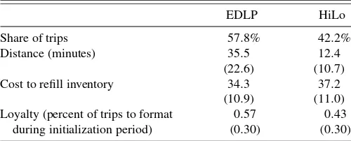
Consistent with Bell, Ho, and Tang (1998), we identified re-tailers as being either EDLP or HiLo based on their advertised pricing strategy. This resulted in three EDLP retailers and four HiLo retailers. The EDLP (HiLo) retailers had 58% (42%) of the shopping trips. To determine distance between a panelist and a store, we use the travel time (in minutes) from a pan-elist’s zip+4 to the store’s location (for privacy reasons, the panelist’s actual street address is not included in the data).
Table 1. Descriptive statistics for the households
Mean SD
Number of households 161
Average monthly spending $233.9 85.4
Minimum monthly spending $102.2 61.9
Number of shopping trips 184.2 83.4
Av. days between trips 4.6 1.8
Av. spending per trip 36.5 15.8
Elderly 13.7% 34.5%
Household size 2.9 1.3
Income (,000) $56.2 $25.0
College 41.0% 49.3%
Married 82.0% 38.5%
Table 2. Price format statistics
EDLP HiLo
Share of trips 57.8% 42.2%
Distance (minutes) 35.5 12.4
(22.6) (10.7)
Cost to refill inventory 34.3 37.2
(10.9) (11.0)
Loyalty (percent of trips to format 0.57 0.43
during initialization period) (0.30) (0.30)
We have detailed price information for 289 categories and, of these categories, we selected 150 categories based upon the following criteria. First, three common UPCs had to be carried by each retailer so that category price indices could be com-puted. Second, at least 5% of the selected households had to make at least three purchases in the category to ensure that the category is substantial. Third, the category had to account for at least 0.9% of total basket spending for the selected households. These categories together comprise more than 88% of the mar-ket basmar-ket on average (excluding fresh meat, fruit, and vegeta-bles). So, we use these categories to estimate the cost at each format. While not reported here, details of the categories are available from the authors. Table2shows specific statistics for the price formats with the standard deviations in parentheses. Note that the description of cost to refill inventory is provided in the next section.
6.2 Data Aggregation
Because our focus is on consumers selecting a type of store format (EDLP versus HiLo) rather than selecting a specific store, we need to aggregate our store-level data to the format level. This aggregation is done based on the proportion of a household’s visits to each store during the initialization period defined previously. Specifically, letFEbe the set of stores with an EDLP price format, FH be the set of stores using a HiLo format, andDhs be the distance from household h’s home to stores. The distance from householdhto formatf can be de-fined asDh,f=s∈Ff wh,f,sDh,s, wherewh,f,sis the proportion
of visits to storesmade by householdhin the initialization pe-riod andFf is eitherFEorFH.
Because the cost to replenish the inventory (also called “cost”) for a household, Sth,f on a shopping occasion is not observed prior to the visit, we need to create a measure of cost for each trip. The general goal is to create a time-varying, household-specific index for each store. This index is then ag-gregated to the format level similar to distance above. Clearly, the cost at storesin periodtby householdh, denotedSth,s, is the sum of the cost to the household in each category,c=1, . . . ,C the household will purchase in periodt (Bell, Ho, and Tang 1998). Therefore, cost can be written as
E[Sth,s] =
C
c=1
E[pth,s,c]E[qth,c], (3) whereE[pth,s,c]is the expected price of categorycat storesin periodtfor householdhandE[qth,c]is the quantity householdh needs to purchase in categorycin periodtto replenish its inven-tory. For price, we construct “market average” price indices for
the EDLP and HiLo retailers based upon the retailers’ long-run share of visits, that is, visits over the entire estimation sample. The second component on the right-hand side of Equation (3) is the quantity that needs to be replenished,E[qth,c]. Because we do not observe household inventories, we need a mecha-nism to predict this quantity using data that we, as researchers, observe—quantities purchased on previous occasions. We use Tobit models (that account for household heterogeneity) to pre-dict each household’s expected purchase quantity. Using the arguments found in Nevo and Hendel (2002) and elsewhere, we define (E[qth,c]) to depend upon the previous quantity pur-chased, the amount of time since last purchase, and the interac-tion between these terms as
E[qth,c]/q¯h,c
=β0,h+β1,h(qth,c−1/q¯h,c)+β2,h(dth,c/d¯hc)
+β3h((qh,ct−1/q¯hc)−1)((dth,c/d¯hc)−1)+ξh,ct , (4) whereqth,c is the quantity purchased in categorycin periodt by householdh,q¯h,cis the average quantity of categoryc pur-chased by householdhconditional on purchase in the category, dh,ct is the number of days since the category has been pur-chased,d¯hcis the average number of days between purchases in category c by household h, and ξh,ct is an error term that has normal distribution and is independent between categories. In the interaction term we subtract one (which is the mean of bothqth,c−1/q¯hcanddh,ct /dhc)from the quantity and time terms to allow clear definition ofβ1h andβ2h: β1h is the household response to quantity when the time between purchases is at the mean value, andβ2hrepresents household response to time when the average quantity was purchased on the prior occasion. The interaction term allows the household’s consumption rate to be nonconstant. The household coefficients in Equation (4) are assumed to have a normal distribution with mean β and standard deviation, where is a diagonal matrix. The key parameters of interest are lag quantity (expected sign is nega-tive), days since last category purchase (expected sign is pos-itive), and the interaction effect between these variables (ex-pected sign is positive).
Although not reported here, we find that, at the 5% level, 3 categories (2%) had positive and significant coefficients for lag quantity and 71 categories (47%) had negative and signifi-cant coefficients for lag quantity. Ninety-five (63%) categories had positive and significant coefficients for time since last cat-egory purchase and 13 (9%) had negative and significant coef-ficients for time since last category purchase. Forty-six (31%) had positive and significant coefficients for the interaction be-tween these variables, and 0 (0%) had negative and significant coefficients for the interaction. These results provide support for the models where the coefficients with incorrect signs are, in the aggregate, approximately 5% (16 of 450), which would be expected by chance.
We use the Tobit model results to predict the expected quan-tity required by each household in each period. We then follow the aggregation scheme from above to obtain the cost of visit-ing a specific format. Given the complexity and computational intensity of this method, we leave it for future research to de-termine methods that allow computationally feasible simulta-neous estimation of quantity and store choice. However, even
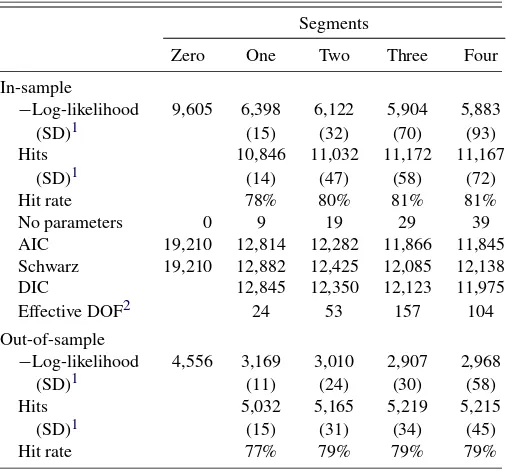
Table 3. Estimation results for parametric models
Segments
Zero One Two Three Four
In-sample
−Log-likelihood 9,605 6,398 6,122 5,904 5,883
(SD)1 (15) (32) (70) (93)
Hits 10,846 11,032 11,172 11,167
(SD)1 (14) (47) (58) (72)
Hit rate 78% 80% 81% 81%
No parameters 0 9 19 29 39
AIC 19,210 12,814 12,282 11,866 11,845
Schwarz 19,210 12,882 12,425 12,085 12,138
DIC 12,845 12,350 12,123 11,975
Effective DOF2 24 53 157 104
Out-of-sample
−Log-likelihood 4,556 3,169 3,010 2,907 2,968
(SD)1 (11) (24) (30) (58)
Hits 5,032 5,165 5,219 5,215
(SD)1 (15) (31) (34) (45)
Hit rate 77% 79% 79% 79%
1Standard deviations calculated using 25 bootstrap simulations.
2Effective Degrees of Freedom is defined as the difference between the mean of the bootstrap simulation liklihoods and the estimation sample likelihood; see Spiegelhalter et al. (2002).
in a parametric case, the problem of simultaneously estimat-ing 150 category equations and one format choice equation is formidable. (Note that we account for the estimation error in the standard errors by estimating Tobit models for each boot-strap simulation.)
6.3 Results
We also estimated a parametric model for model comparison. For this model, the function h(·)is defined as a simple linear specification:h(−Shft,−Dhf, ωs)=γ1sShft+γ2sDhf.
6.3.1 Model Selection. Table 3 provides the maximized likelihood values and information criteria for the estimation and holdout samples for one to four discrete segments. We calculate hits by assigning households to segments using the posterior probability of segment membership (see Kamakura and Russell 1989) then calculating the correct number of predicted choices using only that segment’s parameters to which the household is assigned. We use 25 bootstrap simulations to calculate the standard deviations of the model fit statistics across all models in both the parametric and semiparametric estimation.
The Schwarz criterion and the out-of-sample performance (log-likelihood and hit rate) indicate that the three-segment model is the “best” parametric model. Interestingly, the de-viance information criterion (DIC) suggests that the four-segment model is superior. However, we use the more conser-vative Schwarz criterion to avoid over-parameterization of the model. In the DIC, the effective degrees of freedom are calcu-lated as the difference between the likelihood of the estimation and the mean likelihood of the bootstrap simulations.
Given a three-segment parametric solution, we then esti-mated one through three segment solutions of the semiparamet-ric model. The results of the estimation are provided in Table4,
Table 4. Semiparametric estimation results
Segments
One1 Two Three
In-sample
−Log-likelihood 6,185 5,816 5,676
(SD)2 (22) (64) (30)
Hits 10,956 11,112 11,281
(SD)2 (30) (77) (36)
Hit rate 79% 80% 81%
No parameters 6 14 22
DIC 12,489 11,896 11,518
Effective DOF3 59 132 83
Out-of-sample
−Log-likelihood 3,224 2,993 2,892
(SD)2 (56) (50) (20)
Hits 5,093 5,248 5,270
(SD)2 (24) (33) (26)
Hit rate 77% 80% 80%
1The one-segment model is over-identified as the extant literature (Matzkin1992and Briesch, Chintagunta, and Matzkin2002) show that only one extra point and no parameter restrictions are required for identification of this model. We include this model for com-pleteness.
2Standard deviations calculated using 25 bootstrap simulations.
3Effective Degrees of Freedom is defined as the difference between the mean of the bootstrap simulation liklihoods and the estimation sample likelihood; see Spiegelhalter et al. (2002).
with the DIC indicating that the three-segment model is supe-rior. It is interesting to note that the improvement in the likeli-hood for using the one-segment semiparametric model versus the one-segment parametric model is similar to the
improve-ment in the two-segimprove-ment parametric model versus the one seg-ment parametric model. Therefore, replacing a linear function with a monotone function has an impact on the likelihood that is similar to the impact of adding heterogeneity and this rela-tionship remains as more discrete segments are added. This re-sult is consistent with the findings in Briesch, Chintagunta, and Matzkin (2002).
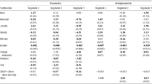
6.3.2 Model Results. Table5provides the maximum like-lihood estimator (MLE) parameter estimates from the three segment models for the parametric and semiparametric estima-tions, with the standard errors reported in parentheses. The seg-ments were matched based upon the size of the mass coeffi-cient, which roughly translates to the number of households in the segment. We note that this matching is arbitrary. Some of the key points are:
1. Demographic effects appear to be different across the parametric and semiparametric models. In the paramet-ric model, household size is significant and positive for all segments, while it is significant (and negative) for only one segment in the semiparametric model. College edu-cated head of household is significant for all of the semi-parametric segments, while it is significant for only one of the parametric segments.
2. Loyalty effects appear to be similar for two of three seg-ments between the parametric and semiparametric mod-els. However, for segment three of the parametric model, the coefficient is negative and significant, unlike the iner-tia effects in the semiparametric model.
3. Finally, all of the distance and cost coefficients for the parametric model have the expected negative coefficients,
Table 5. MLE parameter estimates for three-segment model
Parametric Semiparametric
Coefficients Segment 1 Segment 2 Segment 3 Segment 1 Segment 2 Segment 3
Mass 1.27 0.12 0.00 0.00 −0.26 −1.50
(0.24) (0.29) (0.18) (0.34)
Intercept −0.20 3.23 −0.74 1.45 −0.01 −2.93
(0.07) (0.48) (0.15) (0.12) (0.07) (1.52)
Loyalty 2.61 3.31 −0.95 3.21 3.12 1.90
(0.03) (0.15) (0.19) (0.07) (0.04) (0.31)
Elderly −0.32 0.84 −4.51 −2.18 1.28 3.13
(0.05) (0.19) (0.29) (0.09) (0.09) (1.17)
HH size 0.05 0.38 0.28 0.02 −0.14 0.58
(0.01) (0.12) (0.02) (0.02) (0.02) (0.31)
Income 0.002 0.008 0.063 −0.007 −0.003 0.029
(0.001) (0.003) (0.004) (0.002) (0.001) (0.011)
College 0.06 1.56 −4.01 0.07 0.10 −0.92
educated (0.03) (7.92) (0.26) (0.07) (0.05) (0.40)
Distance −0.20 −0.85 −3.82
(0.01) (0.06) (0.21)
Cost −0.95 −2.33 −0.51
(0.19) (0.82) (0.38)
EDLP∗Days −0.01 −0.07 −0.14 −0.013 −0.013 −0.013
since last trip (0.01) (0.02) (0.02)
Theta 1.000 2.09 0.53
(0.01) (0.02)
NOTE: 1. One segment’s mass point set to zero for identification. 2.EDLP∗Dayssince last trip set to−0.013 for identification in semiparametric model. 3. One semiparametric theta constrained to one. 4. Segments are matched based upon mass values. 5. Bold values are significant atp<0.05.
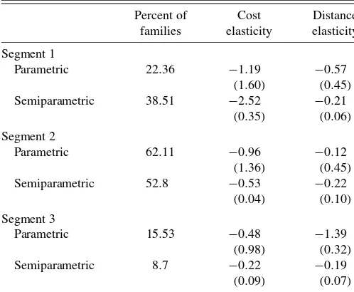
Table 6. Cost and distance elasticities by segment and model
Percent of Cost Distance
families elasticity elasticity
Segment 1
Parametric 22.36 −1.19 −0.57
(1.60) (0.45)
Semiparametric 38.51 −2.52 −0.21
(0.35) (0.06)
Segment 2
Parametric 62.11 −0.96 −0.12
(1.36) (0.45)
Semiparametric 52.8 −0.53 −0.22
(0.04) (0.10)
Segment 3
Parametric 15.53 −0.48 −1.39
(0.98) (0.32)
Semiparametric 8.7 −0.22 −0.19
(0.09) (0.07)
and these coefficients are significant at p<0.05 (one-tailed test).
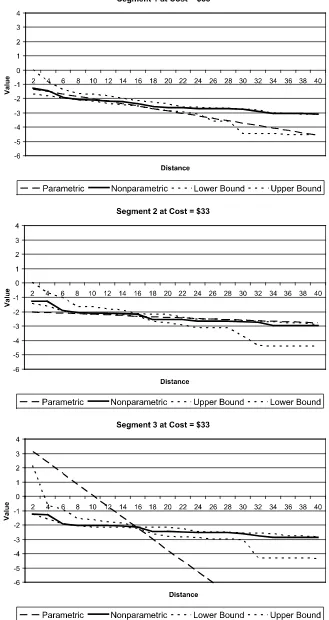
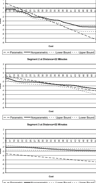
Now, we turn our attention to heterogeneity distribution of cost and distance sensitivities. Table6provides the elasticity es-timates for both parametric and semiparametric models as well as the percent of households assigned to each segment. First, the heterogeneity distribution is somewhat similar between the methods in an ordinal manner, that is, most of the families are in the moderate cost sensitivity segment (Segment 2), followed by the most cost sensitive segment (Segment 1) and the least cost sensitive segment (Segment 3). Second, the semiparamet-ric model indicates a larger range of cost sensitivity elastici-ties with a larger proportion of households being very cost sen-sitive. Third, the range of distance elasticities is larger in the parametric model. Indeed, the semiparametric model indicates less heterogeneity in distance sensitivities across households. These differences suggest that there are likely big differences in the response surfaces. Accordingly, the estimated response sur-faces for the variables of interest (cost and distance) are shown in Figures1 and2. Bootstrap simulations are used to get the semiparametric confidence intervals. The response surface for distance is plotted holding cost fixed at the mean value. Simi-larly, the response surface for cost is plotted holding distance fixed at the mean.
If we examine consumer response to distance (Figure1), we see that the semiparametric function is convex and decreasing. While not shown here, this convexity is pronounced at lower cost levels. This finding implies an interaction with the two vari-ables that would be required in a parametric representation of the model. We note that there are large differences in the para-metric versus semiparapara-metric functions, with the former having much larger slopes and different intercepts.
If we examine consumer response to cost (Figure2), we also find differences between the parametric and semiparametric re-sponse surfaces. While not shown here, in the semiparamet-ric case, we see an interaction effect with distance. At large distances, the response surface is almost flat. However, there are significant nonlinearities at shorter distances. The finding is
consistent with the “tipping point” argument made in Bell, Ho, and Tang (1998), although these results are much stronger.
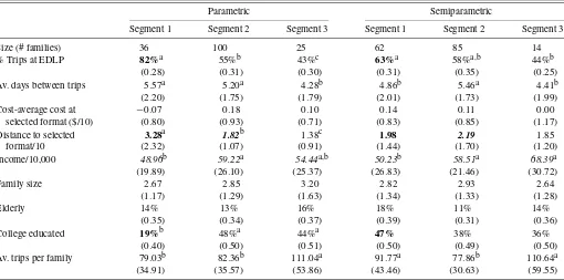
Finally, we examine the demographic profiles of the seg-ments in Table7. The significant differences (atp<0.05) be-tween the parametric and semiparametric models are shown in bold font in the table. There are three significant differences between the parametric and semiparametric results: percent of trips to EDLP retailer for Segment 1, average distance to se-lected formats in Segments 1 and 2 and college education of Segment 1. The average expected spending is similar for the segments but the number of trips (and hence total cost) is dif-ferent, as is the case in Bell, Ho, and Tang (1998).
7. CONCLUSIONS
We have presented a method to estimate discrete choice mod-els in the presence of unobserved heterogeneity. The method imposes weak assumptions on the systematic subutility func-tions and on the distribufunc-tions of the unobservable random vec-tors and the heterogeneity parameter. The estimavec-tors are com-putationally feasible and strongly consistent. We described how the estimator can be used to estimate a model of format choice. Key insights from the application include: (1) the parametric model provides different estimates of the heterogeneity distri-bution than the semiparametric model, (2) the semiparamet-ric model suggests interactions between cost and distance that change the shape of the response function, and (3) the benefit to adding semiparametric estimation is roughly equal in magni-tude to adding heterogeneity to parametric models. The benefit remains as the number of segments increases.
One drawback of the method is the computational time. The amount of time required to estimate the model is proportional to how good the starting point is. We used the one-segment semi-parametric solution as a starting point for the three-segment so-lution and it took approximately two weeks for the first simula-tion to complete on a 1 GHz personal computer (the bootstrap simulations took a much shorter amount of time as they used the three-segment solution as a starting point). As computing power becomes cheaper, this should be less of a problem.
Some variations on the model presented in the above sections are possible. For example, instead of lettingV(j,s,xj,rj, ω)=
v(j,s,xj, ω)−rj, where rj ∈ R+, one can let rj be an L -dimensional vector, and specify V(j,s,xj,rj, ω) =v(j,s,xj,
ω)−β·rj. Assuming that one coordinate ofβ equals one, it is possible to identifyβ and all the functions and distributions that were identified in the original model. Another variation is obtained by eliminating the unobservable random variablesεj. WhenV(j,s,xj,rj, ω)=v(j,s,xj, ω)−rj, the distribution ofω and the functionsv(j,·)are identified as well.
Future extensions of the model will deal with the case where the heterogeneity parameterωis multidimensional and the case where the vector of observable exogenous variables (s,z1, . . . ,zJ) is not necessarily independent of either ω or (ε1, . . . , εJ) (Matzkin2005).
APPENDIX: THEOREM PROOFS Proof of Theorem1
Letηj=(ε1−εj, . . . , εJ−εj) (j=1, . . . ,J). To recover the distribution of ηk for all k=1, . . . ,J it is enough to deter-mine the identification of F1∗ (see Thompson 1989). So, let
Figure 1. Segment distance response surface at mean cost.
Figure 2. Segment cost response surface at mean distance.