J A N U A RY 2 0 1 4
An Accuracy Assessment
of the
Global Employment
Trends’
Unemployment
Rate Forecasts
An Accuracy Assessment of the
Global
Employment Trends’
Unemployment
Rate Forecasts
Evangelia Bourmpoula and Christina Wieser*
January 2014
International Labour Office
________________
First published 2014
Publications of the International Labour Office enjoy copyright under Protocol 2 of the Universal Copyright Convention. Nevertheless, short excerpts from them may be reproduced without authorization, on condition that the source is indicated. For rights of reproduction or translation, application should be made to ILO Publications (Rights and Permissions), International Labour Office, CH - 1211 Geneva 22 (Switzerland) or by email:[email protected]. The International Labour Office welcomes such applications.
Libraries, institutions and other users registered with reproduction rights organisations may make copies in accordance with the licences issued to them for this purpose. Visit http:/ifrro.org to find the reproduction rights organisation in your country.
The designations employed in ILO publications, which are in conformity with United Nations practice, and the presentation of material therein do not imply the expression of any opinion whatsoever on the part of the International Labour Office concerning the legal status of any country, area or territory or of its authorities, or concerning the delimitation of its frontiers.
The responsibility for opinions expressed in signed articles, studies and other contributions rests solely with their authors, and publication does not constitute an endorsement by the International Labour Office of the opinions expressed in them. Reference to names of firms and commercial products and processes does not imply their endorsement by the International Labour Office, and any failure to mention a particular firm, commercial product or process is not a sign of disapproval.
Acknowledgements
Abstract
This study provides a quantitative assessment of the bias, accuracy, and efficiency of the Global Employment Trends (GET) global and regional unemployment rate forecasts made in three recent annual GET reports. After conducting a series of statistical tests, the results suggest that, on average across all countries with data availability, the GET unemployment rate forecasts are slightly biased; we over-predict one and two years ahead and under-predict three and four years ahead. However, this bias is not significant for one to three years ahead. Moreover, our tests for accuracy show that the shorter the prediction period, the more accurate our forecasts indicated by smaller forecast errors for shorter prediction periods and larger forecast errors for longer periods.
Keywords: forecasts, unemployment rate, bias, accuracy, efficiency
Abbreviations
AFE Average forecast error
EU European Union
GDP Gross Domestic Product
GET Global Employment Trends
ILO International Labour Organization IMF International Monetary Fund
MAE Mean absolute forecast error
MedAE Median absolute forecast error MedSE Median squared forecast error
MSE Mean squared forecast error
RMSE Root mean squared forecast error UB Bias proportion of MSE
UC Covariance proportion of MSE
Contents
Acknowledgements ... iii
Abstract ... iv
Abbreviations ... v
1. Introduction ... 1
2. Description of the dataset ... 3
3. Properties of good forecasts and measures used ... 4
3.1 Bias ... 4
3.2 Accuracy ... 5
3.3 Informational efficiency ... 6
4. Summary statistics of forecast errors ... 6
4.1 Global summary statistics ... 6
4.2 Regional summary statistics ... 11
5. Comparison of unemployment rates with GDP growth rate revisions ... 19
5.1 Testing for bias ... 20
5.2 Testing for accuracy ... 21
5.3 Testing for informational efficiency ... 22
6. GET forecasts vs. alternative forecasts ... 23
6.1 Testing for bias ... 23
6.2 Testing for accuracy ... 25
6.3 Testing for informational accuracy ... 25
7. Conclusions and further work ... 26
References ... 29
Annexes ... 31
Annex 1. Literature on forecast errors and measures used ... 31
Annex 2. Tables ... 32
Annex 3. Definitions of summary statistics ... 46
Annex 4. Reported rates ... 47
Annex 5. Country groupings used in the Global Employment Trends Model and Reports ... 48
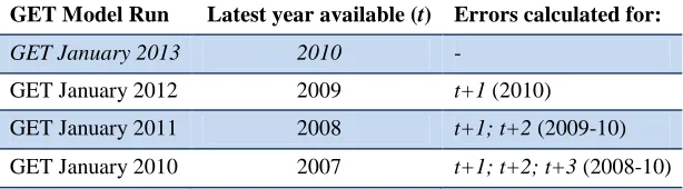
Tables Table 1. Example of error calculations for country X across the three GET Model runs ... 3
Table 2. Testing for bias, for global unemployment rate forecasts ... 8
Table 3. Summary of accuracy statistics for global unemployment rate forecasts ... 9
Table 4. Testing for efficiency, for global unemployment rate forecasts ... 10
Table 5. Testing for bias, for Developed Economies and EU unemployment rate forecasts ... 11
Table 6. Summary of accuracy statistics for unemployment rate forecasts in the Developed Economies and EU ... 11
Table 7. Testing for efficiency, for Developed Economies and EU unemployment rate forecasts ... 12
Table 8. Testing for bias, for Central and South-Eastern Europe (non-EU) and CIS unemployment rate forecasts ... 13
Table 9. Summary of accuracy statistics for unemployment rate forecasts in Central and South-Eastern Europe (non-EU) and CIS... 13
Table 10. Testing for efficiency, for Central and South-Eastern Europe (non-EU) and CIS unemployment rate forecasts ... 13
Table 12. Summary of accuracy statistics for unemployment rate forecasts in Asia ... 14
Table 13. Testing for efficiency, for Asia unemployment rate forecasts ... 15
Table 14. Testing for bias, for Latin America and the Caribbean unemployment rate forecasts ... 15
Table 15. Summary of accuracy statistics for unemployment rate forecasts in Latin America and the Caribbean ... 16
Table 16. Testing for efficiency, for Latin America and the Caribbean unemployment rate forecasts ... 16
Table 17. Testing for bias, for the Middle East and Africa unemployment rate forecasts... 17
Table 18. Summary of accuracy statistics for unemployment rate forecasts in the Middle East and Africa ... 17
Table 19. Testing for efficiency, for the Middle East and Africa unemployment rate forecasts ... 18
Table 20. Testing for bias, for global GDP growth revisions ... 21
Table 21. Summary of accuracy statistics for revisions of GDP growth rates ... 22
Table 22. Testing for efficiency, for global GDP growth revisions ... 22
Table 23. Testing for bias, baseline forecasts ... 24
Table 24. Comparison accuracy statistics GET forecasts and alternative forecasts ... 25
Table 25. Testing for efficiency, baseline forecasts ... 26
Annex Tables Table A1. Evaluation of forecast performance in selected literature ... 31
Table B1. Summary statistics of actual and forecasted unemployment rates ... 32
Table B2. Summary of accuracy statistics for the GET unemployment rate forecasts ... 33
Table B3. Testing for bias ... 35
Table B4. Testing for efficiency ... 36
Table B5. Summary statistics of latest and revised GDP growth rates ... 37
Table B6. Summary of accuracy statistics for the revisions of GDP growth rates ... 38
Table B7. Testing for bias, GDP revisions ... 40
Table B8. Testing for efficiency, GDP revisions ... 41
Table B9. Summary accuracy statistics for unemployment rate forecasts based on the baseline model ... 42
Table B10. Testing for bias, baseline forecasts ... 44
Table B11. Testing for efficiency, baseline forecasts ... 45
Table D1. Reported total unemployment rates by year and by run (units) ... 47
Figures Figure 1. Actual versus forecasted rates ... 7
Figure 2. Distribution of errors ... 8
Figure 3. Annual real GDP growth rate, selected economies ... 19
Figure 4. Actual vs. forecasted unemployment and unemployment rate, selected economies ... 20
Figure 5. Distribution of errors across alternative forecasts ... 24
1. Introduction
The annual Global Employment Trends (GET) is one of the International Labour Organization’s (ILO) flagship reports and analyses economic and social developments in labour markets, both globally and at the regional level. Taking into account the macroeconomic context, the report presents the employment and unemployment dynamics and provides estimates and forecasts of various labour market indicators such as unemployment, employment, status in employment, employment by sector, working poverty and labour productivity.
The GET model is one of the main data sources feeding the GET report. The GET model was built to provide consistent and comparable estimates and short-term forecasts of labour market indicators, both globally and at the regional level. Relying on an empirically estimated Okun’s law, the output of the model is a complete dataset of 178 countries with the time series starting in 1991. In more detail, unemployment rate forecasts are obtained using the historical (negative) relationship between the unemployment rate and GDP growth (see Box 1).
Any forecast needs to be assessed in terms of its bias, accuracy, and efficiency. A thorough and systematic assessment of the quality can help inform efforts to improve forecasts. However, due to the short period for which forecasts are available, the quality of the GET unemployment rate forecasts has not yet been evaluated in a systematic manner. This note aims to address this gap by providing a quantitative assessment of the bias, accuracy, and efficiency of the GET global and regional unemployment rate forecasts made in three recent annual GET reports that were released each year in January (ILO 2010b, 2011, 2012). The purpose is not to examine each individual model run but rather to evaluate the average performance of all forecasts over the last three years against the actual outcomes and alternative forecasts. This note therefore conducts a series of statistical tests to evaluate the quality of the ILO unemployment rate forecasts and to assess whether forecasts were unbiased, accurate, and informatively efficient.
Box 1. Note on global and regional projections
Unemployment rate projections are obtained using the historical relationship between unemployment rates and GDP growth during the worst crisis/downturn period for each country between 1991 and 2005 and during the corresponding recovery period.1 This was done through the inclusion of interaction terms of crisis and recovery dummy variables with GDP growth in fixed effects panel regressions.2 Specifically, the logistically transformed unemployment rate was regressed on a set of covariates, including the lagged unemployment rate, the GDP growth rate, the lagged GDP growth rate and a set of covariates consisting of the interaction of the crisis dummy, and of the interaction of the recovery dummy with each of the other variables.
Separate panel regressions were run across three different groupings of countries and are controlled for by using fixed effects in the regressions, based on:
1) geographic proximity and economic/institutional similarities; 2) income levels;
3) level of export dependence (measured as exports as a percentage of GDP).
The rationale behind these groupings is the following: countries within the same geographic area or with similar economic/institutional characteristics are likely to be similarly affected by the crisis, and have similar mechanisms to attenuate the crisis impact on their labour markets. Furthermore, because countries within geographic areas often have strong trade and financial linkages, the crisis is likely to spill over from one economy to its neighbour (e.g. Canada’s economy and labour market developments are intricately linked to developments in the United States). Countries of similar income levels are also likely to have more similar labour market institutions (e.g. social protection measures) and similar capacities to implement fiscal stimulus and other policies to counter the crisis impact. Finally, as the decline in exports was the primary crisis transmission channel from developed to developing economies, countries were grouped according to their level of exposure to this channel, as measured by their exports as a percentage of GDP. The impact of the crisis on labour markets through the export channel also depends on the type of exports (the affected sectors of the economy), the share of domestic value added in exports, and the relative importance of domestic consumption (for instance, countries such as India or Indonesia with a large domestic market were less vulnerable than countries such as Singapore and Thailand). These characteristics are controlled for by using fixed-effects in the regressions.
In addition to the panel regressions, country-level regressions were run for countries with sufficient data. The ordinary least-squares country-level regressions included the same variables as the panel regressions. The final projection was generated as a simple average of the estimates obtained from the three group panel regression and, for countries with sufficient data, the country-level regressions as well.
For more information on the methodology of producing world and regional estimates, see www.ilo.org/trends and ILO (2010a).
1
The crisis period comprises the span between the year in which a country experienced the largest drop in GDP growth, and the “turning point year”, when growth reached its lowest level following the crisis, before starting to climb back to its pre-crisis level. The recovery period comprises the years between the “turning point year” and the year when growth has returned to its pre-crisis level.
2
2. Description of the dataset
The GET model was built in 2003 and its first (current year) forecast was used in the GET 2004 report (Crespi, 2004; ILO, 2004). The GET model was initially developed to provide annual estimates of unemployment rates about once per year. However, in 2009, there was a need to evaluate more often the rapidly worsening conditions in the labour market due to the highly uncertain economic environment. Hence, the GET model was extended and has been run more frequently since (ILO, 2010a). The first forecasts from the model’s extension were utilized in the GET 2010 report (ILO, 2010b) and we therefore examine the most recent set of forecasts that were analysed in the three latest annual GET reports (ILO 2010b, 2011, 2012) in this post-mortem analysis. We treat the available (reported) rates in the most recent GET 2013 report (ILO, 2013) as our final/actual rates and use them to calculate the forecast errors.3
The latest available year for which a comparison of forecasted unemployment rates and actual values is possible, is 2012 and these results were displayed in the GET 2013 (see Annex 4). However, we also include forecasts prior to 2010 to increase our sample size if reported (actual) data were not included in the respective GET model run. Our calculations therefore start in 2007 and a maximum of four forecast periods are examined: one to four years ahead. We use 2007 as the cut-off year due to our interest in examining the forecasting performance of the model during the most recent years and due to the fact that 2007 is the latest year across all four runs with relatively high reporting rates. On average, there are 92 predictions for one year ahead, 86 for two years ahead, 82 for three years ahead and only 61 for 4 years ahead.
In the example in Table 1, the earliest year included in the analysis for the GET January 2010, is 2007, for the GET January 2011, the earliest year included is 2008 and so forth. As a result, a maximum of three errors can be calculated for the GET January 2010 model run (i.e. for 2007−09), two errors for the GET January 2011 model run (i.e. for 2008−09) and one error for the GET January 2012 model run (i.e. 2009).
Table 1. Example of error calculations for country X across the three GET Model runs
GET Model Run Latest year available (t) Errors calculated for:
GET January 2013 2010 -
GET January 2012 2009 t+1 (2010)
GET January 2011 2008 t+1; t+2 (2009-10)
GET January 2010 2007 t+1; t+2; t+3 (2008-10)
To avoid including data revisions in the calculation of errors, we exclude countries for which historical data series have been revised (e.g. change in the repository or source used, past-revised series, etc.). As a result, 15 countries were excluded from at least one of the three model runs under examination.
3
3. Properties of
good
forecasts and measures used
The predictive power of any model depends on the quality of the data used, the forecast horizon, as well as the statistical measures for its evaluation. There are three fundamental properties of a good forecast: bias, accuracy, and informational efficiency (Makridakis et al., 1998; Timmermann, 2006, 2007; Vogel, 2007; Leal et al., 2008).4 This section is divided into these three forecast properties and GET forecasts are evaluated according to these properties.
In general, a best forecast has a zero average forecast error and predicts the direction correctly. It also uses all available and relevant information at the time of the forecast so that the forecast errors are random and uncorrelated over time (i.e. serially uncorrelated). An optimal forecast should also have declining variance of forecast error as the forecast horizon shortens. There is a large body of literature on the evaluation of forecast performance and used statistics.
Table A1Table A1 in Annex 1 summarizes selected literature and the measures used to evaluate forecast performance.
For this post-mortem analysis we chose a combination of measures most commonly used in the literature to evaluate the performance of the GET forecasts. Measures were chosen according to their compatibility with data constraints, simplicity of interpretation and inclusion of a wide enough range of measures to analyse bias, accuracy, and informational efficiency of the GET forecasts. Each of the measures is briefly summarized below.
3.1 Bias
A forecast is said to be unbiased if the forecast does not show a tendency to go in either direction (over- and under-prediction). The average forecast error (AFE) gives an indication about the projection bias with values close to zero indicating unbiased predictions. Average forecast errors are said to be over-predicted if the predicted rate is larger than the actual rate (AFE has a negative sign) and under-predicted if the predicted rate is smaller than the actual rate (AFE has a positive sign).
Furthermore, kurtosis and skewness of the error distribution give information about the bias as both indicators measure the shape of the distribution. Kurtosis measures how steep the peak of the distribution is and skewness measures how much the distribution leans towards the right or left hand-side of the mean.
The most common indicator for kurtosis is the excess kurtosis which compares the shape of the distribution with the shape of a normal distribution.5 Therefore, in the case of over- or under-prediction, we expect non-zero excess kurtosis, meaning that the variance of the distribution is mostly influenced by infrequent extreme deviations. Negative excess kurtosis indicates flatter/wider peaks, compared to positive excess kurtosis indicating steeper peaks.
4 The common assumptions is a symmetric quadratic loss function, but for an overview of properties of good
forecasts under asymmetric loss function and nonlinear data generating processes, see Patton and Timmermann (2007).
Regarding skewness, a positive skew occurs when the right-hand side tail is longer than the left-hand side tail. In this case, positive errors are more common and hence under-prediction takes place (i.e. the predicted rate is smaller than the actual rate). Similarly, a negative skew occurs when the left-hand side tail is longer than on the right-hand side and over-prediction is more common. Therefore, we expect a right-skewed distribution to be associated with under-prediction and a left-skewed distribution with over-prediction. These measures though are only briefly discussed at a global level.
Despite the fact that we are restricted to a short period of forecast errors (maximum of four errors can be calculated, see section 2), the following simple Ordinary Least Squares (OLS) regression is run as a pooled panel to test for forecast bias:
= + (1)
where = − is the forecast error (averaged across the three model runs), stands for available (actual) observation, stands for forecasted observation, stands for the year ahead from the latest available observation (1,2,3,4), stands for country and is a stochastic term. For an unbiased forecast, the constant of regression 1 should be zero.
3.2 Accuracy
Forecast measures are said to be accurate if the size of the forecast error is small and the forecast has the capability to predict the right direction of the actual outcome (Leal et al., 2008). Various tools are available to measure this predictability of the realization of forecasts of which the ones used in this post-mortem analysis will be discussed.
The mean absolute forecast error (MAE) measures the absolute magnitude of the error and the closer to zero the MAE, the more accurate the forecast. In addition, the root mean squared forecast
error (RMSE), just as the MAE, assumes a symmetric loss function for projection errors (i.e. equal
weights to over- and under-predictions) but larger errors are penalized to a greater extent due to the squared computation. It measures the deviation of the forecast from the actual value and it is compatible with a quadratic loss function.
Due to extreme values, only considering mean forecast errors can be misleading. As a result, we also calculate the median absolute forecast error (MedAE) and median squared forecast error (MedSE) as alternative measures for accuracy. Values close to zero indicate accurate predictions and in cases in which the mean and the median are equal, the distribution of errors is closer to normal.
Furthermore, we also consider the mean squared forecast error (MSE) and decompose it into a bias proportion, a variance proportion, and a covariance proportion (see e.g. Koutsogeorgopoulou, 2000). The bias proportion (UB) measures the deviation of the mean prediction from the mean actual value and gives an indication for systematic forecast error. The variance proportion (UV) measures the error in forecasting the systematic component of variation of the actual values, and the covariance
proportion (UC) measures the error in forecasting the unsystematic component of the variance of the
actual values. For a forecast to be accurate, the UC of the MSE is closer to unity and the UB and UV are close to zero (Koutsogeorgopoulou, 2000).
variation in the actual data. Values close to zero indicate that the projections are “uninformative”, meaning that the projection errors have similar variation to the actual outcomes (Vogel, 2007).
3.3 Informational efficiency
Informational efficiency contains two dimensions, 1) whether information is available and 2) to what extent this information is used. An optimal forecast would contain all available information efficiently and would therefore not produce forecast errors (Timmermann, 2007). The informational efficiency can be tested with the simple OLS regression:
= + + (2)
where stands for available (actual) observation, stands for forecasted observation, stands for the year ahead from the latest available observation (1,2,3,4), stands for country and is a stochastic term. For an efficient forecast, the constant of regression 2 should equal zero and the regression coefficient should equal unity (Koutsogeorgopoulou, 2000).
4. Summary statistics of forecast errors
4.1 Global summary statistics
A good forecast should be unbiased, show small errors and should incorporate all relevant information so that forecast errors that do appear are random (Vogel, 2007). Summary statistics of statistical error analysis and regression analysis display that these conditions are partially met with significant variations concerning different forecast horizons.
4.1.1 Testing for bias
The (unweighted) averages of the actual unemployment rates for those countries included in this post-mortem analysis were 9.2, 9.1, 9.0 and 8.7 per cent for one to four years ahead, while the (unweighted) averages of forecasted rates were 9.3, 9.2, 8.7 and 7.7 per cent, respectively (see Annex 2, Table B1). Figure 1 plots the actual vs. the forecasted unemployment rates.6 If a country is found precisely on the diagonal line, the forecasted rate is equal to the actual rate. If a country is found above (below) the line, the forecasted rate is larger (smaller) than the actual rate. For one and two years ahead, many observations (i.e. countries) are close to the 450 line with the majority of observations being above the line (i.e. over-predictions). Forecasts for three and four years are more concentrated under the line (i.e. under-predictions).
Using the AFE, results show that our GET forecasts were slightly biased; we over-predicted7 one and two years ahead by 0.1 percentage points on average at the global level and under-predicted8 over
6 Each country in the figure can comprise several observations. For example, for t+1, country X has several
observations, one comparing one year ahead forecast from the GET 2009 to the actual value, another one comparing one year ahead forecast from the GET 2010 to the actual value and so forth.
7
longer time horizons by 0.2 and almost 1 percentage points for three and four years ahead (see Annex 2, Table B1).
Figure 1. Actual versus forecasted rates
Note: The line in the figures indicates the 450 line. t + j refer to the jth year ahead forecast (j = 1,…,4).
Source: ILO calculations based on the Global Employment Trends (GET) January 2010; January 2011; January 2012; January 2013.
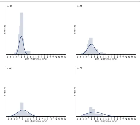
Similar results can be observed in Figure 2 which displays the distribution of errors for each forecast period. In all cases, the respective distribution is significantly different than the normal distribution. For one, three and four years ahead, the kurtosis and skewness are above 7 and 1, respectively, and for two years ahead the kurtosis is about 5 and the skewness about 0.7. However, by just looking at the figures, two, three and four years ahead show signs of right-hand skewness (i.e. under-prediction).
8
Figure 2. Distribution of errors
Source: ILO calculations based on the GET January 2010; January 2011; January 2012; January 2013.
Moreover, the results from equation 1 indicate that there was no significant bias for forecasts of one to three years ahead, but forecasts for four years ahead showed a positive bias indicating under-prediction (see Table 2 and Annex 2,Table B3).
Table 2. Testing for bias, for global unemployment rate forecasts
Year(s) ahead
1 2 3 4
World
α -0.0898 -0.0542 0.2473 0.9934***
(0.0749) (0.1372) (0.2182) (0.3683)
F (α=0) 1.4370 0.1561 1.2836 7.2771***
N 92 86 82 61
Note: Robust standard errors in parenthesis; *** p<0.01, ** p<0.05, * p<0.1 n = 92
In
c
id
e
n
c
e
0 1 2 3
-5 -4 -3 -2 -1 4 5 6 7 8 9 10 11 12 13 14 15 Error, t+1 (percentage points)
n = 86
In
c
id
e
n
c
e
-4 -2 0
-5 -3 -1 1 22 3 4 5 6 7 8 9 10 11 1213 14 15 Error, t+2 (percentage points)
n = 82
In
c
id
e
n
c
e
-5 -4 -3 -2 -1 0 1 2 3 4 5 6 7 88 9 10 11 123 13 14 15 Error, t+3 (percentage points)
n = 61
In
c
id
e
n
c
e
4.1.2 Testing for accuracy
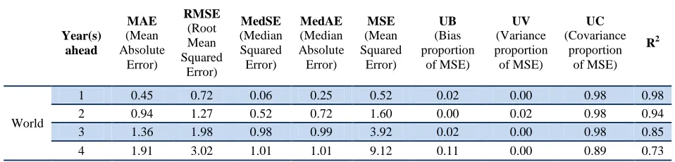
Applying the MAE to check for accuracy (the size of the absolute forecast error), we find that GET forecasts were more accurate the shorter the time horizon. In absolute terms, our one, two, three, and four years ahead forecasts were off by 0.5, 0.9, 1.4 and almost 2.4 percentage points respectively (see Table 3 and Annex 2, Table B2 for more details). The MedAE was smaller than the mean absolute error indicating that there were some extreme values that are punished to a greater extent in the mean absolute forecast error. Values close to zero indicate accurate predictions; the MedAE shows that 50 per cent of the range of MAE for one and two years ahead was below 0.2 and 0.7 percentage points, respectively. Similarly, for three and four years ahead, 50 per cent of the absolute forecast errors were below 1 percentage point.
Table 3. Summary of accuracy statistics for global unemployment rate forecasts
Year(s)
Source: ILO calculations based on the GET January 2010; January 2011; January 2012; January 2013.
According to the MAE and the MedAE, our forecasts for one and two years ahead were relatively accurate on average in comparison to longer term forecasts. The decomposition of the MSE into the bias and the variance proportion (UB and UV), which give an indication for systematic forecast errors and are close to zero for accurate forecasts, indicates that our forecasts one, two and three years ahead are indeed close to zero and therefore accurate (ranging from 0 to 2 per cent). However, for four years ahead, the bias proportion increases to 11 per cent. The co-variance proportion of the MSE (UC) also points to the accuracy of our forecasts one to three years ahead with a value close to unity of 98 per cent for one to three years ahead but only 89 per cent for the four years ahead forecasts.
Furthermore, based on the R2 of forecasts which indicates accuracy with values close to unity, 98, 94, 85 and only 73 per cent of the variation of the actual outcomes is captured by the forecasts for one, two, three, and four years ahead, respectively. Overall, the shorter the prediction period, the more accurate our forecasts; this result is also confirmed by the RMSE which increases largely with the time horizon of the forecasts.
In every GET report, the global and regional forecasts are accompanied with a confidence interval to acknowledge uncertainty around the baseline forecast, particularly during the economic crisis. Therefore, we also compare our errors with these confidence intervals (i.e. at the country level). We found that at the global level, one year ahead forecasts, 87 per cent of the errors were within the confidence interval (80 out of 92); for two years ahead forecast 84 per cent fall into the confidence interval (72 out of 86); for three years ahead 65 per cent also were not larger than the confidence interval (53 out of 82); and for four years ahead only 52 per cent of the errors lied within the confidence interval (32 out of 61).
unemployment rates away from their “average” predicted level. The largest forecast errors for four years ahead are mainly due to the crisis in Europe (for example, Cyprus, Greece, Spain) and the situation in countries on the periphery (for example Bulgaria, Croatia, Estonia) (see Figure 1). Since the GET model relies on an augmented concept of Okun's law, those highest forecast errors for the specific crisis period (especially for the four years ahead forecasts for 2007 for 2011) do not put the model into question.
4.1.3 Testing for informational efficiency
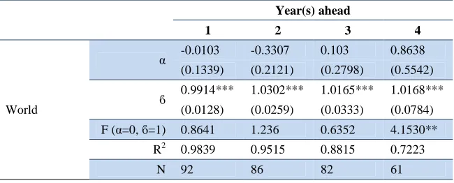
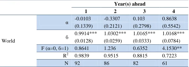
On average, our forecasts were informatively efficient, based on the results from equation 2 above (see Table 4 and Annex 2, Table B4). The results indicate that for one to three years ahead, the forecasts have informational value. The estimate for ϐ is significantly positive and very close to unity while the
estimate for the constant is not significant but close to zero.9 For forecasts of one to three years ahead, we do not reject the null joint hypothesis of informative forecasts (i.e. unity coefficient, zero constant and white-noise residuals). In the case of forecasts for four years ahead, the null hypothesis is rejected. However, for all four cases, the estimate for is not negative which would indicate misleading forecasts.
Table 4. Testing for efficiency, for global unemployment rate forecasts
Year(s) ahead
1 2 3 4
World
α -0.0103 -0.3307 0.103 0.8638
(0.1339) (0.2121) (0.2798) (0.5542)
ϐ 0.9914*** 1.0302*** 1.0165*** 1.0168***
(0.0128) (0.0259) (0.0333) (0.0784)
F (α=0, ϐ=1) 0.8641 1.236 0.6352 4.1530**
R2 0.9839 0.9515 0.8815 0.7223
N 92 86 82 61
Note: Robust standard errors in parenthesis; *** p<0.01, ** p<0.05, * p<0.1; R2 refers to the regression results.
4.1.4 Summary of world average
On average across all countries, we have some forecast bias; we slightly over-predict one and two years ahead and under-predict three and four years ahead. However, our regression analyses show that this bias is not significant for one to three years ahead. Overall, the shorter the prediction period, the more accurate our forecasts and our tests show that one to three years ahead were accurate but four years ahead were not. Nevertheless, in most cases the errors fall into the confidence intervals that accompanied the GET forecasts. Furthermore, our results also indicate that we have informational efficiency for one to three years ahead.
4.2 Regional summary statistics
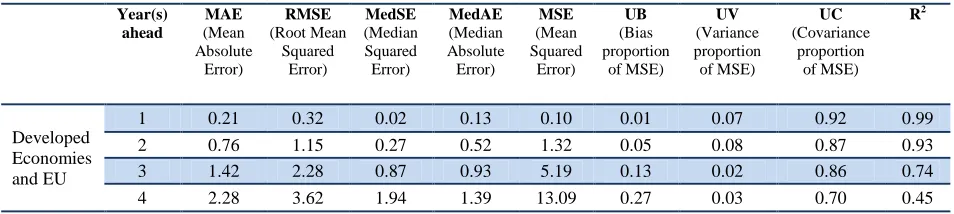
4.2.1 Developed Economies and European Union (EU)
Testing for bias
For the Developed Economies and European Union (EU) region where response rates are highest among all regions (see Annex 4, Figure D1), the (unweighted) average of actual unemployment rates were 8.7, 9.1, 9.1 and 9.4 per cent for one to four years ahead, respectively (see Annex 2, Table B1). The (unweighted) averages of the forecasted rates were 8.7, 8.8, 8.3 and 7.5 per cent for one to four years ahead, respectively.
On average, according to the AFE, we over-predict one year ahead by 0.04 points and under-predict two to four years ahead by 0.3, 0.8 and almost 2 percentage points respectively (see Annex 2, Table B1). Furthermore, the results from equation 1 indicate that there was no significant bias for forecasts of one to two years ahead, but the forecasts for three and four years ahead had a positive bias, implying under-prediction (see Table 5 and Annex2, Table B3).
Table 5. Testing for bias, for Developed Economies and EU unemployment rate forecasts
Year(s) ahead
Note: Robust standard errors in parenthesis; *** p<0.01, ** p<0.05, * p<0.1
Testing for accuracy
The median of the forecast errors’ distribution was below the mean pointing towards outliers with large forecast errors. In addition, for this region the forecasts for one and two years ahead were relatively accurate according to our error statistics but the forecasts for three and four years ahead were less precise. The bias proportion of the MSE (UB), which measures the deviation of the mean prediction form the mean actual value, was relatively small (and therefore accurate) for one and two years ahead, but it increased to about 13 and 27 per cent for the three and four years ahead (see Table 6 and Annex 2, Table B2). However, the variance proportion (UV), which measures the error in forecasting the systematic component of the variation of the actual values points to an accurate forecast as the levels stayed around zero for one to four years ahead.
Table 6. Summary of accuracy statistics for unemployment rate forecasts in the Developed
Based on the R2 of forecasts, the proportion of the variation of the actual values that was captured by the predictions was 99 and 93 per cent for one and two years ahead, but it dropped to 74 and 45 per cent for three and four years ahead, making our forecasts inaccurate for longer time horizons.
As already mentioned in section 4.1.2, the finding that three and four years ahead forecasts are not accurate is not surprising when taking the effects of the crisis into consideration, which had particularly severe consequences on unemployment in this region. The largest forecast errors for three and four years ahead are mainly due to the crisis in Europe. For example, in the GET 2010, the four years ahead forecast for Cyprus, Greece, Portugal and Spain was about 5, 9, 9 and 18 per cent, respectively, versus the realizations which were about 12, 24, 16 and 25 per cent, respectively.10
Testing for informational efficiency
Regression results to test for informational efficiency indicate that for one to two years ahead, the forecasts were informative. The estimate for ϐ was positive and significant and very close to unity
while we did not reject the null joint hypothesis of informative forecasts (see Table 7 and Annex 2, Table B4). However, the joint null hypothesis for three and four years ahead was rejected, confirming the previous results that the forecasts’ performance after two years ahead begins to deteriorate.
Table 7. Testing for efficiency, for Developed Economies and EU unemployment rate forecasts
Year(s) ahead
1 2 3 4
Developed Economies and EU
α 0.1558 -0.5141 0.1893 0.4828
(0.1294) (0.3862) (0.7389) (1.1423)
ϐ 0.9781*** 1.0880*** 1.0773*** 1.1878***
(0.0179) (0.0535) (0.1109) (0.1772)
F (α=0, ϐ=1) 0.7553 1.4916 3.1385* 6.8691***
R2 0.9937 0.9364 0.7756 0.6161
N 36 36 36 35
Note: Robust standard errors in parenthesis; *** p<0.01, ** p<0.05, * p<0.1; R2 refers to the regression results.
4.2.2 Central and South-Eastern Europe (non-EU) and Commonwealth of Independent States (CIS)
Testing for bias
For the sample of countries examined in the Central and South-Eastern Europe (non-EU) and CIS region, we under-predict unemployment rates by 0.04, 0.16, 0.01 and 0.3 percentage points for one, two, three, and four years ahead, respectively (see Annex 2, Table B1). Testing whether this bias is significant, we do not reject the null hypothesis (insignificance based on the results from equation 1) (see Table 8 and Annex 2, Table B3).
10 Similarly, the four years ahead GDP growth rate forecast in IMF/WEO October 2009 for the same countries
Table 8. Testing for bias, for Central and South-Eastern Europe (non-EU) and CIS
Note: Robust standard errors in parenthesis; *** p<0.01, ** p<0.05, * p<0.1
Testing for accuracy
The median of the forecast errors’ distribution was below the mean for all years ahead except for three years ahead. Our forecasts for this sample were relatively accurate for one and two years ahead which can be seen by the MedSE and MedAE as well as the proportion of the variation of the actual values that was captured by the forecasts; the R2 was 99 and 98 per cent, respectively. However, our accuracy for three and particularly for four years ahead dropped sharply, with an R2 down to 49 per cent for the four years ahead forecast (see Table 9). These results have to be taken with care because the sample size within this region was small, particularly for four years ahead (only six countries were included in the analysis).
Table 9. Summary of accuracy statistics for unemployment rate forecasts in Central and South-Eastern Europe (non-EU) and CIS
Year(s)
Source: ILO calculations based on the GET January 2010; January 2011; January 2012; January 2013.
Testing for informational efficiency
Based on the results from equation 2, the estimate for ϐ was positive, significant and very close to
4.2.3 Asia
Due to a relatively small sample of countries within each of the three sub-regions in Asia (East Asia, South-East Asia and the Pacific, and South Asia) we report the summary statistics within one section.
Testing for bias
For the sample of countries in Asia for which forecast errors were calculated, we infer that the volatility in both actual and forecasted unemployment rates was small. Our forecast for one year ahead was on average higher than the actual rate by 0.1, 0.2 and 0.3 percentage points in East Asia, South-East Asia and the Pacific; and South Asia, respectively (see AFE in Annex 2, Table B1).
However, the results from equation 1 also indicate that for Asia as a whole there was a negative bias (i.e. over-prediction) in the one to three years ahead forecasts (see Table 11 and Annex 2, Table B3).
Table 11. Testing for bias, for Asia unemployment rate forecasts
Year(s) ahead
Note: Robust standard errors in parenthesis; *** p<0.01, ** p<0.05, * p<0.1
Testing for accuracy
Due to the small number of forecast errors calculated, the conclusions drawn from the accuracy statistics were not robust. It appears that the forecast error did not decline the longer the prediction period was. For example, the RMSE for two years ahead for East and South Asia was larger than the RMSE for three and four years ahead, while for South-East Asia the RMSE was larger in the case of three years ahead than in the case of four years ahead (see Table 12).
Table 12. Summary of accuracy statistics for unemployment rate forecasts in Asia
Year(s)
Testing for informational efficiency
The regression results for Asia as a whole indicated efficient forecasts as the estimate for ϐ was
significantly positive and close to unity (see Table 13 and Annex 2, Table B4). However, we rejected the null joint hypothesis of informative forecasts.
Table 13. Testing for efficiency, for Asia unemployment rate forecasts
Year(s) ahead
1 2 3 4
Asia
α 0.0423 0.0048 0.1080 -0.1385
(0.1447) (0.3499) (0.3620) (0.4669)
ϐ 0.9517*** 08716*** 0.8746*** 0.9570***
(0.0275) (0.0726) (0.0769) (0.0819)
F (α=0, ϐ=1) 4.9828** 8.2241** 5.4244** 5.0726*
R2 0.9862 0.9423 0.9456 0.9179
N 11 10 10 8
Note: Robust standard errors in parenthesis; *** p<0.01, ** p<0.05, * p<0.1; R2 refers to the regression results.
4.2.4 Latin America and the Caribbean
Testing for bias
For the sample of Latin America and the Caribbean, we over-predict (we forecast higher unemployment rates than the actual values) by 0.3, 0.4, 0.01 and 0.3 percentage points for one, two, three, and four years ahead, respectively (see AFE in Annex 2, Table B1.
Based on the results from equation 1 though, there is no sign of a systematic bias as the α is negative
but not significant, and we do not reject the hypothesis that it is not significantly different from zero (see Table 14 and Annex 2, Table B3).
Table 14. Testing for bias, for Latin America and the Caribbean unemployment rate forecasts
Year(s) ahead
1 2 3 4
Latin America and the Caribbean
α -0.3121 -0.4475 -0.0329 -0.7546
(0.2098) (0.3056) (0.4495) (0.8230)
F (α=0) 2.2132 2.1443 0.0054 0.8407
N 22 20 18 7
Note: Robust standard errors in parenthesis; *** p<0.01, ** p<0.05, * p<0.1
Testing for accuracy
one, two and four years ahead are better than the three years ahead forecasts, with values ranging from
Source: ILO calculations based on the GET January 2010; January 2011; January 2012; January 2013.
Testing for informational efficiency
Regression results to test for informational efficiency indicate that the forecasts were informative. The estimate for ϐ was positive, significant and very close to unity. Although we reject the null hypothesis
of informative forecasts for the one year ahead forecast, the two to four years ahead forecast show that the ϐ and the α are not significantly different from unity and zero, respectively (see Table 16 and
Note: Robust standard errors in parenthesis; *** p<0.01, ** p<0.05, * p<0.1; R2 refers to the regression results.
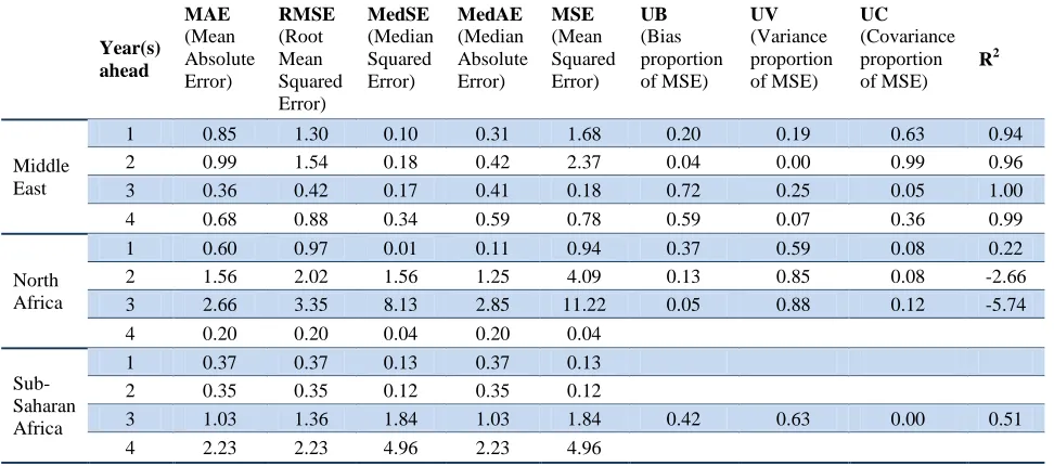
4.2.5 Middle East and Africa
The number of countries with forecast errors in the Middle East and Africa region was too small to infer robust results, particularly for accuracy (see Annex 2, Table B1and Table B2).
Testing for bias
Table 17. Testing for bias, for the Middle East and Africa unemployment rate forecasts
Note: Robust standard errors in parenthesis; *** p<0.01, ** p<0.05, * p<0.1
Testing for accuracy
For the Middle East, 50 per cent of the absolute errors for two years ahead was below 0.3 percentage points (see MedAE in Table 18 and Annex 2, Table B2). However, the bias proportion of MSE for the one year ahead forecast was far above zero (20 per cent). For the three countries for which forecast errors for three and four years ahead were calculated, we find that the longer the prediction period, the larger the RSME. For the sample in North Africa and Sub-Saharan Africa, again the shorter the forecast period, the more accurate the predictions were. However, in case of North Africa, there was an indication of misleading forecasts for two and three years ahead due to a negative R2 of forecasts.
Table 18. Summary of accuracy statistics for unemployment rate forecasts in the Middle East and Africa
Source: ILO calculations based on the GET January 2010; January 2011; January 2012; January 2013.
Testing for informational efficiency
The regression results for the Middle East and Africa as a whole indicate efficient forecasts as the estimate for ϐ was significantly positive and close to unity and the constant was close to zero and not
significant (see Table 19 and Annex 2, Table B4). In addition, we did not reject the null joint hypothesis of informative forecasts.
Table 19. Testing for efficiency, for the Middle East and Africa unemployment rate forecasts
Year(s) ahead
1 2 3 4
Middle East and Africa
α 0.9382 0.2423 0.4775 0.8218
(0.8581) (0.6604) (1.4749) (1.0258)
ϐ 0.9303*** 0.9676*** 0.9014*** 0.9293***
(0.0508) (0.0488) (0.1272) (0..0530)
F (α=0, ϐ=1) 1.0590 0.2222 0.4857 1.1361
R2 0.9429 0.9171 0.8476 0.9813
N 10 9 8 5
Note: Robust standard errors in parenthesis; *** p<0.01, ** p<0.05, * p<0.1; R2 refers to the regression results.
4.2.6 Summary regional analysis
Due to the short time horizon in our sample, regional analyses are not as meaningful in some regions as the global results. Nevertheless, there are some important lessons concerning forecast bias and accuracy from regional results.
In the Developed Economies and EU, the region with the largest sample size, there was no significant forecast bias for one to two years ahead, but a positive bias for three and four years ahead. Our forecasts for one and two years ahead capture 99 and 93 per cent of the variation of the actual values, while 92 and 87 per cent of the average squared forecast error is due to the unsystematic component of the variance of the actual values. Moreover, for one to two years ahead, the forecasts were informative. Similarly with the global results, the shorter the forecast period, the more accurate the predictions are.
For the Central and South-Eastern Europe (non-EU) and CIS region, we under-predicted unemployment rates, but our predictions were relatively accurate for one and two years ahead. Nevertheless, our regression results concluded that there is no systematic bias in all forecasts in this region, and also that the forecasts were informative. In addition, the unsystematic component of the variance of the actual values is mostly responsible for the forecast errors.
Due to the small number of forecast errors calculated in Asia, the conclusions drawn from the accuracy statistics were not robust. Furthermore, the regressions results indicate that there is a systematic bias in our forecasts but again the small sample size does not allow us to draw strong conclusions.
In Latin America and the Caribbean on the other hand, we forecasted higher unemployment rates than the actual values and in general, our forecasts were relatively accurate, particularly for one and two years ahead. The forecast bias is not significant for all forecasts, but for the one year ahead our forecasts are not informative.
5. Comparison of unemployment rates with GDP growth rate
revisions
As discussed above, the GET Model’s theoretical basis is Okun’s Law. Therefore, any revisions in the GDP growth rate forecasts also influence the forecasting performance of the unemployment rates. With the aim to relate the forecasting performance of unemployment rates and the revisions of GDP growth rates made by the International Monetary Fund in the World Economic Outlook Database (IMF WEO), we present a comparison of the two in this section. The comparison is directed at observing whether the direction and the size of the revisions of GDP growth rates are similar to the forecast errors of unemployment rates. To facilitate the comparison, we calculated similar indicators to the summary statistics of the unemployment rate, treating GDP forecast revisions as forecast errors.
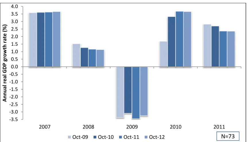
Figure 3 graphically presents the revisions made in the IMF WEO database for a sample of 73 countries based on the last three October updates. This sample is comprised of countries for which we have real unemployment rates for all years between 2007 and 2011 and hence, we also have forecasts errors calculated as an average across the three GET Model runs.
Figure 3. Annual real GDP growth rate, selected economies
Note: 73 countries are included in this figure (for which there has been at least one unemployment rate forecast between 2008 and 2011, based on one of the GET Model runs).
Source: ILO calculations based on International Monetary Fund, World Economic Outlook Database, October 2009; October 2010; October (released on September) 2011; October 2012.
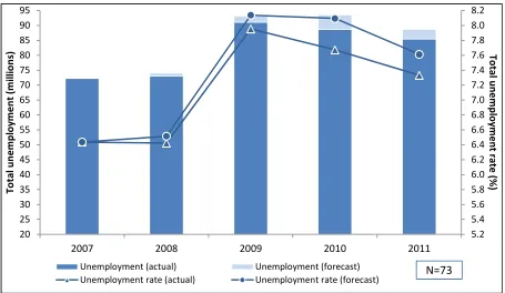
Actual and forecasted unemployment for the sample of countries utilized above are presented in Figure 4. In order to keep the number of countries the same for all years, a country with no forecast for a year was not excluded from the figure. Instead, the actual value is plotted for the year in which all GET Model runs had an actual rate (and thus no forecasts were made). This is only the case for some countries for 2008 for which, even in the earliest model run, data were available. In 2011, the GDP
2007 2008 2009 2010 2011
A
incurred a positive unemployment rate forecast error of 0.3 percentage points (actual unemployment of 7.3 per cent and forecasted unemployment rate of 7.6 per cent, see Figure 4). This 0.3 percentage point forecast error translates to an inaccurate estimation of the number of unemployed of more than 3 million.
Figure 4. Actual vs. forecasted unemployment and unemployment rate, selected economies
Note: 73 countries are included in this figure (for which there has been at least one unemployment rate forecast between 2008 and 2011, based on one of the GET Model runs). The unemployment numbers are benchmarked on the ILO Estimates and Projections of the Economically Active Population (EAPEP), 6th edition (Update July 2012).
Source: ILO calculations based on the GET January 2010; January 2011; January 2012; January 2013.
In this section, we will only report forecast errors at the global level, but more detail on each of the regions discussed in this paper can be found in Annex 2, Table B5, Table B6, Table B7 and Table B8.
5.1 Testing for bias
Overall, the (unweighted) average of actual GDP growth rates for the countries included in this post-mortem analysis were 1.5, 3, 2.9 and 2 per cent for one to four years ahead, while the (unweighted) average of the revised rate were 1.3, 2.6, 3.3 and 3.6 per cent, respectively (Annex 2, GDP growth rate, Table B5). The average forecast error (AFE) therefore indicates an over-prediction (the predicted GDP growth rate is higher than the revised rate) of 0.2 and 0.5 per cent for one and two years ahead, respectively, and an under-prediction of 0.4 and 1.6 per cent for three and four years ahead, respectively.
When comparing the results of GDP growth rates to the results of the world average of unemployment rates, the closely tied relationship of these two can be observed. An under-prediction of GDP growth rates for one and two years ahead results in an over-prediction of unemployment rates for the same time frame. Since forecasts for GDP growth rates were lower than the actual rates, forecasts for the
5.2
2007 2008 2009 2010 2011
T
GET unemployment rates were higher than the actual rates. It can also be observed, that the forecast bias of unemployment rates is much lower than the forecast bias of GDP growth rates for all years ahead.
It is worth mentioning here that it comes as no surprise that the output of the GET model (i.e. the unemployment forecast) is less noisy than the GDP forecasts that enter the model as a noisy input. This stems from the fact that the model also uses lags of unemployment rate (see ILO, 2010a). From an empirical observation, small revisions in the GDP growth series and small revisions/changes in unemployment rate data would roughly cause about 30 and 70 per cent of the changes in the final global numbers.
As expected, regression 1 run for GDP growth rates shows that the revisions are not done completely at random. The F-statistic rejects unbiasedness for all years’ revisions except the three years ahead (see Table 20 and Annex 2, Table B7). This result should be treated with care because a bias in revisions does not necessarily mean that the forecasts are biased. It might simply mean that the IMF receives the full components of the GDP or the final estimates (e.g. from the National Statistical Offices or Ministries) with a lag of one or two years and this might be the reason of a systematic upwards revision.
Table 20. Testing for bias, for global GDP growth revisions
Year(s) ahead
1 2 3 4
World
α 0.2304** 0.4688*** -0.3915 -1.6339***
(0.0920) (0.1642) (0.2457) (0.2877)
F (α=0) 6.2715** 8.1477*** 2.5388 32.2607***
N 87 81 78 58
Note: Robust standard errors in parenthesis; *** p<0.01, ** p<0.05, * p<0.1
5.2 Testing for accuracy
Table 21. Summary of accuracy statistics for revisions of GDP growth rates
Source: ILO calculations based on the GET January 2010; January 2011; January 2012; January 2013, and on IMF World Economic Outlook Database, October 2009; October 2010; October (released in September) 2011; October 2012.
Similarly to the results from equation 1, the decomposition of the MSE into the bias and the variance proportion (UB and UV) indicates that the GDP revisions are not unbiased (ranging from 1 to 11 per cent). The co-variance proportion of the MSE (UC) points to relatively low accuracy as compared to unemployment forecasts. Furthermore, based on the R2 of forecasts (i.e. revisions in the case of GDP) which indicates accuracy with values close to unity, 96, 82, 65 and only 59 per cent of the variation of the most recent estimates of GDP growth rates is captured by the past estimates for one, two, three, and four years ahead, respectively.
5.3 Testing for informational efficiency
Results from equation 2 confirm the biasedness of the revisions as seen previously, but the revisions are informative (see Table 22 and Annex 2, Table B8). The estimate for ϐ is close to unity and
significant. However, perhaps due to the size of the bias the F-statistic rejects the null joint hypothesis of informative revisions (i.e. unity coefficient, zero constant and white-noise residuals).
Table 22. Testing for efficiency, for global GDP growth revisions
Year(s) ahead
6. GET forecasts vs. alternative forecasts
As seen in section 3.1, one of the properties of an optimal forecast is that it provides additional information to alternatives (e.g. Vogel, 2007). The ILO is the only institution providing the public with global and regional forecasts of unemployment rates and we are therefore not able to compare our unemployment rates to other forecasts of unemployment rates. Thus, we therefore have to construct alternative forecast models to compare our results to; an obvious alternative to be examined is the naïve forecast model.
In general, a naïve forecast is one in which the actual value of the previous period is projected into the next period with the assumption that tomorrow will be like the last available observation. Due to its simplistic nature, it is often used as an alternative forecast model, such as in Ash et al. (1998). The results of the naïve forecast model show that the GET model outperforms the naïve model in every aspect (see Table 24). GET predictions are less biased, more accurate and contain a higher informational efficiency than the naïve forecasts.11
The alternative forecast used for comparison is similar to the naïve model but slightly more complex which for simplicity, we will call baseline forecast. This alternative forecast model to be chosen here, assumes a simple autoregressive model of second order with country dummies.12
= + + + + (3) where α is a constant, is the country-specific constant, and is a stochastic term. To estimate the coefficients we pooled all the countries together.
Figure 5 shows the distribution of the errors across the three alternative forecasts. Already this figure depicts that the GET forecasts errors are more concentrated around zero with steeper peaks for all forecast periods.
6.1 Testing for bias
Judging from the summary statistics of this baseline (simple autoregressive) model, on average, we would have under-predicted all years ahead by 0.3, 0.5, 0.6 and 1.3 percentage points and the actual unemployment rate would have been larger than the predicted rate(see AFE in Annex 2, Table B9). When comparing these baseline forecasts to the GET forecasts, we see that the average forecast error has a different bias for one and two years ahead but overall, is smaller for the GET forecasts. Moreover, the results from equation 1 clearly indicate that the baseline forecasts are significantly downwards biased for all years (see Table 23 and Annex 2, Table B10).
11 The results of the naïve forecast model are not shown in this report but are available upon request. Only the
distribution of the errors is shown in Figure 5 and some accuracy statistics in Table 24.
Figure 5. Distribution of errors across alternative forecasts
GET forecast
Baseline forecast (eq. 3)
Naive forecast
Source: ILO calculations based on the GET January 2010; January 2011; January 2012; January 2013.
Table 23. Testing for bias, baseline forecasts
Year(s) ahead
1 2 3 4
Baseline forecasts World
α 0.3428** 0.4906* 0.6261* 1.2837**
(0.1330) (0.2518) (0.3530) (0.4832)
F (α=0) 6.6454** 3.7942* 3.1460* 7.0585**
N 89 84 79 59
Note: Robust standard errors in parenthesis; *** p<0.01, ** p<0.05, * p<0.1
In
c
id
e
n
c
e
2
-10-9 -8 -7 -6-5-4 -3 -2 -1 0 1 3 4 5 6 7 8 910111213141516
Error, t+1 (percentage point)
In
c
id
e
n
c
e
-10 -9-8 -7-6 -5 -4 -3 -2 -1 0 1 2 33 4 5 66 77 88 9 10 11 1213 14 15 16
Error, t+2 (percentage point)
In
c
id
e
n
c
e
-10 -9 -8 -7 -6 -5 -4 -3 -2 -1 0 1 2 3 4 55 6 7 8 9 10 11 12 13 14 15 16
Error, t+3 (percentage point)
In
c
id
e
n
c
e
-10 -9 -8 -7 -6 -5 -4 -3 -2 -1 0 1 2 3 4 5 6 7 8 9 10 11 12 13 14 15 16
6.2 Testing for accuracy
When looking at our accuracy statistics, we observe that according to the mean absolute error, on average, the baseline forecasts would have been different than the actual value by 1, 1.5, 2.1 and 2.5 points for one up to four years ahead, respectively (see Table 24). These values point to a more inaccurate forecast using the baseline model than using our GET model. These results are backed up by other accuracy statistics, such as the median squared error and the median absolute error which are all further away from zero than our GET forecasts for all time periods.
Table 24. Comparison accuracy statistics GET forecasts and alternative forecasts
Year(s)
Source: ILO calculations based on the GET January 2010; January 2011; January 2012; January 2013.
Even though the deviation of the mean prediction from the mean actual value (measured by the bias proportion of the mean squared error) for the baseline forecasts points towards no systematic component of the forecast error, the GET forecasts still performed better. However, measuring the variance proportion as well as the covariance proportion, the baseline forecast would have performed slightly better than the GET forecast indicating a better prediction of the systematic and unsystematic component of variation of the actual values with the baseline forecasts. However, based on the R2 of forecasts, our GET forecasts perform better concerning the variation of the actual values which the predictions have correctly taken into account. The baseline forecasts show that only 93, 80, 61 and only 56 per cent of the variation of the actual outcomes would have been captured by these forecasts for one up to four years ahead, respectively. Therefore, at least for this sample of results, the GET unemployment rate forecasts have been superior to the alternative.
6.3 Testing for informational accuracy
Regarding the results from equation 2, although the estimate for ϐ is close to unity and significant, for
Table 25. Testing for efficiency, baseline forecasts
Year(s) ahead
1 2 3 4
Baseline forecasts World
α 0.1074 -0.0434 0.8166 1.9764***
(0.2839) (0.4912) (0.5291) (0.7122)
ϐ 1.0272*** 1.0607*** 0.9787*** 0.9079***
(0.0361) (0.0682) (0.0731) (0.1071)
F (α=0, ϐ=1) 3.4096** 1.9196 2.6579* 6.4875***
R2 0.9449 0.8392 0.7028 0.5390
N 89 84 79 59
Note: Robust standard errors in parenthesis; *** p<0.01, ** p<0.05, * p<0.1; R2 refers to the regression results.
Overall, it is shown that the GET forecasts produce less biased, more accurate and more informatively efficient results than our alternatives.
7. Conclusions and further work
The results in this post-mortem analysis of the GET unemployment rates suggest that, on average across all countries for which data are available, the GET unemployment rate forecasts are slightly biased; that is we over-predict one and two years ahead and under-predict three and four years ahead. However, this bias is not significant for one to three years ahead.
In general, our tests for accuracy show that the shorter the prediction period, the more accurate our forecasts indicated by smaller forecast errors for shorter prediction periods and larger forecast errors for longer periods. The one, two, and three years ahead forecasts were accurate; however, the four years ahead forecast was inaccurate. Furthermore, our results also indicate that we have informational efficiency for one to three years ahead.
Regional comparisons are difficult due to the small sample size resulting from the short time horizon in our sample. Nevertheless, there are some important lessons to be learned concerning forecast bias and accuracy from regional results. In the Developed Economies and the EU, the region with the largest sample size, there was no significant forecast bias for one to two years ahead, but a positive bias for three and four years ahead. Furthermore, the shorter the forecast period, the more accurate the predictions and for one to two years ahead, the forecasts were informative.
For the Central and South-Eastern Europe (non-EU) and CIS region, we under-predict unemployment rates and our predictions were relatively accurate for one and two years ahead, but forecasts for three and four years ahead were not accurate. In Latin America and the Caribbean we forecasted higher unemployment rates than the actual values and, in general, our forecasts were relatively accurate, particularly for one and two years ahead.
Furthermore, we showed that our GET unemployment rates forecasts have similar or in some cases even better performance than GDP growth rates revisions using the same tests for bias accuracy and informational efficiency. We also saw that the GET forecasts produce less biased, more accurate and more informatively efficient results than alternative models.
examination, especially once the time series of forecast errors is longer, are the comparison with other alternative forecasting models, further statistical tests for efficiency and bias, an evaluation of the diachronic performance and an evaluation in forecasting turning points as well as an in-sample evaluation of the model. Additionally, it would be useful to evaluate each of the GET model runs individually, i.e. GET 2010, GET 2011, etc., to assess whether small changes implemented in the model in the past, improved the forecasts (see Box 2 for a preliminary comparison across model runs).
Box 2. Testing for accuracy based on the three model runs separately
The table below shows the main accuracy measures for each individual model run. For the most recent runs, we have very few observations for three and four years ahead, which prevents us from drawing strong conclusions. Nevertheless, for one and two years ahead forecasts, the more recent model runs have clearly improved the forecasts, as the most recent run ranks the lowest errors (in terms of every measure) among the others. However, this comes to no surprise because the model might performed moderately to precisely forecast the initial impact of the crisis, but with the evolution of the crisis, as the more recent information was incorporated in the model, the forecasts became more accurate.
Box Table 2.1. Testing for accuracy based on the three model runs separately
Year(s)