M – 9
SPATIAL GINI DECOMPOSISTION FOR THE ISLAND OF JAVA
FROM 2007 TO 2012
Bony Parulian Josaphat*1, Robert Kurniawan2
1,2
Department of Computational Statistics, Institute of Statistics, Jakarta – Indonesia *
Corresponding email address: [email protected]
Abstract
Spatial issues now become the focus of some policy makers, particularly in the government. For example, if there are problems of inequality, it should be seen the association among regions, whether a region with low inequality is influenced by its neighboring regions that also have low inequality, or vice versa. Rey and Smith (2013) found a Gini coefficient calculation technique that is decomposed to obtain an idea of the magnitude of inequality in the region, and how to measure (test) spatial autocorrelation that occurs among neighboring sub-regions within the region.
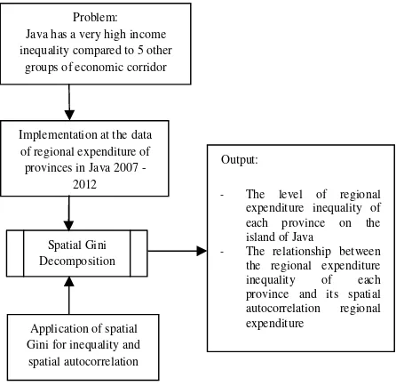
This research aims to (1) calculate the level of regional expenditure inequality of each province on the island of Java; (2) find the province having greatest contribution to expenditure inequality on the Island of Java; and (3) determine the relationship between the inequality of the province referred to in point 2 and its spatial autocorrelation of regional expenditure. After processing using spatial Gini decomposition method, the results show that (1) the level of regional expenditure inequality of each province can be seen in Table 1; (2) province of Banten was the province having greatest contribution to regional expenditure inequality on the Island of Java, (3) eventhough Banten is the province which was almost always the highest in regional expenditure inequality in Java, there is no indication of significant spatial autocorrelation of regional acceleration of economic growth, equitable distribution of income inequality, and poverty eradication (Todaro, 2007). Income inequality is a problem that arises because of uneven economic development. This is due to the difference in income between the rich and the poor.
Economic growth starts from a pre-industrial to industrial, results in an increase in the gap, and then will be stable for a while and then the gap will be decreased (Kuznets, 1995). The same was found by Adelman and Morris (1973), who stated that the rapid economic grow is always followed by the increasing gap, especially in the early stages of economic development process. Hence, measurement of inequality based on the distribution of income is required.
Statistics Indonesia, or abbreviated as SI, in 2008, explained that the calculation of inequality that is often used is the Gini coefficient. Gini coefficient meets the criteria: 1) does not depend on the value of the average (mean-independent); 2) does not depend on the total population (population size independent); 3) symmetrical; and 4) Pigou-Dalton transfer sensitive.
data is required. The other side, Rey and Smith (2013) found a Gini coefficient calculation technique that is decomposed to obtain the magnitude of inequality in one region and how to measure spatial autocorrelation that occurs among neighboring sub-regions within the region. Rey (2004) also stated that the measure of income inequality and spatial autocorrelation has a strong positive relationship.
Analysis of inequality in Indonesia in 2008 - 2014 was conducted by Devianingrum (2014). Devianingrum grouped provinces in Indonesia into 6 groups based on economic corridors. In her analysis, Devianingrum stated that in the period 2008 - 2012 occurred a very high inequality between Java and 5 other groups. This was caused by the presence of a very large inequality that was seen from the level of income.
Based on the explanation above, it can be formulated how to analyze regional income inequality using the Gini spatial decomposition method in the economic corridor group of Java. We are interested in examining whether for each province on the island of Java experienced a very high income inequality. By using spatial Gini decomposition method, we want to know calculating the level of regional expenditure inequality of each province on the island of Java; (2) finding the province having greatest contribution to expenditure inequality on the Island of Java; and (3) determining the relationship between the inequality of the province referred to in point 2 and its spatial autocorrelation of regional expenditure.
II. Theoritical Review
This section consists of three sub-sections. The first subsection describes some terms that are important to support this research. The second one contains a brief description of previous studies related to spatial Gini coefficient. The third one contains a brief description of the coefficient values range from zero to one, where zero is perfect equality, meaning everyone has the same income. While one, perfect in equality, means that one person has all the income in the population and all the other people do not have anything. When adopted to the question of regional income inequality, observation units are geographically referenced. However, the Gini coefficient is a measure of inequality that is invariant in location, which gives an overall picture. Invariant in location implies that the Gini coefficient is not sensitive to the absolute and relative position of the values of observation on the map. Gini can inform us that the inequality is going on, but did not inform where inequality that occurred within the region (Silber 1989; Dawkins, 2006, 2004; Arbia 2001 in Rey and Smith 2013).
2.1.2. Income inequality inequality measure and spatial clustering measure, the classic Gini coefficient turned out to contain the spatial autocorrelation measure. In this case, the decomposition of the Gini is pair wise disjoint and mutually exclusive. (Rey and Smith 2013)
2.1.4. Spatial weight matrix
autocorrelation), spatial structure, or spatial interaction (Daniaty, 2012). These three elements neighboring. SI (2013) defines the spatial autocorrelation as a representation of the regional association in general. Spatial autocorrelation is due to the interaction among the regions. This interaction states that the value of the observation in a region affected by the value of the considering neighborhood. The results of this research are a decomposition of Gini coefficient into two components – neighbor and non-neighbor components; and a spatial Gini test for spatial autocorrelation. Rey and Janikas (2006) have developed an application for Spatial Gini, named STARS: Space-Time Analysis of Regional System. Devianingrum (2014) developed application for calculating spatial Gini coefficient and testing a spatial autocorrelation. The spatial application has been tested to real data of per capita expenditure in Indonesia from 2008 until 2012. The conclusion was that there was a significant income inequality in Indonesia when viewed by the group of economic corridors. In this case, the group of economic corridors Java provided the largest contribution to the inequality in Indonesia.
2.3. Framework
Framework of this research can be seen in Fig. 1.
III. Methodology
The methodology consists of data sources and tools, and research methods.
3.1. Data Source and Tools
Trial data used in this research is from Statistics Indonesia (abbreviated as SI), based on the National Socioeconomic Survey (SUSENAS) 2007-2012. In Indonesia, data of income per capita are not available, so that the data used are data of household expenditure which were obtained from Susenas. Data of household expenditure were processed, resulting in data of average expenditure per capita of a regency/city, here in after referred to as the data of regional
expenditure. We use this regional expenditure variable as an approach to the average income of a regency/city. Application used to perform calculations is WIRES 2.0.
3.2. Research Method
The method used in this research is based on a method developed by Rey and Smith (2013). To test the spatial autocorrelation, we use Monte-Carlo simulation. The Gini based test for autocorrelation is defined as:
where:
is the value for variable x observed at region i = 1, 2, …, n. ̅= ( 1/ )∑ .
, is an element of a binary spatial weights matrix expressing the neighbor relationship between region i and j.
= ∑ ∑ ,
̅ +
∑ ∑ ,
̅ .
SG can be interpreted as the share of overall inequality that is associated with non-neighbor pair of locations. Inference on this statistics relies on random spatial permutations of the data. More specifically, the value of (1) is first obtained from the original data. Next the values are spatially permuted to simulate spatial randomness and the test statistic is calculated for this new map pattern. Additional permutations are carried out and the original value of the statistic is then compared to the distribution of values obtained from the randomly permuted data. The pseudo p-value for the observed test statistic is then defined as:
where C is the number of the M = 499 permutation samples that generated SG values that were as extreme as the observed SG value for the original data. The definition of extreme depends on whether one is conducting a one or two-tailed test. In the former a directional test holds in which case the alternative hypothesis is that there is positive (negative) autocorrelation and values of the test statistic that exceed (are less than) the observed value from the original example contribute to C. (Rey and Smith 2012)
The algorithm for calculating the spatial Gini coefficient and for testing spatial autocorrelation, can be seen in the flowchart below
DATA START
END Cal cula te w eigh t
Gr ou p?
Re calculat e w eigh t f or Gini Spat i al
Cal cula te Gin i Spa tia l Com po nent 1
Cal culat e p se udo p-value Cal cula te Gin i Spa tia l Com po nent 2
[Yes] [No]
IV. Results and Discussion 4.1. Expenditure Inequalities
Table 1 shows that the greatest in equality was almost always suffered by the province of Banten, as shown by the Gini coefficient. Only in 2010, the Gini coefficient of Province of Banten was in the second position, under Jakarta. This means that, Banten experienced income inequality which was quite large compared to other provinces in Java. While in Province of Central Java, the income inequality was still relatively low.
It was also the case in 2008, where the province of Banten was a province that had a fairly high income inequality, with a gini coefficient of 0.4200, and the lowest was also the province of Central Java. There was little difference in the year 2009, in which inequality was lowest in the province of East Java, whose gini coefficient was 0.1611.
In 2010, the greatest inequality occurred in DKI Jakarta, with a Gini coefficient of 0.2314 and the lowest inequality occurred in the province of West Java, with a Gini coefficient of 0.1541. Inequality in Province of Banten was still high, which is the Gini coefficient of 0.2067.
In 2011, the province of Banten ranked highest in terms of income inequality, with a value of 0.2067, while the Province of Central Java ranked lowest, with a value of 0.1343. In 2012, the province of Banten also still ranked highest in terms of income inequality, with a value of 0.2066, while DKI Jakarta was ranked lowest in Java, with a value of 0.1119.
So it can be concluded that the share of inequality in Java was mainly derived from province of Banten. Inequality between groups of the poor with the groups of rich was very high. This was in line with research that had been done by Devianingrum (2014) which stated that Java is a group of economic corridor has the highest inequality in comparison with groups of other economic corridors.
Once traced, Province of Banten had the largest share compared to five other provinces in Java. The smallest contribution to the province alternated annually.
Table 1. Gini coefficient by Province in Java 2007 – 2012
Next section explains the spatial autocorrelation of each province.
4.2. Analysis of Spatial Autocorrelation
Data of average expenditure per capita per province on the island of Java from 2007 to 2012 are shown in Fig. 2. The figure shows that the average expenditure per capita in Province of DKI Jakarta from 2007 to 2012 was ranked first, followed by Banten. While for other provinces,their own average expenditure were still relatively the same.
When we view the growth of GDP at constant prices 2000 of each province in Java, as seen as in Fig. 3(a), the GDP of DKI Jakarta in 2007-2008 were still under the province of West Java. But slowly, in the years 2009 - 2012 Jakarta showed significant GDP growth compared to the other provinces in Java. It can be seen from Fig. 3(b) that in the DI Yogyakarta, from 2007 to 2012, the growth of GDP was slower than the other provinces in Java.
Figs. 4 shows that each spatial Gini coefficient of West Java is the sum of its neighbor component and non-neighbor component. 2007 was a year in which income inequality was very large compared to the subsequent years. In 2011-2012, inequality increased, whereas before, namely in 2008-2010 inequality had decreased and fluctuated. For example, at Capita 2007 in Fig. 4(b), the neighbor component is 0.0086, while the non-neighbor component is 0.2067. If the two are added together, the result is equal to 0.2153, which is equal to the classical Gini coefficient or spatial Gini coefficient.
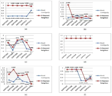
Based on Fig. 5(a), all p-values yielded are above 0.1. This means that for Province of DKI Jakarta, there is no significant spatial autocorrelation when using both of the weights. This may be due to the relatively small number of regencies/cities in Jakarta. If seen from the graph, rook contiguity weight has much lower p-value compared to another one. From Fig. 5(a), there are some p-values equal to 1 when using 3-nearest neighbors. This indicates that there is no significant spatial autocorrelation, neither positive nor negative.
Fig. 5(b) shows the different results compared to those of Province of DKI Jakarta. Based on Fig. 5(b), p-values of spatial gini test for spatial autocorrelation using rook-contiguity weight are smaller than those using 3-nearest neighbors weight in 2007, 2010 and 2011. In this case, the autocorrelation that happened was positive autocorrelation. There was indication of positive spatial autocorrelation significantly among regencies/cities in West Java. This implies that the neighboring regencies/cities tend to form clusters, where clusters are formed can consist of regencies/cities that have lower regional expenditure together, or on the contrary, have a high regional expenditure together.
were no significant spatial autocorrelation in the province of Central Java, either using rook contiguity weight or 3-nearest neighbors weight.
Fig. 5(e) shows that from the four weights, it turns out that rook contiguity weight has a value below 0.1 in almost every year in East Java – except in 2009. However, in 2012, the p-value is close to 0, when using both of the weights. When we use the rook contiguity weight, there was a significant positive spatial autocorrelation among regencies/cities. When we use the 3-nearest neighbors weight, there was no significant spatial autocorrelation among regencies/cities in East Java.
For provinces of Banten and D.I. Yogyakarta, based on Fig. 5(d) and 5(f), the results of the spatial gini test for spatial autocorrelation were quite similar to those of province of DKI Jakarta, that has been explained previously, i.e. there is no significant spatial autocorrelation when using both of the weights. This may be due to the relatively small number of regencies/cities in both provinces respectively.
V. Conclusions and Suggestions 5.1. Conclusions
Based on the objectives to be achieved in this research, the conclusions obtained are as follows:
1. The level of regional expenditure inequality of each province can be seen in Table 1.
Banten. Almost every year from 2007 until 2012 Banten’s Gini coefficient was the highest compared to other provinces on the island of Java.
3. Eventhough Banten is the province which was almost always the highest in regional expenditure inequality in Java, there is no indication of significant spatial autocorrelation of regional expenditure.
5.2. Suggestions
Suggestions can be presented for this research are as follows:
1. This method should be tested for other variables, such as socioeconomic variables, to see how much inequality in a region that is affected by the surrounding regions.
2. For provinces having a small number of regencies/cities, to be more careful in determining the weights matrix.
3. Compare test results for spatial autocorrelation using spatial Gini with those using Moran I. 4. Try to use the other weights that are more relevant to know the spatial autocorrelation of
regions experiencing inequality.
Bibliography
[1] Adelman, I., Morris, C. T.: Economic Growth and Social Equity in Developing Countries. Stanford University Press, Stanford (1973)
[2] Daniaty, D.: Module Development of Spatial Weights for Spatial Analysis Applications. Institute of Statistics, Jakarta (2012)
[3] Devianingrum, H.: Spatial Gini Decomposition in Indonesia Years 2008-2011. Institute of Statistics, Jakarta (2014)
[4] Glaeser, E. L.: Inequality. NBER Working Paper. 11511 (2005)
[5] Goodchild, M.: Spatial Autocorrelation. CTMOG – Concepts and Techniques in Modern Geography. University of Western Ontario, Ontario (1986)
[6] Kuznets, S. S.: Economic growth and income inequality. American Economic Review.
45(1), 55-65 (1955)
[7] Rey, S. J.: Spatial analysis of regional income inequality. In: Goodchild, M., Janelle, D. (eds.) Spatially Integrated Social Science: Examples in Best Practice, 280–299. Oxford University Press, Oxford (2004)
[8] Rey, S. J., Janikas, M. V.: STARS: space-time analysis of regional systems. Geogr. Anal.
38(1), 67–86 (2006)
[9] Rey, S. J., Smith, R. J.: A Spatial Decomposition of the Gini Coefficient. Lett Spat Resour Sci. 6, 55–70 (2013)
[10]SI.: Analysis and Calculation of Poverty Level in 2008. SI, Jakarta (2008)
[11]___.: Spatial Analysis of Population Indonesian Life Expectancy Based on Results of the Population Census 2010. SI, Jakarta (2013)