IMAGE-BASED TOPOGRAPHY RECONSTRUCTION BY MINIMIZING THE
REPROJECTION-ERROR OVER A SURFACE
Shalev Mor, Sagi Filin
Mapping and Geo-Information Engineering
Technion
–
Israel Institute of Technology, Haifa, Israel
(filin,shalevm)@technion.ac.il
Commission III, WG III/4
KEY WORDS: Surface reconstruction, Surface Evolution, Photo-consistency, Reprojection-error Minimization
ABSTRACT:
Image based three dimensional modelling of small scale scenes sees an increased demand in recent years due to algorithmic advances, and growing awareness of users to the value of scene documentation in three dimensions. Nonetheless, most of the reported image-based reconstruction methods are either point driven, relying on matching large set of automatically sampled points (e.g., SIFT, SURF), or integral approaches. The latter are commonly based on generating an entire map of matching. For many such stereo-correspondence methods, however, images which are acquired from a narrow baseline and similar orientations are usually needed, in order to ensure satisfying results. We present in this paper a reconstruction approach, assuming both visibility and Lambertian reflectance, which is intended to be less affected by image difference. The proposed method performs a surface evolution which is implemented by an iterative scheme, applying a gradient flow which minimizes a reprojection-error cost function. The algorithm is applied on scenes of complex topography and varied terrain. Our results show applicability of the method, along with its satisfactory performance for some difficult imagery configurations.
1. INTRODUCTION
Detailed three dimensional mapping of small scale scenes sees an increased demand in recent years. This trend can be attributed to increasing computing power, graphic hardware, and technological and algorithmic advances. It has also been thriving by growing awareness of users to the value of scene documentation in three dimensions, such as visualization, scene analysis, and more.
Among the various data acquisition techniques, the most effective ones for geographical scenes reconstruction are based on laser scanning technology and images. Although laser based point-clouds provide a dense set of data for scene description, limited availability of scanners and their prohibitive cost makes them not as widely applied as may be anticipated. In contrast, low cost cameras are far more available, and enable 3D modelling which is less costly, and in many cases generate data that are more detailed. Consequently, image-based 3D modelling is still relevant nowadays (Remondino and Menna,
2008). Image based methods for three-dimensional
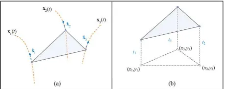
reconstruction, are often motivated by photo-consistency criteria. Most of the reported approaches for environmental and geographical scenes are point driven, and rely in many cases on the detection and matching or a large set of points (e.g., using the SIFT or SURF operators) (Remondino and El-Hakim, 2006; Barazzetti et al. 2010). Traditional methods for integral scene reconstruction are stereo-vision based and generate disparity-maps which match each image pixel to a counterpart in the other image (Figure 1a). Generation of such maps is often subjected to an optimization scheme of some energy function, e.g., graph-cuts, belief-propagation and so forth (Scharstein and Szeliski, 2002; Brown et al., 2003). Notwithstanding, implementation is usually carried out in image-space, and is subjected to its resolution and precision, whereas the final reconstruction model is given in three-dimensional space. Moreover, these methods seem ineffective for wide baselines or significant orientation differences. Therefore, they may turn less
applicable in complex natural environments which contain varied topography along with discontinuity and unsmooth features therein (Mor and Filin, 2009).
A somewhat different approach for 3D modelling is surface evolution (Faugeras and Keriven, 1998, Gargallo et al, 2007, Delaunoy and Prados, 2011) which often generates a model which minimizes the images reprojection-error objective function (also known as energy or cost function) (Seitz et al., 2006). This minimization is based on the assumption that the intensity image values of the same object-space point should share similar values; more realistically, have a minimal intensity difference between them. The process begins with an initial coarse approximated surface, and in each iteration the surface should change or "evolve" by some criteria until convergence to the optimal solution (by minimizing an objective function) is reached.
Following such approaches, this paper proposes a methodology for three-dimensional surface reconstruction of a textured scene, which is motivated by photo-consistency, assuming visibility and Labertian reflectance. Our objective is to generate an explicit digital surface model (DSM) based on minimization of the integral reprojection-error generated by an image-set over the surface. An initial coarse surface is evolved iteratively using the gradient of a reprojection-error energy function (gradient-descent method). Contrary to traditional reconstruction methods, our approach is surface-based (Figure 1b) and advancement is computed in three-dimensional model-space. The advantages of the proposed approach over traditional ones lie in the fact that the surface reconstruction is generated in a three-dimensional model space which makes it less subjected to image resolution. Moreover, since no point- or pixel-direct matching is required, the use of image sets with wide baselines and significant difference in their orientations becomes possible and in a more effective manner. The paper presents a theoretical scheme, along with an implementation for a triangular mesh model. Modification to other explicit surface representations is, however, straightforward.
The organization of this paper is as follows: we first introduce the main concept of the surface reconstruction as casted by an energy minimization. Section 2.1 develops expressions for the energy function gradient which enables to evolve the surface. Section 2.2 elaborates on computational aspects which enable us to implement our method for digital images. Section 3 demonstrates the application of the method on an archaeological site that offers complex topography including varied terrain, discontinuities and unsmooth features therein. The results show applicability of the method, along with its satisfactory performance for difficult imagery configurations. The paper concludes with summary and discussion.
Figure 1. Illustration of 3D point determination by a one-dimensional search, a) an image-space search along the epipolar line using the radiometric information directly, b) the search is along the vertical locus, and the radiometric values are obtained by projection to image-space. The positioning in both cases is motivated by requiring minimal values for the intensity differences.
2. SURFACE RECONSTRUCTION
Our surface reconstruction approach is based on minimizing the reprojection-error in the three-dimensional object space. In order to do so we first describe the reprojection-error as a scalar field over the 3 Euclidean domain. For simplicity we focus in first on an image pair alone, but the expansion to multiview configuration is relatively straightforward by adding terms for all image pairs.
Consider two images of a specific scene: a reference image I and a target image I'. Every object-space point x|=|[x,y,z]T can be projected into each one of the images, and retrieve the intensity value Ȋ(x) and Ȋ'(x). Notice that here Ȋ: 3→ is a function over a point in the three-dimensional object-space (as opposed to I(u,v) which is the intensity function for a two-dimensional image-space point). The relation between the two is Ȋ(x) = I(P(x)), where P: 3→ 2 is the projection of the object-space coordinate onto the image. We can now define the reprojection-error scalar field as the square difference of intensity values as given in Eq. (1)
2( ) ( ) ( )
Dx I x Ix (1)
This scalar field may be calculated for any point in the field-of-view of both images. Figure 2 provides a graphic illustration of such a field.
We would like to find a surfaceΓ which represents the scene optimally, i.e., a surface that would maintain photo-consistency, or minimize the reprojection-error. As our interest is in an integral solution for the entire surface, our objective would be minimizing the cost function given in Eq. (2):
2( ) ( )
E I I d
x x (2)where dσ is the differential surface area element. This is an integration of the reprojection-error field D(x) over the surface
Γ. Using continuous surface representation the optimization can be formulized as a variational problem. However, we can also use a discrete surface representation, such as Triangular Irregular Network (TIN) mesh or Digital Terrain Model (DTM) grid. In such a case, the surface would be represented by a set of piecewise functions (planes for TIN, bilinear or bi-cubic for grid etc.) where each of them depends on some finite number of parameters:
1
2
[ ,..., ] 1
min ( ) ( )
T
nP k n
t t k
I I d
tx x
(3)
The choice here is of a triangle-mesh representation, and so, the integration is over a set of triangles {Tk, k = 1,2,…,nT}, and the solution is of a finite vector of npz-ordinate [t1,t2,…,tnp].
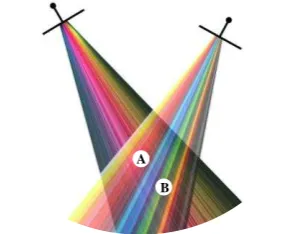
Figure 2. Illustration of the reprojection-error field. Region A is of low reprojection-error as its projection color in both images is red. On the other hand, the reprojection-error of region B is high due to the collision between red and green colors of its image projection.
Our choice of solving this optimization problem is by using the gradient-descent method. Using it we should calculate the gradient of the objective function given in Eq. (3), i.e., its vector of derivatives with respect to the z-ordinate [t1,…,tnp] of each of the vertices (Figure 3). The update for each iteration q should be tj(q+1)#=#tj(q)#–#α
j
E t
for some scalar step of size α .
Figure 3. A surface (left) and the gradient of its vertices (right) visualized by the arrows.
2.1 Gradient of the Energy function
The objective energy function introduced in Eq. (3) is in fact an integral over the entire surface, and therefore depends on the parameters ti. As these parameters change, the surface evolves. Notice that the domain of integration changes as well as the energy function value. This concept of a surface flow according to some direction, which is the gradient in our case, is
A
A
A
B
sometimes related as gradient flow (Delaunoy and Prados, 2011).
To illustrate the flow, consider a surface that depends on a single parameter, t, termed in the following as time, for traditional reasons. For simplification of the mathematical derivation, we restrict our surface to a single triangle. Our energy function is an integration of some scalar field over the surface.
2.1.1 Time Derivative for a Single Triangle
Consider a triangle T in 3D-space, defined by its three vertices
xi|=|[xi,yi,zi]T, i=1,2,3. Let D: 3→ be some scalar field, then its integration over T may be expressed as a surface integral E. In order to introduce surface evolution or flow, we consider the triangle surface as moving in time in such a way that its three vertices move along some time dependent curves (Figure 4a). Consequently, the domain of integration also depends on time, and thus can be written as:
dependent, computing the derivative dE/dt is not a trivial task. Thus we should use the Leibniz integral rule for differentiation under the integral sign (Flanders, 1973). To overcome this difficulty we may transform the domain of integration into a 2D coordinate system for which it has no time dependency. This is done by changing the surface domain to the unit triangle in 2 (5). Since now the domain of integration is not time dependent, we may derive it and obtain the expression in Eq. (6).
computed only using the triangle vertices it does not depend on the integration parameters r and s, and therefore can be taken outside of the integral, which leads to the following expression for the derivative normal vector of the triangle.Figure 4. a) a general time dependent triangle surface model, b) an explicit triangle surface model .
2.1.2 The Derivative for an explicit TIN model
As we have chosen to use an explicit triangular mesh for a surface representation, the shape of the surface is determined by the z-ordinates of the triangles vertices (Figure 4b). For a single triangle Tk, the energy Ek which is integrated over it, depends only on a limited (three) set of parameters, tj, which correspond to its three vertices. The gradient of our energy function, is therefore a vector containing the derivatives of the energy E(t1,..,tnp) with respect to the values tj of each vertex
j|=|1,2,…,np, where np is the number of vertices. Using Eq. (7) the j-th component of the gradient may be expressed by
2
For a single triangle Tk, and without any loss of generality, we name these three parameters t1,t2,t3, which correspond to the ISPRS Annals of the Photogrammetry, Remote Sensing and Spatial Information Sciences, Volume I-3, 2012
Continuing with an expression for D, the reprojection-error
where Ȋ and Ȋ' are the aforementioned 3D color fields generated by the reference and target image respectively. Deriving this color field function in 3D space is not as obvious, and so we use the 2D image function which generates it by the relation using the projection matrix P3×4:
~ expressed by the Jacobian matrix
11 31 12 32 13 33
We can now write explicit expressions for the derivatives of E. Prior to that we note that the vectors we obtained for ẋ in Eq. necessary derivatives of E.
challenging task. Although the 3D function Ȋ(x) is theoretically well defined, it is difficult to implement it practically. Eq. (19) would be entirely computable in the reference image-space (u,v) had it not included the term I'(u') which is the actual target image-space. Therefore, in order for the integrand to be a function of single image-space domain (u,v), we have to reproject the target image coordinates (u',v') onto the reference image. Since the two projection functions are defined by u=P(x) and u'=P'(x), we may determine that u'|=|P'(P-1(u)). This composite function may seem indefinite, since we cannot trivially transform image coordinates from one to the other (by inverting P). However reprojection may be computed using the surface data. Taking the surface into consideration we can intersect a reference image ray generated by an image point, leading to a 3D object-space point, which can be then projected to the target image. A geometric illustration of such reprojection is given in Figure 5.
We now define the reprojected image function
Ĩ(u)|=|I'(u')|=|I'(|P'(P-1(u))|), which may be constructed by the original target image I', the two perspective projection matrices of both images, and the surface. Notice that the reprojected image is a synthetic one created by first inversely-projecting the target image onto the surface, and then projecting it from the surface to the reference image-space. Using the above notations we may now write Eqs. (3) or (19) as:
is the coefficient of the surface area element in the image-space, which is developed in the Appendix. As Eq. (21) shows, J depends on the image-space point u|=|[u,v]T, its inversely ISPRS Annals of the Photogrammetry, Remote Sensing and Spatial Information Sciences, Volume I-3, 2012
projected 3D object-space coordinates x|=|[x,y,z]T, the image perspective projection matrix P and the surface normal vector n
at this point. The value w|is p31x|+|p32y|+|p33z|+|p34.
Figure 5. Illustration of an image-pair reprojection.
Applying the reprojection approach we can now write the following expression for integration of Dz. Using Eqs. (17) and (20) we may write
1,3 3,3 2,3 3,3
1,3 3,3 2,3 3,3
( )
( )
2
2
z
P
P
u v
u v
p p u p p v
w w
p p u p p v
w w
D d I I I I J du dv
I I I I J du dv
T T
T
(22)
which transforms the domain of integration from the 3D surface in object-space into both the reference and target image-spaces. Here Ĩ' is the inverse reprojected image from the reference to the target one, and J' is the coefficient for the target image. This enables us to compute the gradient of our energy function, and therefore perform a surface evolution in that direction. We detail here the algorithm for evolving an initial course surface based on minimization of the reprojection-error accumulated of an image pair of the scene.
#1 input:
#2 two images I and I'
#3 set of triangles Ti, i = 1,2, …, nT
#4 initial set of vertices xi, yi, zi = ti, i = 1,2, …, np
#5 output:
#6 final values for the z-ordinates ti, i = 1,2, …, np
#7 routine:
#8 assign E = 0 /* energy */
#9 define the gradient vector E of np elements and assign them to 0
#10 for each triangle Tk, k = 1,2,…,nT
#11 compute the values g1,g2,g3,g0 for the triangle
#12 compute the triangle normal n1,n2,n3
#13 project all the triangle vertices coordinate on the image I
#14 for each pixel (u,v) in the image I
#15 find the triangle Tk containing the pixel (u,v)
#16 assign t1,t2,t3 to be the indices of the vertices of Tk
#17 compute the surface point x,y,z (by intersection)
#18 compute J using Eq. (21)
#19 compute uz and vz using Eq. (16)
#20 compute the numerical derivatives Iu and Iv of image I at (u,v)
#21 compute u',v' by projecting x,y,z on image I'
#22 assign D = ½[ I(u,v) – I'(u',v') ]2
#23 assign Dz = [ I(u,v) – I'(u',v') ][ Iu uz + Iv vz ]
#24 assign E0 = DJ , E1 = xDzJ , E2 = yDzJ , E3 = zDzJ
#25 assign E = E + E0
#26 compute additions to the three gradient components ∂E/∂t1, ∂E/∂t2, ∂E/∂t3 using Eq.(18)
#27 repeat the actions in rows #13-#26 while swapping I and I'
#28 for each vertex i = 1 to np
#29 assign ti = ti + α∂E/∂ti /* for some step-size α */
The computation of the surface point (x,y,z) in line #17 of the algorithm can be done by intersection of the ray line, generated by the image pixel and the camera exposure point, and the triangle plane. Moreover, the image derivative Iu and Iv in line #20 has to be computed numerically by using, for example, a gradient kernel. This can be done as a preliminary stage since the images do not change between iterations.
3. RESULTS
The proposed surface reconstruction method has been applied for scenes within an archaeological excavation site. It is demonstrated on a documentation project in Oren cave in the Carmel mountain ridge, as part of on-going research studying the origins and use of Manmade-bedrock-holes (MBH) in those sites. An excavation campaign performed in June 2011 serves as the case study here. Images were acquired during the excavation with a Nikon D70 camera, with 48mm Nikkon lens.
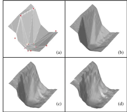
We focus here on the reconstruction of a 3D surface model of MBH embedded within rough topographic settings. The input images were taken from a distance of approximately 1.5m from the MBH, such that the baseline is ~80cm, with a large orientation difference (Figure 6). The computation is generated by a few manually sampled points for producing the initial coarse surface (Figure 6). The initial surface can be seen in Figure 7a.
(a) (b)
Figure 6. Images used for the reconstruction, along with sampled points for generating the initial coarse surface.
(a) (b)
(c) (d)
Figure 7. Stages of the surface evolution process, with the initial coarse surface in (a).
As noted the surface evolution is implemented by an iterative scheme, applying gradient flow on the z-ordinates of the vertices. Selected stages of the evolution are presented in Figure 7, and the final resulted surface is presented Figure 8a. ISPRS Annals of the Photogrammetry, Remote Sensing and Spatial Information Sciences, Volume I-3, 2012
Results show a complete and successful reconstruction of the surface enabling also to depict fine details that reflect its formation. Application of the proposed model to other MBHs has proven successful as well.
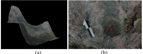
The reconstruction has been compared to existing methods as well. Use of the same images for reconstruction using the graph-cuts method has failed in the reconstruction completely (Mor and Filin, 2009). It seems that these methods which are based on disparity map in image-space tend to give inadequate results for poorly textured scenes, and seem to fail when the imaging configuration is of wide-baselines and is characterized by significant orientation difference. Furthermore, applying the SIFT algorithm on the images has yielded a sparse set of points, most of them are on the outer surface of the MBH and are insufficient to reconstruct the object successfully (Figure 8b). Here again, texture, and the wide baseline and orientations have a significant effect on the outcome.
(a) (b)
Figure 8. The reconstructed surface with texture in (a), whereas for comparison, a set of match points generated by the SIFT algorithm is presented in (b).
4. CONCLUSION AND DISCUSSION
This paper has presented a method for 3D reconstruction by surface evolution based on an image-pair, by employing a gradient flow for minimization of the reprojection-error. Additionally, an implementation scheme on a TIN mesh has been presented, and applied for complex topographic scenes. The results have shown applicability of the method, along with its satisfactory performance for some difficult imaging configurations. Future work may deal with expanding the accurate tie points for automated pose estimation of close-range
blocks. ISPRS The International Archives of the
Photogrammetry, Remote Sensing and Spatial Information Sciences, Saint-Mandé, France, Vol. XXXVIII, Part 3A, pp. 151-156.
Brown, M. Z., Burschka, D., Hager, G. D., 2003. Advances in computational stereo. IEEE Trans. on Pattern Analysis and Machine Intelligence, 25(8), pp. 993-1008.
Delaunoy, A., Prados, E., 2011. Gradient flows for optimizing
triangular mesh-based surfaces: applications to 3D
reconstruction problems dealing with visibility. Int. Journal of Computer Vision, 95(2), pp. 100-123.
Faugeras, O., Keriven, R., 1998. Variational-principles, surface evolution, PDEs, level set methods, and the stereo problem. IEEE Trans. on Image Processng, 7(3), pp. 336–344. Flanders, H., 1973. Differentiation under the integral sign. The
American Mathematical Monthly, 80(6), pp. 615-627. Gargallo, P., Prados, E., Sturm, P., 2007. Minimizing the
reprojection error in surface reconstruction from images. In
Proc. Of the Int. Conference on Computer Vision 2007, Rio de Janeiro, Brazil, (on CD-ROM)
Mor, S., Filin, S., 2009. Analysis of imaging configuration effect on surface reconstruction of complex sites. In Proc. of FIG working week 2009, Eilat, Israel, (on CD-ROM).
Remondino,|F., El-Hakim,|S., 2006. Image-based 3D modelling: a review. Photogrammetric Record, 21(115), pp. 269-291. Remondino F., Menna, F., 2008, Image-based surface measurement
for close-range heritage documentation. The International Archives of the Photogrammetry, Remote Sensing and Spatial Information Sciences, Beijing, China, Vol. XXXVII, Part B5, pp. 199-206.
Scharstein, D., Szeliski, R., 2002. A taxonomy and evaluation of dense two-frame stereo correspondence algorithms. Int. Journal of Computer Vision, 47(1-3), pp. 7-42.
Seitz, S. M., Curless, B., Diebel, J., Scharstein, D., Szeliski, R., 2006. A comparison and evaluation of multi-view stereo between the image-space coordinates (u,v) and the object-space 3D coordinates (x,y,z) can be stated by the following three
where the first two equation are variation of the co-linear law of Eq. (15), and the third one is the triangle plane equation in the 3D object-space. Deriving these three equations with respect to u and v gives
These two sets of equations may be written as