Directory UMM :Data Elmu:jurnal:J-a:Journal Of Economic Dynamics And Control:Vol24.Issue5-7.Jul2000:

(1)

q

I wish to thank Professors W.A. Brock, W.D. Dechert, K. Guler, K.L. Judd, B. LeBaron, and J. Rust for their very helpful suggestions and assistance. Of course, none of them are responsible for any shortcomings of this paper.

E-mail address:akdeniz@bilkent.edu.tr (L. Akdeniz)

Journal of Economic Dynamics & Control 24 (2000) 1079}1096

Risk and return in a dynamic general

equilibrium model

q

Levent Akdeniz

Bilkent University, Faculty of Business Administration, 06533 Bilkent Ankara, Turkey Accepted 30 April 1999

Abstract

In this paper we examine the relationship between risk and return on productive assets using the intertemporal general equilibrium model of Brock (1982, Asset Prices in a Production Economy, the University of Chicago Press, Chicago, pp. 1}42) as a basis for a simulation study. Current computational techniques are used to solve the growth model of Brock (1979, An Integration of Stochastic Growth and the Theory of Finance *Part I: The Growth Model, Academic Press, New York, pp. 165}192) in order to analyze the underlying"nancial model. Contrary to recent empirical"ndings, we"nd that there is a theoretical basis for the linear relationship between risk and return. This apparent contradiction is due in part to the fact that the dynamic relationship between risk and return depends on the level of output. ( 2000 Elsevier Science B.V. All rights reserved.

1. Introduction

Over the last two decades researchers have spent a great deal of time to evaluate the performance of the Capital Asset Pricing Model (CAPM) by testing how well the model"ts the data. The empirical evidence on the validity of the

(2)

CAPM is mixed. While some studies have concluded that the model is

misspeci-"ed others have found support for the predictions of the model. All of these studies, however encountered serious and di$cult econometric problems in their e!orts to provide the best empirical tests of the model. To what extent their results are derived by these methods has been a source of controversy. However, many researchers have taken the mixed empirical evidence to imply that the CAPM is not the correct model of risk and have attempted to test other determinants of expected stock returns. In this study, we examine the prediction of the CAPM, the linear relationship between risk and return, using the inter-temporal general equilibrium model of Brock (1982) as a basis for a simula-tion study. The dynamic structure of the model provides some insights about the dynamic relationship between risk and return which shed light on to the problems in empirical testing of the model. More speci"cally, we"nd that the dynamic relationship between risk and return depends on the level of output in the economy. In other words, the position of the economy on the business cycle matters in testing the relationship between risk and return.

Contradictory to the predictions of the CAPM, factors other than beta have been found to explain the cross-section of expected stock returns. These factors include market equity or in other words size (Banz, 1981; Reinganum, 1981), earnings price ratios (Basu, 1983), "rm's book value of common equity to its market equity (Rosenberg et al., 1985), and leverage (Bhandari, 1988). Recently, Fama and French (1992) reconsider these di!erent e!ects and"nd that size and book-to-market equity ratio provide the best characterization of the section of stock returns and conclude that beta does not explain the cross-section of expected stock returns. This empirical evidence has led researchers to deduce that the pure theoretical form of the CAPM does not agree well with reality. Although Fama and French (1992) make a persuasive case against the CAPM, their study itself has been challenged. Kothari et al. (1995) show that Fama and French (1992)"ndings are crucially contingent on the methodology and data used. Black (1993)"nds that the size e!ect, that is signi"cant in some periods, disappears in others; therefore, Fama and French's results may simply result from their select sample. Jagannathan and Wang (1996) show that the CAPM is able to explain the cross-sectional variation in average stock returns when betas and expected returns are allowed to vary over the business cycle and when human capital is included in measuring wealth.

(3)

1See Benhabib and Rustichini (1994) for a full description of a class of utility and production functions that have analytical solution.

asset-pricing theory. . . ..'. The reason researchers have taken this direction stems from problems that have been encountered in attempts to empirically verify the theoretical predictions of the CAPM.

Is it really the CAPM that is misspeci"ed or is it the empirical tests of the CAPM that are performed erroneously? The CAPM is a two-period, linear model expressed in terms of expected return and expected risk. Since these expectations cannot be measured, empirical studies use observed data to test for this linear relationship. However, in this study we are able to calculate both expected return and the true beta at a given period in time; thus, we are able to theoretically test the CAPM in its ex ante form. In such tests, we"nd that there is a linear relationship between beta and the expected return at any given period in time, as predicted by the CAPM. In addition, we have also found that the intercept as well as the slope of the Security Market Line shift up and down with

#uctuations in output in the economy, thereby suggesting that in the empirical tests of the CAPM, one needs to control for the#uctuations in the output level in order to properly test the model. In other words, in estimating the relation-ship between risk and return, only those observations that correspond to similar output levels should be used. Such"ndings gave us the impetus to pursue an empirical testing of the model using simulated data. We have performed two empirical tests of the CAPM. First, we have used the full data set (240 months) in Fama}MacBeth regressions (1973) of the cross-section of stock returns on beta and size (stock's price times shares outstanding). Second, we have controlled for the output level, therefore, used only those periods (20 months) that have output levels that are close to the mean output level. Without controlling for the output level, we have found that the size variable is signi"cant in explaining the cross-section of expected stock returns while beta is not. However, once we control for the output level the size e!ect vanishes and only beta remains signi"cant.

(4)

2Rouwenhorst (1995) provides a good review on this literature.

Prescott (1982) have used a quadratic approximation to the value function which also results in a linear policy function.2 Thus, these studies failed to produce the cyclical variation in equity premia.

The paper proceeds as follows: Section 2 presents the stochastic growth model of Brock (1979); Section 3 introduces the"nancial model; Section 4 presents the parameters and describes the simulation; Section 5 discusses the results; and Section 6 concludes the paper.

2. The growth model

The model we use as the basis for our study is the standard growth model with production, as speci"ed in Brock (1979). This is a model of economic growth with an in"nitely lived representative consumer. In this section, we heavily borrow from Brock and recapitulate the essential elements of the model:

max

where E is the mathematical expectation,bthe discount factor on future utility,

uthe utility function of consumption,c

tthe consumption at datet,xtthe capital stock at datet,y

tthe output at datet,fithe production function of processiplus undepreciated capital, x

it the capital allocated to process i at date t, di the depreciation rate for capital installed in processiandm

tthe random shock. Note thatf

i(xit,mt)"gi(xit,mt)#(1!di)xit, wheregi(xit,mt) is the production function of process i. For a description and interpretation of the model see Brock (1982). The"rst-order conditions for the intertemporal maximization are

u@(c

(5)

Since the problem given by Eqs. (2.1)}(2.6) is time stationary the optimal levels of

c

t,xt,xitare functions of the output levelyt, and can be written as c

t"g(yt), xt"h(yt), xit"hi(yt).

Our objective is to solve the growth model for the optimal investment functions,

h

i, to analyze the underlying implications of the asset pricing model.

3. An asset pricing model

The asset pricing model in Brock (1982) is much like the Lucas (1978) model. The main di!erence between these two models is that Brock's model includes production, thus by incorporating shocks into the production processes, it has the sources of uncertainty in the asset prices directly tied to economic# uctu-ations in output levels and hence in pro"ts.

The model is similar to the growth model in Section 2. There is one represen-tative consumer whose preferences are given in Eq. (2.1). On the production side there areNdi!erent"rms. Firms rent capital from the consumer side at the rate

r

itto maximize their pro"ts: n

i,t`1"fi(xit,mt)!ritxit.

Each"rm makes its decision to hire capital after the shock,m

t, is revealed. Here r

itdenotes the interest rate on capital in industryiat datetand it is determined within the model. Asset shares are normalized so that there is one perfectly divisible equity share for each "rm. Ownership of a share in "rm i at date

tentitles the consumer to the"rm's pro"ts at datet#1. It is also assumed (as in Lucas (1978)) that the optimum levels of asset prices, capital, consumption and output form a rational expectations equilibrium.

3.1. The model

The representative consumer solves the following problem:

max E

C

+=

(6)

3Note in this model market portfolio is e$cient, therefore Roll's critique does not apply. From the "rst-order condition (3.6) return on each asset satis"esu@(c

t)"bE[u@(Ct`1)Rit], which is the e$

cien-cy condition from the growth model. By summing Eq. (3.6) we get that the return on market portfolio also satis"es the e$ciency condition.

where P

it is the price of one share of "rm i at date t, Zit the number of shares of"rmiowned by the consumer at datetandn

itthe pro"ts of"rmiat datet.

The details of the model are in Brock (1982). The "rst-order conditions yielding from the maximization problem are

P

itu@(ct)"bEt[u@(ct`1)(ni,t`1#Pi,t`1)] (3.6)

and

u@(c

t)"bEt[u@(ct`1)fi@(xi,t`1,mt`1)].

We use these"rst-order conditions to get the prices for the assets. Brock (1979) shows that there is a duality between the growth model ((2.1)}(2.6)) and the asset pricing model ((3.1)}(3.5)), and the solution to the growth model is also solution to the asset pricing model. Once the solution to the growth model is obtained, the asset pricing functions can be solved for the prices for the assets by Eq. (3.6).

Since in equilibrium there is one share of each asset, the value weighted market portfolio is

and the dividends (pro"ts) are

n

Now, de"ne the return on each asset by

R

and the return on the market portfolio by3

R

(7)

Now de"ne the pro"t, consumption and output functions by

and the asset pricing functions by

P

i(y)u@(c(y))"bE [u@(c(>(y,m)))(Pi(>(y,m))#ni(y,m))].

Once we have the pricing functions we next de"ne the return functions

R

and the functions for the variances

p2

Solution to the growth model enables us to calculate above functions at di!erent output levels. Except for a very special case of the utility and the production functions, there are no closed form solutions for the optimal investment func-tions for the problem outlined in Eqs. (2.1)}(2.6). One must use numerical techniques in order to analyze the properties of the solutions to the asset pricing model. There are many di!erent methods to solve these types of problems. A wide variety of these methods are discussed in the special volume of the Journal of Business & Economic Statistics (January 1990). We have chosen to use the projection method in Judd (1992). The details of the solution are in Akdeniz and Dechert (1997).

(8)

Table 1

Production function parameters

State a h d State a h d State a h d

Firm 1 Firm 2 Firm 3

1 0.4530 0.1300 0.100 1 0.3410 0.2175 0.150 1 0.6060 0.1105 0.200 2 0.1950 0.1018 0.100 2 0.4290 0.0825 0.150 2 0.2740 0.1431 0.200 3 0.8900 0.0715 0.100 3 0.7060 0.1446 0.150 3 0.1900 0.1773 0.200 4 0.5530 0.0639 0.100 4 0.2130 0.2212 0.150 4 0.7610 0.2767 0.200

1 0.3570 0.1812 0.130 1 0.3490 0.1120 0.170 1 0.4578 0.1275 0.105 2 0.7430 0.1370 0.130 2 0.5290 0.2100 0.170 2 0.2160 0.1022 0.105 3 0.1160 0.0914 0.130 3 0.5370 0.0916 0.170 3 0.9000 0.0685 0.105 4 0.5880 0.1005 0.130 4 0.6920 0.1523 0.170 4 0.5578 0.0620 0.105

1 0.3327 0.2272 0.145 1 0.5962 0.1143 0.195 1 0.3618 0.1714 0.132 2 0.4241 0.0829 0.145 2 0.2642 0.1382 0.195 2 0.7527 0.1564 0.132 3 0.6914 0.1348 0.145 3 0.2094 0.1870 0.195 3 0.1403 0.0894 0.132 4 0.2227 0.2260 0.145 4 0.7561 0.2713 0.195 4 0.5636 0.1130 0.132

1 0.3499 0.1236 0.167 1 0.4672 0.1213 0.097 1 0.3565 0.2052 0.154 2 0.5288 0.1979 0.167 2 0.2038 0.1124 0.097 2 0.4109 0.0808 0.154 3 0.5351 0.0919 0.167 3 0.8961 0.0836 0.097 3 0.7142 0.1441 0.154 4 0.7018 0.1572 0.167 4 0.5540 0.0640 0.097 4 0.2324 0.2216 0.154

1 0.6230 0.1105 0.192 1 0.3715 0.1913 0.134 1 0.3392 0.1314 0.167 2 0.2788 0.1494 0.192 2 0.7381 0.1240 0.134 2 0.5289 0.1980 0.167 3 0.1900 0.1631 0.192 3 0.1138 0.0927 0.134 3 0.5170 0.0914 0.167 4 0.7464 0.2600 0.192 4 0.5787 0.4420 0.134 4 0.6919 0.1604 0.167

(9)

1 0.4579 0.1311 0.102 1 0.3531 0.2105 0.152 1 0.6224 0.1254 0.192 2 0.1871 0.1098 0.102 2 0.4326 0.0830 0.152 2 0.2896 0.1336 0.192 3 0.8994 0.0715 0.102 3 0.6979 0.1536 0.152 3 0.1766 0.1670 0.192 4 0.5335 0.0626 0.102 4 0.2051 0.2102 0.152 4 0.7778 0.2567 0.192

1 0.3497 0.1304 0.122 1 0.3324 0.1072 0.174 1 0.4544 0.1202 0.104 2 0.7281 0.0949 0.122 2 0.5348 0.2034 0.174 2 0.1764 0.1215 0.104 3 0.1288 0.1004 0.122 3 0.5610 0.0939 0.174 3 0.8953 0.0705 0.104 4 0.5756 0.1227 0.122 4 0.6908 0.1524 0.174 4 0.5448 0.0631 0.104

1 0.3325 0.2363 0.145 1 0.5914 0.1224 0.195 1 0.3570 0.1734 0.132 2 0.4422 0.0829 0.145 2 0.2657 0.1602 0.195 2 0.7507 0.1207 0.132 3 0.7152 0.1348 0.145 3 0.1965 0.1658 0.195 3 0.1259 0.0932 0.132 4 0.2110 0.2202 0.145 4 0.7513 0.2601 0.195 4 0.5899 0.1111 0.132

Firm 25

1 0.3431 0.1281 0.167 2 0.5289 0.1985 0.167 3 0.5515 0.0908 0.167 4 0.6709 0.1440 0.167

L.

Akdeniz

/

Journal

of

Economic

Dynamics

&

Control

24

(2000)

1079

}

1096

(10)

4. Simulation

In this section we present a solution to the model for one set of parameter values. The speci"c model we chose to estimate is

u(c)"cc

c, f(x,m)"h(m)xa(m),

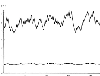
wherecis the utility curvature parameter. Campbell and Cochrane (1994) state that a utility curvature parameter of!1.37 matches the postwar US data, thus c"!1.37 is chosen for the utility curvature parameter. Unlike Campbell and Cochrane and other literature on habit formation, our results are derived with a constant utility curvature parameter. The value of the discount parameter,b, in yearly units is 0.97 and it is adjusted to monthly units. We solved the model for 25"rms using four equally likely states of uncertainty. All"rms use the same production technology. The parameters for the"rms are picked randomly and are reported in Table 1. The magnitude of the functions as well as the technical coe$cients are a!ected by uncertainty, thus both output levels and elasticities are subject to random shocks. Random shocks are independently and identically distributed. We have also simulated the economy with 240 realizations of the random shocks. To do so, we started with the mean output level of the ergodic distribution of the output as the initial level of output. Through the optimal investment functions, initial output is divided into consumption and investment. The computer then randomly chooses the state of the economy which gives forth the corresponding parameters for production. These parameters are used to determine the next period's output which is divided into consumption and investment at the beginning of the next period, and so on it goes. A problem with the iid shocks is that output#uctuates rapidly; therefore, the time series distribu-tion of output does not depict a typical business cycle output pattern. One needs to model a Markov process in the shocks to obtain the business cycle output pattern. Such a modi"cation is left for future research. In Fig. 1, we have plotted consumption and total output for 240 periods. Although output #uctuates rapidly, the consumption pattern is smooth over all periods which is consistent with observed data. In other words, this model replicates the typical pattern of widely#uctuating output levels and relatively constant levels of consumption over time.

5. Results

(11)

Fig. 1.

4Everywhere in this paper output level refers to economy-wide output level.

simulated data we are also able to test the empirical CAPM in its ex post form. Here, it is important to note that the simulated data is pure in the sense that it is not contaminated by any other e!ects. The data directly comes from the utility maximizing behavior of the consumer and the pro"t maximizing behavior of producers.

5.1. Theoretical results

(12)

Fig. 2.

theory. In particular they cite evidence that&. . . . equity risk premia seem to be higher at business cycle troughs than they are at the peaks'. They also add that

(13)

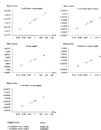
Fig. 3.

the troughs to the peaks of the business cycle are fully captured by Brock's model. As can be seen in Figs. 2 and 4, for a given beta and standard deviation, return and output level depict an inverse relationship. The intercept as well as the slope of the SML and CML change according to the#uctuations in output in the economy, thereby suggesting that empirical tests of the CAPM that average over long enough periods to include major portion of the business cycle may result in serious mistakes. In other words, in the empirical testing of the CAPM it is necessary to use those observations that correspond to similar levels of output in order to provide a proper empirical test of the model.

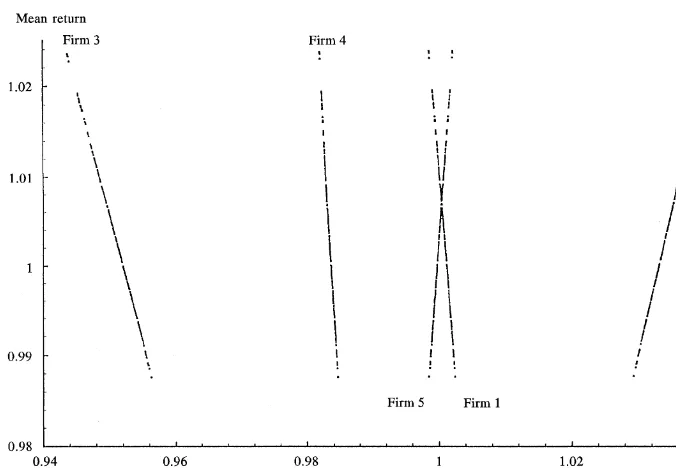
We have also plotted the relationship between expected return and beta for the"rst"ve"rms for 240 periods. Fig. 5 shows that some"rms get riskier as the output level increases while other"rms get less riskier. Although the true SML is positively sloped at any given period of time, it is possible to obtain a negatively sloped SML, if one uses time series averages in the estimations.

5.2. Simulated data results

(14)

Fig. 4.

5Mean output is 5.9 and the spread between peak and trough is 3.4. We choose those periods with 5.85("y

t("5.95, which comprises 3% of the spread.

(15)

Fig. 5.

Table 2

Average slopes from month-by-month regressions of stock returns on beta and size using the full (240 months) period

Univariate regressions Multivariate regressions

Beta Size Beta Size

9.667]10~4 3.486]10~6 5.931]10~4 4.517]10~6

(1.5769) (1.1724) (1.2091) (2.3684)

t-Statistics are in parenthesis. Since we have iid shocks, t-statistics are calculated assuming independence. Theset-statistics are t(c6

t)"c6t/(1/N)J+s2ctwhere c6tis the average of

month-by-month regression coe$cient estimates andsis the standard error.

the analysis. Empirical betas are estimated from a regression of monthly stock returns on the market portfolio. Since asset shares are normalized so that there is one perfectly divisible equity share for each "rm, the price of an individual stock is used for the size variable.

(16)

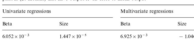
Table 3

Average slopes from month-by-month regressions of stock returns on beta and size using those periods (20 months) that have output levels close to mean output

Univariate regressions Multivariate regressions

Beta Size Beta Size

6.052]10~3 1.447]10~5 6.925]10~3 !1.046]10~5

(3.0064) (1.5183) (4.0976) (!1.4492)

t-Statistics are in parenthesis. Since we have iid shocks, t-statistics are calculated assuming independence. Theset-statistics aret(c6

t)"c6t/(1/N)J+s2ctwherec6tis the average of month-by-month

regression coe$cient estimates andsis the standard error.

stock returns. However, in the multivariate regressions, while empirical beta still remains insigni"cant, the size becomes signi"cant. The multivariate regression results are similar to those of Fama and French except for the sign on size.

We repeated the same test using the observations from only those periods whose output levels are close to the mean output level. Results are presented in Table 3. Both univariate and multivariate regression results show that the size e!ect vanishes and only beta remains signi"cant in explaining the cross-section of stock returns when we controlled for the output level. These results show that the CAPM is not misspeci"ed and suggest that it is necessary to use those observations that correspond to similar levels of output in the estimations in order to provide proper tests of the model.

6. Conclusion

In this study, we showed that a properly parameterized version of Brock's model provide a theoretical explanation of the observed #uctuations in asset prices. In particular, Brock's model provides a theoretical basis for the observed variations of the equity premia over the business cycles. Also, by using Brock's model, we have shown that the CAPM predictions hold in a fully dynamic general equilibrium framework. Particularly, we found a linear relationship between expected risk and expected return at any given period of time, which implies that beta is the sole determinant of the expected returns. Furthermore, from Fig. 1, the model (even with iid shocks) replicates the typical pattern of widely#uctuating output levels and relatively constant levels of consumption over time.

(17)

over the business cycle. This means that the empirical estimation of the SML, averaging over long enough periods to hold main portion of the business cycle, will result in serious errors. Thus, the empirical estimation of the SML must be done at similar levels of output. This phenomenon is further supported by Fig. 5, which indicates that, if the time series of returns are regressed on betas, one will get a much steeper relationship with the possibility of a wrong sign on the coe$cient.

In ongoing research, we examine various extensions and applications of Brock's model. Mainly, we model the shocks as Markov process in order to more closely approximate observed business cycle#uctuations of output. We also incorporate a growth factor to capture the trends in output. As further extensions to Brock's model, Black (1995, p. 159) suggests incorporating labour, adjustment cost of capital and human capital. Prescott (1982, p. 45) makes similar suggestions with regard to labour in order to more closely approximate the business cycle.

There are many potential applications of this model. It can be used to price assets other than those that are in Brock's two papers (1979, 1982). For example, by calculating the value of pure discount bonds, the term structure of interest rates can be determined over the business cycle. The dynamic implications of corporate tax policy can also be analyzed by using this model. It is our belief that with the advent in the use of simulation methods, the full richness of the applications of Brock's model can be developed.

References

Akdeniz, L., Dechert, W.D., 1997. Do CAPM results hold in a dynamic economy? A numerical analysis. Journal of Economic Dynamics and Control 21 (6), 981}1004.

Banz, R.W., 1981. The relationship between securities_' yields and yield-surrogates. Journal of Financial Economics 9, 3}18.

Basu, S., 1983. The relationship between earnings yield, market value, and return for NYSE common stocks: further evidence. Journal of Financial Economics 12, 129}156.

Benhabib, J., Rustichini, A., 1994. A note on a new class of solutions to dynamic program-ming problems arising in economic growth. Journal of Economic Dynamics and Control 18, 807}813.

Bhandari, L.C., 1988. Debt/equity ratio and expected common stock returns: empirical evidence. Journal of Finance 43, 507}528.

Black, F., 1993. Beta and return. Journal of Portfolio Management 20, 8}18. Black, F., 1995. Exploring General Equilibrium The MIT Press, Cambridge, MA.

Brock, W.A., 1979. An Integration of Stochastic Growth and the Theory of Finance*Part 1: The Growth Model. Academic Press, New York, pp. 165}192.

Brock, W.A., 1982. Asset Prices in a Production Economy. The University of Chicago Press, Chicago, pp. 1}42.

Campbell, J.Y., Cochrane, J.H., 1994. By force of habit: a consumption-based explanation of aggregate stock market behavior. National Bureau of Economic Research Working Paper d4995.

(18)

Fama, E.F., French, K.R., 1992. The cross-section of expected stock returns. Journal of Finance 47, 427}465.

Fama, E.F., French, K.R., 1993. Common risk factors in the returns on stocks and bonds. Journal of Financial Economics 33, 3}56.

Fama, E.F., French, K.R., 1995. Size and book-to-market factors in earnings and returns. Journal of Finance 50, 131}155.

Jagannathan, R., Wang, Z., 1996. The conditional CAPM and the cross-section of expected returns. Journal of Finance 51, 3}53.

Judd, K.L., 1992. Projection methods for solving aggregate growth models. Journal of Economic Theory 58, 410}452.

Judd, K.L., 1995. Computational economics and economic theory: substitutes or complements? Working Paper, Hoover Institution.

Kothari, S.P., Shanken, J., Sloan, R.G., 1995. Another look at the cross-section of expected stock returns. Journal of Finance 50, 185}224.

Kydland, F., Prescott, E.C., 1982. Time to build and aggregate #uctuations. Econometrica 50, 1345}1370.

Lakonishok, J., Shleifer, A., Vishny, R.W., 1994. Contrarian investment, extrapolation, and risk. Journal of Finance 49, 1541}1578.

Lucas, R.E., 1978. Asset prices in an exchange economy. Econometrica 46, 1429}1445.

Prescott, E.C., 1982. Comment on Asset Prices in a Production Economy. The University of Chicago Press, Chicago, pp. 43}46.

Reinganum, M.R., 1981. A new empirical perspective on the CAPM. Journal of Financial and Quantitative Analysis 16, 439}462.

Rosenberg, B., Reid, K., Lanstein, R., 1985. Persuasive evidence of market ine$ciency. Journal of Portfolio Management 9, 9}17.

Rouwenhorst, K.G., 1995. In: Thomas F, Cooley (Ed.), Asset Pricing Implications of Equilibrium Business Cycle Models. Princeton University Press, Princeton, pp. 294}330.