*Tel.:#43-1-29128-466; fax:#43-1-29128-464. I would like to thank Cars Hommes for many useful discussions and helpful hints. I also thank Herbert Dawid, Thomas Dangl, and Engelbert Dockner for useful comments. Support from the Austrian Science Foundation (FWF) under grant SFB d 010 (&Adaptive Information Systems and Modelling in Economics and Management Science') is gratefully acknowledged.
E-mail address:gauner@"nance2.bwl.univie.ac.at (A. Gaunersdorfer) 24 (2000) 799}831
Endogenous
#uctuations in a simple asset
pricing model with heterogeneous agents
Andrea Gaunersdorfer*
Department of Business Studies, University of Vienna, Bru(nner Stra}e 72, 1210 Vienna, Austria
Accepted 30 April 1999
Abstract
In this paper we study the adaptive rational equilibrium dynamics in a simple asset pricing model introduced by Brock and Hommes (System Dynamics in Economic and Financial Models, Wiley, Chichester, 1997, pp. 3}44; Journal of Economic Dynamics and Control, 22, 1998, 1235}1274). Traders have heterogeneous expectations concerning future prices and update their beliefs according to a risk adjusted performance measure and to market conditions. Further, also their expectations about conditional variances of returns vary over time. We show that even for the simple case where agents can only choose between two di!erent predictors complicated dynamics arise and we analyse the bifurcation routes to chaos. ( 2000 Elsevier Science B.V. All rights reserved.
JEL classixcation: C61; G14; D84
Keywords: Heterogeneous expectations; Endogenous price#uctuations in"nancial mar-kets; Adaptive dynamics; Bifurcation; Chaos
1. Introduction
For the last 40 years economic and"nance theory have been based on the assumption of rational behavior. It is assumed that agents have homogeneous expectations and are fully rational in the sense that they immediately take all available information into consideration, optimize according to a model which is common knowledge and are able to make arbitrarily di$cult logical inferen-ces. One paradigm of modern"nance is the e$cient market hypothesis (EMH). EMH postulates that the current price contains all available information and past prices cannot help in predicting future prices. Sources of risk and economic #uctuations are exogenous. Therefore, in the absence of external shocks prices would converge to a steady-state path which is completely determined by fundamentals and there are no opportunities for consistent speculative pro"ts. However, there is evidence that markets are not always e$cient and a lot of phenomena observed in real data cannot be explained by the EMH. For example, trading volume and volatility of returns in real markets are large and show signi"cant autocorrelation, higher returns than expected and calendar e!ects are observed. It seems that psychology and heterogeneous expectations play an important role in real markets.
Indeed, news on "nancial markets is always accompanied by pictures of people engaged in wild activity which gives the impression that "nancial markets are dominated by actions of people. Traders often see markets as o!ering speculative opportunities and believe that technical trading is pro"t-able. In their opinion, something like a market psychology exists and herd e!ects unrelated to market news can cause bubbles and crashes. Markets are seen as possessing their own moods and personalities.
In the 1930s, Keynes already argued that agents do not have su$cient knowledge of the structure of the economy to form correct mathematical expectations. Under this assumption, it is impossible for any formal theory to postulate unique expectations that would be held by all agents. In the Keynesian view, prices are not only determined by fundamentals but part of observed #uctuations is endogenously caused by nonlinear economic forces and market psychology. This implies that technical trading rules need not be systematically wrong and may help in predicting future price changes. Empirical work which has shown that such trading rules may indeed outperform traditional stochastic "nance models includes, for example, Brock et al. (1992), and Genc7ay and Stengos (1997).
1Data quality and weakness of statistical tests makes it di$cult to detect chaos in real data. A presentation of techniques to detect chaos in empirical data can be found, for example, in Brock et al. (1991).
Also developments in the theory of nonlinear dynamical systems have con-tributed to new approaches in economics and "nance. Simple deterministic models may generate complex (chaotic) dynamics, similar to a random walk. Though empirical evidence for the existence of chaotic dynamics seems to be rather weak, chaos o!ers a pragmatic shift in thinking about methods to study economic activity.1Introducing nonlinearities in the models may improve our understanding of how economic processes work. Chaos is suggestive of path-ways to complex dynamics, it stimulates the search for a mechanism that generates the observed movements in real"nancial data and that minimizes the role of exogenous shocks.
Recently,"nance literature has been searching for alternative theories that can explain observed patterns in "nancial data. A number of models were developed which build on boundedly rational, non-identical agents. Financial markets are considered as systems of interacting agents which continually adapt to new information. Heterogeneity in expectations can lead to market instability and complicated dynamics.
One approach to explain movements in "nancial returns are models with informed and uninformed traders or with &irrational noise traders' (see for example Grossman, 1989; Black, 1986; Shleifer and Summers, 1990; De Long et al., 1990a,b; Allen and Gorton, 1993). Brunnermeier (1998) provides a survey of the literature on the informational aspects of price processes. The literature on behavioral"nance (see Thaler, 1991, part V, and the papers in Thaler, 1993, part III) emphasizes the role of quasi-rational, overreacting, and biased traders.
Another view is that agents are intelligent, but since agents do not have complete knowledge about the underlying model and do not have the computa-tional abilities assumed in racomputa-tional expectations models, equally informed traders may interpret the same information di!erently. This results in heterogen-eous beliefs about the market, traders evaluate their forecasts and trade on those predictors which perform best. Prices are therefore driven endogenously and agents'expectations co-evolve in a world they co-create.
Kurz (1997) presents an equilibrium concept, which he calls rational belief equilibrium. He introduces heterogenous beliefs about probability distributions which give rise to endogenous uncertainty. Agents concentrate on the empirical consistency of their forecasting model. Grandmont (1998) and Hommes and Sorger (1998) develop models where expectations may become self-ful"lling. Related approaches are also evolutionary models such as Blume and Easley (1992) and learning models (see for example Sargent, 1993). Barucci and Posch (1996) show the emergence of complex beliefs dynamics in linear stochastic models as the outcome of boundedly rational learning.
Brock and Hommes (1997a), hereafter BH, considerAdaptive Belief Systemsto study heterogeneous expectations formations. Agents adapt their predictions by choosing among a "nite number of predictor or expectations functions which are functions of past information. Each predictor has a performance measure attached which is publically available to all agents. Based on this performance measure agents make a (boundedly) rational choice between the predictors. This results in theAdaptive Rational Equilibrium Dynamics(ARED), an evolutionary dynamics across predictor choice which is coupled to the dynamics of the endogenous variables. BH show that the ARED incorporates a general mecha-nism which may generate local instability of the equilibrium steady state and complicated global equilibrium dynamics.
Brock and Hommes (1997b, 1998) apply this concept to a simple asset pricing model, building on a theoretical framework formulated by Brock and LeBaron (1996), where traders in a"nancial market use di!erent types of predictors for their price forecasts of a risky asset (see also Brock (1997), for a general formulation of the model and possible generalizations). In this model, under homogeneous, rational expectations and the assumption of an independently identically distributed dividend process, prices are constant over time. However, introducing heterogeneous price expectations changes the situation substan-tially. Market dynamics may then be characterized by an irregular switching of periods where prices are close to the (EMH) fundamental, phases of&optimism' where prices rise far from the fundamental * traders become excited and extrapolate trends by simple technical analysis * and &pessimistic' periods characterized by a sharp decline in prices. This irregular switching is caused by the rational choice between predictors as described above. BH call it&the market is driven byrational animal spirits'. They show that increasing the&intensity of choice' to switch between predictors may result in a bifurcation route to complicated price#uctuations where price dynamics takes place on a chaotic (strange) attractor. The model nests the usual rational expectations type of model, e.g. a class of models that are versions of the EMH. But these rational expectations beliefs are costly and &compete' with other types of beliefs in generating net trading pro"ts as the system evolves over time.
2BH (1998) give a brief introduction in numerical analysis in nonlinear dynamics. We will not repeat it in this paper. General references on the theory of nonlinear dynamics and bifurcation theory are, for example, Guckenheimer and Holmes (1986), Arrowsmith and Place (1990), and Kuznetsov (1995).
turns out that predictor choice is then determined by squared prediction errors of price forecasts. Further, agents do not only update their conditional expecta-tions of prices in every period but also their beliefs about conditional variances of returns. In every period traders estimate variances as exponential moving averages of past returns. We focus on a simple version of the model with two types of traders, fundamentalists and trend extrapolators (trend chasers). To prevent prices to diverge to in"nity we introduce a &stabilizing force'. This stabilizing force may be interpreted as technical traders do not use the trend chasing predictor if prices are too far away from the fundamental value, even if that predictor performed best in the recent past. Predictor choice and therefore the fractions of the two types of traders are thus not only determinded by past performance of the predictors but also conditioned on market conditions. The question is whether the&rational route to randomness'is similar to that in BH (1997a,b, 1998). We give a detailed bifurcation analysis2applying local bifurca-tion theory to detect primary and secondary bifurcabifurca-tions of the steady states and using the LOCBIF bifurcation package (Khibik et al., 1992). Further, we use numerical tools such as phase portrait analysis, bifurcation diagrams, Lyapunov characteristic exponents, and compute invariant manifolds to demonstrate the emergence of strange attractors.
This paper is organized as follows. In Section 2 we brie#y recall the asset pricing model of BH and explain our extensions to the model. We study the local behavior of the system near steady states in Section 3 and the global dynamics in Section 4. By numerical analysis we show the existence of horseshoes and strange attractors for a wide range of parameter values. Section 5 concludes. Proofs and details of derivations are given in an appendix.
2. The model
We brie#y recall the model used in BH (1997b, 1998). They consider an asset pricing model with one risky asset and one risk-free asset available with gross return R. p
t denotes the price (ex-dividend) of the risky asset and MytN the
dividend process which is assumed to be independently and identically distrib-uted (IID). The dynamics of wealth is described by
W
where z
t is the number of purchased shares of the risky asset at time t and R
t`1"pt`1#yt`1!Rptis the excess return per share. Bold face type denotes
random variables. We write E
t,<tfor the conditional expectation and
condi-tional variance operators at timet, based on a publically available information set of past prices and dividends,F
t"Mpt,pt~1,2,yt,yt~1,2N. The&beliefs'of
investor typehabout these conditional expectation and variance are denoted by E
htAssuming that investors are myopic mean variance maximizers the demandand<ht.
for sharesz
where a50 characterizes risk aversion. Let z
st and nht denote the supply of
shares per investor and the fraction of investors of typehat timet, respectively. Equilibrium of supply and demand implies
+
h
n
htzht"zst. (2)
Assuming constant supply of outside shares over time we may, without loss of generality, stick to the (equivalent) special casez
st,0 (for the general case see
Brock (1997)).
To obtain a benchmark notion of &fundamental solution' consider the case where there is only one type. Then Eq. (2) becomes Rp
t"Etpt`1#y6;
E
tyt`1,y6 is constant sinceMytNis assumed to be IID. The fundamental solution pHt,p6 is the only solution which satis"es the &no bubbles' condition lim
t?=(EpHt/Rt)"0, i.e. p6"y6/(R!1). Note that p6 is the expectation of the
discounted sum of future dividends. In what follows we express prices in deviations from the benchmark fundamental,x
t"pt!pHt"pt!p6.
Beliefs are assumed to be of the form
E
ht(pt`1#yt`1)"Et(pHt`1#yt`1)#fh(xt~1,2,xt~L)"RpHt#fht
for some deterministic functionf
h. Note thatfht": fh(xt~1,2,xt~L)"Ehtxt`1is
the conditional expectation of typehfor the price deviation from a commonly shared fundamental. As in BH (1997b, 1998) we only consider beliefs of the simple formf
3It can be shown that under the given assumptionsx
t`1is a deterministic function of (xt,xt~1,2) (see Brock, 1997).
4Notice that this maximum problem is equivalent to (1), up to a constant, so the optimal choice of shares of the risky asset is the same.
where;
htis some&"tness function'or&performance measure'. The parameterbis
called the intensity of choice. It measures how fast agents switch between di!erent predictors, i.e. it is a measure of traders'rationality. Forb"0 fractions are"xed over time and are equal to 1/N, where Nis the number of di!erent types of traders. Ifb"Rall traders choose immediately the predictor with the best performance in the recent past. Thus, for "nite, positive b agents are boundedly rational in the sense that fractions of the predictors are ranked according to their"tness. The parameterbplays a crucial role in the bifurcation route to chaos.
Let
o
t:"EtRt`1"Etxt`1!Rxt"xt`1!Rxt
denote the rational expectations of excess returns3and let
oht:"E
htRt`1"Ehtxt`1!Rxt"fht!xt`1#ot
be the conditional expectations of typeh. De"ne risk adjusted realized pro"ts
nht:"n(ot,oht) :"o
is the solution of the maximum problem4max
zMohtz!(a/2)z2<htRt`1Nand <
htRt`t"<ht(xt`1!Rxt#dt`1) "<
ht(xt`1!Rxt)#<htdt`1
is the belief of typehabout the the conditional variance.d
t`1is a martingale
dif-ference sequence (see BH, 1998, Eq. (2.11)). We assume Cov(x
t`1!Rxt,
d
t`1),0,<htdt`1":p2dto be constant, and<ht(xt`1!Rxt)"<t(xt`1!Rxt)":
p82
t. Thus, we assume that agents have homogeneous expectations on conditional
(1997b, 1998) study the case where the belief about conditional variances of returns is constant over time,<
ht,p2. Here we allow for time varying beliefs
about variances. This is an important generalization of the model. Agents observe price behavior to update their beliefs about prices. It seems natural that they use the observed data also to update their estimations of the variances of returns. We assume that traders estimate p82
t as exponential moving
p,wk3[0,1].k8tde"nes the exponential moving averages of returns.
Let us return to the discussion of the performance measure;
ht. The"rst term
of n
ht in (4) denotes realized pro"ts for type h, the second term captures risk
aversion.n
tis de"ned by analogy, dropping indexh. BH (1997b, 1998)
concen-trate on the case without risk adjustment, i.e. they drop the second term in (4). In this paper we study the model with risk adjustment. The fractions of the di!erent types at the end of periodtwill be determined by the&"tness function' n
h,t~1.
Subtracting o! the same termn
t~1for all types does not change the discrete
choice fractions. For updating the fractions we therefore use the di!erence in (risk adjusted) pro"ts of typehbeliefs and rational expectations beliefs:
;
Thus, in contrary to BH (1997b, 1998) where the"tness measure of each type is determined by past realized pro"ts, using risk adjusted pro"ts, squared predic-tion errors determine the predictor choice. Notice that also Arthur et al. (1997a,b) look at squared forecast errors to form expectations about future prices in their arti"cial market.
The timing of expectations formations is important. In updating fractions of beliefs in each period, the most recently observed prices and returns are used. Agents take positions in the market in periodtbased on forecasts they make for period t#1. Which predictors they use depends on the performance of this predictor in periodt!1. That is, at the end of periodt!1 (beginning of period
t), after having observed price x
t~1, the fractions nht and the expectations
o
h,t~1andp82t~1are formed. Note thatfh,t~1andp82t~1depend onxt~2,xt~3,2.
In periodtpricex
t is determined, which de"nesot~1, etc.
For the class of fundamentalists we will make two further adaptions of the "tness measure, by introducing costs and a &stabilizing force'. We de"ne ;I
ht:";ht!C#ax2t for fundamentalists (traders who believe that prices will
return to their fundamentals) and ;I
ht:";ht for all other types of traders.
all agents were fundamentalists which means that they are not perfectly rational. Costs of the fundamental predictor, C, might be positive since it takes some e!ort to understand how the market works and to believe that it will price according to the fundamental. Thus, the performance function (realized pro"ts) of the fundamental predictor has to be reduced by costsC50.
a50 de"nes an exogenous stabilizing force which, when the derivation from the fundamental price becomes too large, should drive prices back to the fundamental. As we will see, the evolutionary dynamics gets easily dominated by trend followers and prices will grow exponentially without bound. Introducing this stabilizing parameter means that fundamentalists get more weight as prices move further away from the fundamental and the evolutionary dynamics will remain bounded ifais large enough. Thus, fractions are not only determined by the predictor performance but also by market conditions. If prices are too far away from the fundamental price, technical traders might not use the trend chasing trading rule. Even when its prediction in the recent period was better than the fundamental trading rule, they do not believe that this predictor will also perform better in future periods. Arthur et al. (1997a,b) also introduce condition/forecast rules for predictors that contain both, a market condition which determines if a certain predictor is used and a forecasting formula for next period's price and dividend. At this point our stabilizing force is exogenously speci"ed and ad hoc. De Grauwe et al. (1993) formulate weights for chartists in an analogous way. In future work one might incorporate&far from equilibrium' forces driving prices back to the fundamental, such as e.g. futures markets or long-term traders on fundamental. Adding those more realistic economic forces might give similar dynamics as the stylized model above. It seems useful to get more insight into the dynamics of this stylized model before adding another layer of complexity.
The evolution of equilibrium prices, fractions, and beliefs about conditional variances is summarized by the Adaptive Rational Equilibrium Equation:
Rx
Considering (5) and (6), prices in period t are determined by ;I
h,t~1, i.e. by
dn(ot~2,oh,t~2)"!(x
t~1!fh,t~2)2/(2ap82t~2). Introducing pt:"p8t~1 and kt:"
k8t~1 and replacing (7) and (8) by the corresponding equations for p2t and k
tWe restrict to a simple but typical case with only two types of traders,reduces the dimension of the system by one (see below).
fundamentalists (type 1) and trend chasers (type 2), i.e.f
(g'0). This gives the following dynamical system:
which is a third-order di!erence equation. Settingy
t:"xt~1andzt:"xt~2and
5AtbM"minMbH,bFN, de"ned in Proposition 2, a Hopf or#ip bifurcation occurs and the two non-fundamental steady states become unstable.
3. Steady states and local bifurcations
In this section we study the local behavior near the steady states of the system. Our bifurcation analysis is supported by the program package LOCBIF (Khibik et al., 1992). The LOCBIF program is based on numerical methods to compute steady states, periodic orbits and bifurcation curves in the parameter space which are described in Kuznetsov (1995, Chapter 10).
We "rst restrict to the case with constant beliefs about variances, wp"wk"1, and denote p2
t,p2. In this case we can restrict to the
three-dimensional system de"ned by the"rst three equations of (10).
Proposition 1 (Existence and stability of steady states of (10)). LetC'0.
1. For0(g(R, E
1"(0,0,0)is the unique,globally stable steady state(
funda-mental steady state).
2. ForR(g(2R a pitchfork bifurcation occurs atbH:"(1/C) log[g/(g!R)]. E
1is stable forb(bHand unstable forb'bH.
(a) Fora(aH:"!(1/2ap2)g(g!2)the pitchfork bifurcation is subcritical,i.e. there exist two unstable non-fundamental steady states forb(bH.
(b) Fora'aHthe pitchfork bifurcation is supercritical,i.e. there exist two stable non-fundamental steady states forbH(b(bM.5
3. Forg*2Rthere exist three steady states. The fundamental steady stateE
1is
unstable for allb'0.The non-fundamental steady states are stable forb(bM (see footnote 5).
Remark. Result 3 also holds for the caseC"0.
Proof. See the appendix.
6We use these parameter values for all"gures in this paper (in examples where the variance is time dependent,p2has to be replaced byp2d).
is no force which brings this upward (or downward) trend to an end. This will not happen in real markets. When prices are too far from&fundamentals'there must be some forces which drive them back, though it is not really clear what kind of forces these are. If there are more types of traders in the market this might also prevent prices to explode (cf. our discussion in the previous section). The next proposition shows that the non-fundamental steady states become unstable either by a Hopf or a#ip bifurcation when the intensity of choicebis increased.
Proposition 2 (Secondary bifurcations). Let g'R and b'bH. When b is in-creased,the non-fundamental steady states become unstable either by a Hopf or by ayip bifurcation.
1. For smalla,more precisely,foraH(a(aHH:"g2/2ap2,the non-fundamental steady states undergo a Hopf bifurcation at a certainvaluebH(a) (dexned by Eq.
(20)in the appendix).
2. Fora'aHHthe non-fundamental steady states undergo ayip bifurcation at
bF": 1 C
A
g
g!R#log
R g!R
B
.Proof. See the appendix.
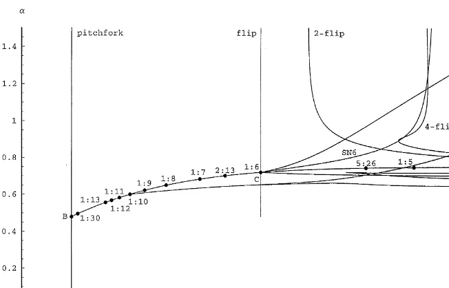
Fig. 1 shows a detailed bifurcation diagram on the (b,a)-plane (fora"10, p2"0.1, C"1, R"1.01, g"1.2)6 which we generated by the use of the LOCBIF program.
Fig. 1. Two parameter bifurcation diagram w.r.t.banda. 2-Hopf denotes a Hopf bifurcation curve for a 2-cycle, 2-#ip and 4-#ip denote#ip bifurcation curves of 2- and 4-cycles, respectively; SNn
denote saddle-node bifurcation curves of periodnpoints. The dots on the Hopf bifurcation curve de"ne origin points ofp:qArnold tongues. Note, thatB"(bH,aH) andC"(bF,aHH).
saddle-node bifurcation curves of periodqpoints, corresponding to a collision between stable and unstable periodic orbits of F (the map which de"nes the dynamical system (10)). In Fig. 1, a 1:10 Arnold tongue is drawn and origin points of some further Arnold tongues are plotted. Asbincreases,p/qincreases. B"(bH,aH) is the intersection point of the pitchfork bifurcation curve, the Hopf bifurcation curve (20), and the lineg(g!2)#2ap2a"0 (see Fig. 1). At Bthe pitchfork bifurcation changes from sub- to supercritical and expression (13), which determines the non-fundamental steady states, is not de"ned. When approachingBalong the Hopf bifurcation curve one eigenvalue of the Jacobian of the non-fundamental steady states converges to!1
2and the two complex
conjugate eigenvalues on the unit circle converge to 1, i.e. argj2,3"0 (for details see the appendix). A situation where a double eigenvalue 1 occurs would correspond to a 1:1 resonance (see for example Kuznetsov, 1995, Chapter 9.5.2). However, in our model B is a singularity on the (b,a)-plane, the dynamical system only consists of"xed points for a"aH. In the appendix we show that when approaching B from di!erent directions the eigenvalues have di!erent limits.
7In the class ofalldynamical systemsCwould be a point of codimension three. In our special family of systems, however, the 1:6 resonance follows from the simultaneous occurence of the Hopf and#ip bifurcations.
conjugate eigenvalues j2,3"A$Bi lying on the unit circle. Since j1"!j2j3/(j2#j3)"!(A2#B2)/2A(c.f. appendix, proof of Proposition 2), A"1
2 and B" J3
2, thus argj2,3"arctanJ3"2p16. Point C is the origin of
a 1:6 Arnold tongue.7
Between the pointsCandBany resonancep:qwith 0/1(p/q(1/6 can be found, which implies in particular all 1:q (q'6) resonances. p/q increases monotonically asbis increased. The computation of these points is described in the appendix.
For valuesa'aHHwe either havebF(b
H(a) orbH(a)NRand the secondary
bifurcation of the non-fundamental steady states is a#ip bifurcation. In Fig. 1, besides the Hopf bifurcation curve of the non-fundamental steady state de-scribed in Proposition 2, a Hopf bifurcation curve of the 2-cycle (which was created by the#ip bifurcation) starts in point C. Thus, for the chosen parameter values, the 2-cycle becomes unstable by a Hopf bifurcation which results in two attracting invariant cycles. After a saddle-node bifurcation of the sixth iterate of Fa stable (and an unstable) 6-cycle is created, lying in an Arnold tongue which originates inC. From the bifurcation diagram in Fig. 2(a) we conclude that this 6-cycle is destabilized by a period doubling bifurcation.
Let us now return to the general case of time varying beliefs on conditional variances of returns, i.e. wp,wk3(0, 1). The equilibria of the "ve-dimensional system (10) are the fundamental steady state E
1"(0,0,0,0,0) and the
non-fundamental steady states E
2"(xH,xH,xH, 0,( 1!R)xH) and E3"!E2, where
xHis given by (13), replacingp2byp2d.
Proposition3. In the case of timevarying beliefs about conditionalvariances of returns(0(w
p,wk(1)the primary bifurcation of the fundamental steady state and
the secondary bifurcations of the non-fundamental steady states are identical as in the case with constant beliefs aboutvariances(w
p"wk"1). Proof. See the appendix.
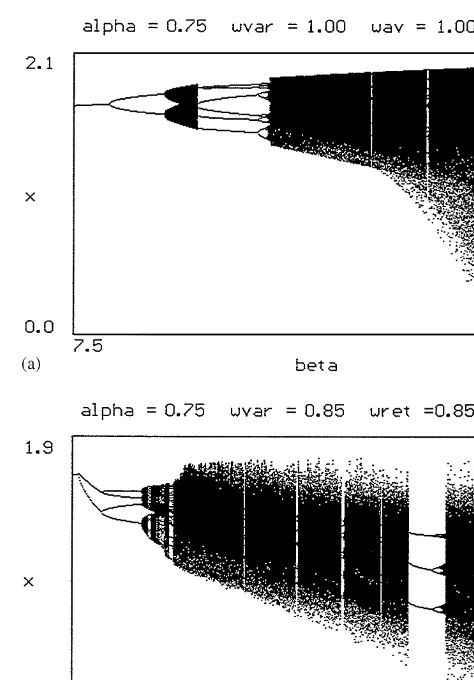
Fig. 2. Bifurcation diagrams plotting long-run behavior versus intensity of choicebfor (a) constant beliefs about conditional variances of returns, (b) time varying beliefs about conditional variances of returns (wvar"w
p, wret"wk).
Numerical simulations show that increasingbfurther leads to the occurrence of strange attractors. We will study the global dynamics and the occurrence of strange attractors in the next section.
4. Global dynamics
8The stable and unstable manifolds of a steady statex
0of a dynamical system corresponding to the mapFare de"ned as=s(x
0)"Mx: limn?=Fn(x)"x0Nand=u(x0)"Mx: limn?~=Fn(x)"x0N, resp., whereFndenotes thenth iterate ofF.
9For a brief introduction to the concept of homoclinic orbits see BH (1997a) and BH (1997b, 1998), Goeree and Hommes (1999) in this issue also recall this notion. An extensive mathematical treatment of homoclinic bifurcation theory can be found in Palis and Takens (1993).
10For the notion of a strange attractor see for example Palis and Takens (1993, Chapter 7.2). A mapFhas a horseshoe if there exist rectangular regionsRsuch thatFn(R) is folded overRin the form of a horseshoe, for somen3N.
varying variances) directions. If the unstable and the stable manifolds8intersect (in a so-called homoclinic point) this gives rise to very complicated behavior (as was already noticed by PoincareH at the end of last century). To understand the global dynamics of the system it is thus useful to study the geometric shapes of these manifolds. It will also give insight into the economic mechanism generat-ing complicated#uctuations.
In order to get insight into the dynamics we"rst consider the limiting case b"R. In this case the stable and unstable manifolds can be analyzed analyti-cally. In what follows we suppress the index 1 for the fundamental steady state E
1.
Proposition4. LetC'0andb"R.If
g'R and a' R2
2ap2dg2(2g!R2)
the unstable manifold of the fundamental steady stateEis bounded and all orbits converge to the saddle point E.
Proof. See the appendix.
11Note, that when the system is studied in the (x,y,z)-plane, (0,1,0) is a generalized eigenvector. For further analysis of the global geometric properties of the unstable mani-fold we restrict to the case with constant beliefs about variances (w
p"wk"1). Recall that the dynamical system is three dimensional in that case. We rewrite system (10) in the (x,y,m)-space, which yields
x
We will use the notation (x
t`1,yt`1,mt`1)"Fb(xt,yt,mt).
Next we consider the stable and unstable manifolds of the fundamental steady stateE. The stable manifold ofEis tangent to the planeS"Mx"0Nsince the stable eigenspace is spanned by the eigenvectors (0,1,0) and (0,0,1).11Forb"R the stable manifold ofEcontains the planeSsince every point inSis mapped onto E. In this case agents switch in"nitely fast between the predictors, the di!erence of the fractions is given by (22), resp. by
m
Any point lying on the planeMm"1Nis mapped onto the planeS. LetA
0be the
point on the unstable manifold where all agents switch from being trend chasers to fundamentalists, i.e. them-coordinate ofA
0is!1, but on the the right-hand
Fig. 3. Unstable manifold for case 1 (a"0.65,b"500):"rst 6 iterates of the segmentEA
0.
F3=(EA
0)"EA1XA@1A2XA@2A3,
F4=(EA
0)"EA1XA@1A2XA@2A3XA4,
F5=(EA
0)"EA1XA@1A2XA@2A3XA4XE.
F5=(EA
0) de"nes the unstable manifold forb"R. Our analysis implies that for
large but"nitebthe system must be close to having a homoclinic orbit between the stable and the unstable manifolds. But to see whether this implies complic-ated dynamics one needs compliccomplic-ated horseshoe constructions.
A numerical analysis of the unstable manifold for"niteb-values is presented in the appendix. We observe two cases. For su$ciently largea-values (case 2, see Fig. 7) the unstable segmentEA
0is expanded and folded over (close to) itself by
the 6th iterate of F
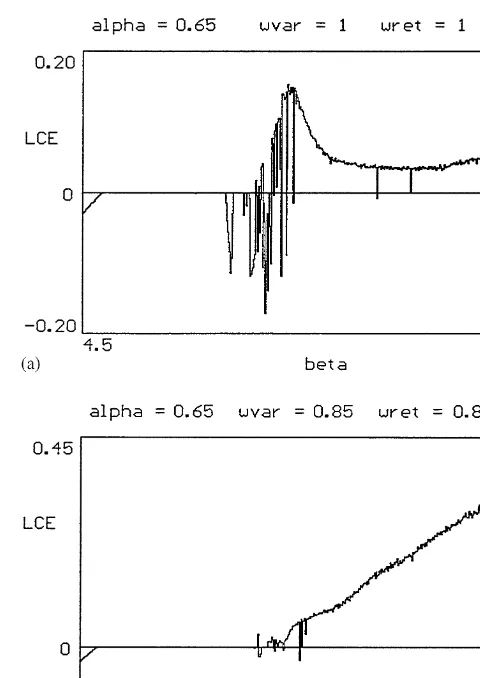
12BH (1998) brie#y explain the concept of Lyapunov exponents, see also the references there. Medio (1992, Chapter 6), also gives an introduction into that concept.
To show that chaos arises indeed we compute the largest Lyapunov character-istic exponents12(LCE) for the system. LCE measure the asymptotic exponential rate of divergence (resp. convergence) of two trajectories starting close to each other. Hence a positive LCE means that nearby trajectories separate exponenti-ally as time goes by and the system exhibits sensitive dependence on initial states and therefore chaos. Whenbbecomes su$ciently large we"nd positive LCE for both cases, 1 and 2, and also for the model with time varying beliefs about conditional variances. Thus, a high intensity of choice gives rise to chaotic dynamics. Fig. 4 shows the largest LCE for examples corresponding to case 1.
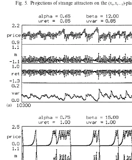
Figs. 5 and 6 show phase portraits in the (x
t,xt~1)-plane and time series of
strange attractors. We observe that the shape of the attractors may di!er for the cases with constant and time varying beliefs about variances as long as the intensity of choice is not too high. For largebthe projections of the attractors look very similar to the projection of the unstable manifold ofEon the (x
t,xt~1
)-plane (cf. Figs. 3 and 7) for all cases.
Our analysis also gives insight into the underlying economic mechanism. When prices are close to the fundamental both predictors give good forecasts. Since the fundamental predictor is costly most agents choose the trend chasing predictor which causes prices to move away from the fundamental value. At a certain point the stabilizing forceagives enough weight to the fundamentalists to push prices back to the fundamental. This leads to an irregular switching between periods where prices are close to and periods where prices are far above or below the fundamental. Fig. 6(a) shows a time series with such an irregular switching between periods where prices are close to the fundamental steady state, followed by an upward trend, after some unstable phase away from the fundamental value returning back and getting stuck near the locally unstable fundamental steady state and later moving away again. Fig. 6 also shows time series of returns. We observe periods with high and low volatilities.
For prices to return to the fundamental value the intensity of choice has to be high enough. In our numerical examples we observe that, in the case where the beliefs about variances vary over time, the intensity of choiceb has to be even larger, compared to the case with constant beliefs about variances (cf. Fig. 5). This stems from the fact that the same parameter values are used forp2andp2d, respectively. Therefore, the total variance in the case of time varying variances, p2
t#p2d, is larger and hence the performance;htis lower, which has a similar
e!ect as decreasingb.
Fig. 4. Largest Lyapunov characteristic exponents.
where prices lie below the fundamental value results in a dynamics which is symmetrical, with negative price deviations. However, adding some noise to system, as prices come close to the fundamental the market might switch between&optimistic'periods where prices are higher than the fundamental and &pessimistic'periods with prices#uctuating below the fundamental value.
5. Conclusions
Fig. 5. Projections of strange attractors on the (x
t,xt~1)-plane.
Fig. 6. Time series of price deviations from the fundamentalx
t, di!erences in the fractionsmt, and
Fig. 7. Unstable manifold for case 2 (a"0.75,b"2000): (a) the"rst 4 iterates of the segmentEA
0, (b) the 4th iterate and the beginning and end (dotted
line) of the 5th iterate ofA
0A@0A1.
A.
Gaunersdorfer
/
Journal
of
Economic
Dynamics
&
Control
24
(2000)
799
}
predictor based on fundamentals and a technical, trend chasing predictor. Choice of predictors is not only determined by their performance in the recent past but also by market conditions. Though the model is still very simple and stylized it possesses rich dynamics. As the intensity of choice to switch between predictors increases, di!erent bifurcation routes to chaotic price dynamics are possible. They depend (among other things) upon the strength of the stabilizing forcea. One could interpretaas a parameter that determines the probablility that traders do not choose the technical predictor when prices are too far away from the fundamental value, even when its recent performance was good. We have observed di!erent periods in the market where prices switch between stable phases close to the fundamental and unstable periods with prices much higher or much lower than the fundamental value.
Introducing the parameter a as a stabilizing force has allowed for a two parameter bifurcation analysis focusing on codimension one bifurcation curves. Such bifurcations generally occur in higher dimensional systems also. Though the way we introduced this stabilizing force here is rather&ad hoc'our analysis is useful. Similar codimension bifurcation routes may be expected in extensions of the model where the stabilizing force is modelled explicitely.
We further have introduced time varying beliefs about conditional variances of returns. The bifurcation routes to chaos di!er in some details, however the global qualitative features of the price dynamics are similar to the case with constant beliefs about variances. In real markets traders would not only update their expectations about future returns but use observed data also to estimate variables such as variances of returns. Our analysis gives a justi"cation to concentrate on the more tractable model with constant beliefs about variances, when trying to understand the behavior of"nancial markets.
The aim of the model is to understand stochastic properties of stock returns and trading volume observed in real"nancial data and the forces that account for these properties. Though statistical techniques are useful they are no substi-tute for a structural model in giving insight into the economic mechanism that may generate nonlinearity and observed#uctuations. Simple stylized versions of adaptive belief systems as presented in this paper also complement computer experiments like that of Arthur et al. (1997a, b) since they are able to analyze certain issues in an analytic framework. Such a scienti"c understanding is essential for a design of intelligent regulatory policy and also has practical value concerning risk management.
We have observed that the model generates time series of returns with periods of high and low volatilities. Though the time series of the actual model do not possess GARCH e!ects it seems promising that a further development of the model may generate such e!ects. Introducing more types may give price series with stochastic properties which are closer to real "nancial data. Also an improvement in the conditional rules for predictor choice which does not cause such an abrupt decline in prices as we have seen in some time series will be a step into this direction.
6. For further reading
Brock (1993).
Appendix
Proof of Proposition1. Steady statesx are given by
Rx"n
2gx"
1!mH 2 gx,
wheremHis the value ofm
tfor xt"xt~2"xH. It follows thatx"0 or
mH"1!2R
g"tanh
C
b 2A
g
2ap2xH(g xH!2xH)#axH2!C
BD
,i.e. xH2"2ap2(log (g/R!1)#bC)
b(g(g!2)#2ap2a) . (13)
Thus, besides the fundamental steady state E
1there exist two non-fundamental
equilibria E
2,3"($xH,$xH,$xH) i!
log(g/R!1)#bC
g(g!2)#2ap2a'0 and g'R.
The Jacobian of the fundamental steady state E
1 has the eigenvalue j1"
(g/2R)(1#tanh(bC/2)), which lies in the interval (0,1) i! b(bH" (1/C) log[g/(g!R)], and a double eigenvaluej2"j
3"0.
Forg52R, j1'1 (in that caseaH'0 and thereforea'aH, and bH(0). In Fig. 1,aHandbHare the coordinates ofB. h
Proof of Proposition 2. The characteristic polynomial of the Jacobian of the
non-fundamental steady states E
2and E3is given by
p(j)"j3!
A
1#g!2ap2awhere
Z:" b
ap2(g!R)xH2"2(g!R)
log(g/R!1)#bC
g(g!2)#2ap2a. (15)
Note that a change inais locally equivalent to a change in the risk parameter anear all steady states.
At the pitchfork bifurcation value b"bH, xH"0 (Z"0) and p(j) has a double eigenvalue 0 and an eigenvalue 1. For b slightly larger than bH(Z slightly positive),p(j) has three real, one negative and two positive eigenvalues inside the unit circle and the non-fundamental steady states are stable.
Increas-ingb, one of the two positive eigenvalues increases, the other one decreases. For
a certain value ofbthey coincide resulting in a double real positive eigenvalue inside the unit circle, increasingb further, two complex conjugate eigenvalues occur. These eigenvalues might cross the unit circle at a valuebH(a), given by (19) and (20), respectively. In this case a Hopf bifurcation of the non-funda-mental steady states occurs.
Letj1,j2,j3denote the eigenvalues, wherej2,3"A$Bi. Sincep(j) has no linear term,j1"!j
2j3/(j2#j3). Therefore,
p(j)"(j!j1) (j2!(j2#j3)j#j2j3)
"
A
j#A2#B22A
B
(j2!2Aj#A2#B2)"j3#
A
A2#B22A !2A
B
j2#(A2#B2)2
2A . (16)
Hopf bifurcation of the non-fundamental steady states: A Hopf bifurcation of the non-fundamental steady states occurs ifA2#B2"1. By comparing coe$cients of (14) and (16) this yields
1#g!2ap2a
g Z"!
1
2A#2A and (g!1)Z"
1
2A. (18)
EliminatingAfrom these equations, we obtain that on the (b,a)-plane the Hopf bifurcation curve is implicitely de"ned by
(g2!2ap2a)(g!1)
g Z2#(g!1)Z!1"0. (19)
Using (15), (19) can be rewritten as
4(g2!2ap2a)(g!1)(g!R)2
A
logA
gR!1
B
#bCB
2
#2g(g!1)(g!R)(g(g!2)#2ap2a)
A
logA
gR!1
B
#bCB
From (19) we further have
Z"!g(g!1)$Jg2(g!1)2#4g(g!1)(g2!2ap2a) 2(g2!2ap2a)(g!1) ,
which is real for
a( 1
8ap2g(5g!1)":a6.
On the (b,a)-plane the Hopf bifurcation curvea(b) obtains its maximum at a6 (cf. Fig. 1).
Flip bifurcation of the non-fundamental steady states: A#ip bifurcation of the non-fundamental steady states occurs for j1"!(A2#B2)/2A"!1. Com-paring coe$cients of (14) and (16) gives
1#g!2ap2a
g Z"!1#2A and (g!1)Z"A2#B2.
EliminatingAandB, we obtain
Z" 2g
g(g!2)#2ap2a
and plugging this expression into (15) yields
b"bF"1
C
A
g
g!R!log
A
g R!1
BB
.PluggingbFinto (20) we obtain two solutions fora,
a1"!g(5g!6)
2ap2 (aH Q g'1,
a2" g2
2ap2"aHH(a6 Q g'1.
Sinceg'R('1) (otherwise non-fundamental steady states do not exist), the #ip bifurcation lineb"b
Fintersects the Hopf bifurcation curve inC"(bF,aHH)
(see Fig. 1, recall that B"(bH,aH)). Therefore, if a3(aH,aHH) the non-funda-mental steady states are destabilized by a Hopf bifurcation atb"b
H(a) de"ned
by (20),bH(a)(b
Fin that case. Ifa3(aHH,a6], bF(bH(a), ifa'a6, bH(a)NR, thus
A.1. Limits of the eigenvalues when approachingB
On the Hopf bifurcation curve (19), asaPaH,g2!2ap2aP2g(g!1), there-fore fora+aH(19) can approximately be written as
2(g!1)2Z2#(g!1)Z!1"0,
hence lim
(b,a)?BZ"1/(2(g!1)) along the Hopf bifurcation curve. Thus, in the
limit (14) reduces to
j3!3
2j2#12"0,
which has zeros 1 (double) and!1 2.
Approaching point B along the Hopf bifurcation curve the two complex conjugate eigenvalues on the unit circle therefore converge to 1 and the third eigenvalue to!1
2.
On the pitchfork bifurcation line the fundamental and the non-fundamental steady states coincide. The eigenvalues of the steady state are 0 (double) and 1. On the line g(g!2)#2ap2a"0 (on the (b,a)-plane this is a horizontal line through point B"(bH,aH), see Fig. 1) the characteristic Eq. (14) reduces to a quadratic equation with zeros $1. As a approaches aH (from above) one eigenvalue tends to in"nity.
A.2. Computations of the origin points of Arnold tongues
On the Hopf bifurcation curveA2#B2"1, using (18) we have
argj"arctanB
A"arctan
J1!A2
A
"arctan
C
2g(g!1)ZS
1! 14(g!1)2Z2
D
.Hence plugging expression (15) in forZwe obtain
tan
A
2pp qB
"J16(g!1)2(g!R)2(log(g/R!1)#bC)2!(g(g!2)#2ap2a)2
g(g!2)#2ap2a ,
resp.
16(g!1)2(g!R)2
A
logA
gR!1
B
#bCB
2
!(g(g!2)#2ap2a)2
"(g(g!2)#2ap2a)tan2
A
2ppFor anyp/qwe obtain the origin points of the Arnold tongues on the (a,b)-plane, as the solutions of (20) and (21). Note that four angles argjgive the same value for tan2(argj). From the second equation of (18) we conclude that the eigen-values corresponding to the Hopf bifurcation curve have non-negative real part (when moving away from B along the Hopf bifurcation curve (20) the two complex conjugate eigenvalues move on the unit circle from #1 to $i as bPR). Therefore,pandqhave to be chosen such that 2p(p/q)3[0,p/2] (p/q reduced) to get a p:q resonance. From (18) it also follows thatp/qincreases monotonically whenbis increased.
Proof of Proposition 3. It is easy to check that the eigenvalues of the funda-mental steady state E
1are (g/2R)(1#tanh (bC/2)) and 0(2)(which are the same
as in the case of constant beliefs about variances) and the two stable eigenvalues w
pThe characteristic polynomial of the Jacobian,wk3(0, 1). J of the non-fundamental steady states is given by
det (J!jI)"(w
p!j)(wk!j) det (J#!jI),
whereJ
#is the Jacobian for the case with constant beliefs about variances when
p2is replaced byp2d. Therefore, in addition to the stable eigenvalueswpandwk, we have the same eigenvalues as in the case of constant beliefs about vari-ances. h
Proof of Proposition4. We proceed analogous as in the proof of Lemma 4 in BH
(1998). We have
The unstable eigenvector of the fundamental steady state is
13The numerical computations of the unstable manifolds were carried out by plotting 6000 equally spaced points on a small unstable eigenvector according to thej-lemma (see Guckenheimer and Holmes, 1986, p. 247). (To get accurate pictures, we further iterated segmentA
1A@1and some small subsegments onA
1A@1taking even more, namely, 30,000 points.) Take an initial state x
is positive there is some smallest ¹'0 such that C
T'C, so that
m
T"#1,xt"0∀t5¹#1, and mt"!1 ∀t5¹#3. Hence in this case
the unstable manifold is bounded and all orbits converge toE. h
A.3. Numerical analysis of the unstable manifold of the fundamental steady stateEfor large butxniteb
Numerical computations suggest that the situation is similar as in BH (1997a) and in Goeree and Hommes (1999). However, our system is three dimensional, therefore the analysis of the unstable manifold ofEfor large but"nitebis much more delicate than for the two-dimensional models in those papers. An approxi-mation of the unstable manifold is not obtained by connecting the segments of F5=(EA
0) just by straight segments. The limiting manifold will contain line
segments lying on the planesMm"!1NandMm"1Nwhich are connected by vertical line segments. Of course,A
1and A@1are connected by a vertical line
segment. Note that forb"R,m
tin (11) is not de"ned if equality holds on the
right-hand side of (12). We have de"ned m
t"!1 in that case, however, we
could have taken any other value between!1 and 1. One could interpret the vertical line segement A
1A@1 as image of A0. For "nite but su$ciently large
b there is a segmentA
0A@03EA1whose image is close to the vertical segment
A
1A@1. Further analysis will be carried out numerically.
We"nd that, depending ona, two cases are possible. Figs. 3 and 7 show the "rst six resp. "ve iterates of the unstable manifold for g"1.2, R"1.01,a"10, p2"0.1,C"1.13 We analyze case 1 for the numerical examplea"0.65, case 2 fora"0.75.
Case 1: For b su$ciently large the unstable manifold is arbitrary close to (see Fig. 3)
F(EA0)"EA1,
F2(EA
F3(EA
i (the points which de"ne the segments of the unstable
manifold in the caseb"R),X@denotes points lying on the planeMm"!1N having the samexandy-coordinates asX3Mm"1N.Fdenotes the limit ofF
b asbPR.
Case 2: Fig. 7(a) shows EA
0A@0 and the "rst three iterates of the segment
A
0A@0A1 ("rst four iterates of EA0), Fig. 7(b) shows the fourth iterate of the
segmentA
0A@0A1and the"rst and last part (dotted line) of its"fth iterate. The
"rst three iterates ofEA
0are as in case 1. For further iterations we obtain
F4(EA
For the 6th iterate we only roughly sketch the approximative way of the unstable manifold:
0) denotes the reverse direction of F4(EA0). When moving between the
points (close to)A
2andA@23Mm"1Nparts of the connecting segment lie in the
planeMm"!1N, similar as forF4(EA
0) andF5(EA0). Though this description
is rather rough it shows that the 6th iterate ofEA
0contains segments which are
expanded and folded along (close to) the unstable segmentEA
0. This suggests
that for su$ciently largeb-values,F6bhas as a full horseshoe over a rectangular region containing a subsegment ofEA
0.
Note that in both cases the unstable manifold gets arbitrarily close to the planeSwhich is contained in the stable manifold. That is, the unstable manifold "rst moves away from the fundamental steady state but returns close to it later on (cf. Proposition 4).
Case 1 appears to be similar to the case of Fig. 8(e}f) in Goeree and Hommes (1999). The fourth iterate ofEA
0does not contain the segmentC7C@7C@8C8as in
case 2. Indeed, whenais decreased,C
7andC8approach each other turning case
2 into case 1 for a certain value of a. It is not clear whether a horseshoe construction as in case 2 is possible. Numerically, all points of the segment A
1A@1A2 are mapped to the steady state E after four iterates. The 6th iterate
might continue to move alongEA
0. Computing LCE shows that chaos arises in
that case also (see Section 4).
References
Allen, F., Gorton, G., 1993. Churning bubbles. Review of Economic Studies 60, 813}836. Anderson, S., de Palma, A., Thisse, J., 1993. Discrete Choice Theory of Product Di!erentiation. MIT
Press, Cambridge, MA.
Arrowsmith, D.K., Place, C.M., 1990. An Introduction to Dynamical Systems. Cambridge Univer-sity Press, Cambridge, UK.
Arthur, W.B., Holland, J.H., LeBaron, B., Palmer, R., Tayler, P., 1997a. Asset pricing under endogenous expectations in an arti"cial stock market. In: Arthur, W.B., Durlauf, S.N., Lane, D.A. (Eds.), The Economy as an Evolving Complex System II. Addison-Wesley, Reading, MA, pp. 15}44.
Arthur, W.B., LeBaron, B., Palmer, R., 1997b. Time series properties of an arti"cial stock market. University of Wisconsin, SSRI working paper 9725.
Barucci, E., Posch, M., 1996. The rise of complex beliefs dynamics. IIASA working paper WP-96-46. Beja, A., Goldman, B., 1980. On the dynamic behavior of prices in disequilibrium. Journal of
Finance 35, 235}248.
Black, F., 1986. Noise. Journal of Finance 41, 529}543.
Blume, L., Easley, D., 1992. Evolution and market behavior. Journal of Economic Theory 58, 9}40.
Bollerslev, T., Engle, R.F., Nelson, D.B., 1994. ARCH models, In: Engle, R.F., McFadden, D.L. (Eds.), Handbook of Econometrics. Elsevier, Amsterdam, pp. 2959}3038.
Brock, W.A., 1993. Pathways to randomness in the economy: emergent nonlinearity and chaos in economics and"nance. Estudios EconoHmicos 8, 3}55.
Brock, W.A., 1997. Asset price behavior in complex environments. In: Arthur, W.B., Durlauf, S.N., Lane, D.A. (Eds.), The Economy as an Evolving Complex System II. Addison-Wesley, Reading, MA, pp. 385}423.
Brock, W.A., Hommes, C.H., 1997a. A rational route to randomness. Econometrica 65, 1059}1095. Brock, W.A., Hommes, C.H., 1997b. Models of complexity in economics and"nance. In: Heij, C., Schumacher, H., Hanzon, B., Praagman, K. (Eds.), System Dynamics in Economic and Financial Models. Wiley, Chichester, pp. 3}44.
Brock, W.A., Hommes, C.H., 1998. Heterogeneous beliefs and bifurcation routes to chaos in a simple asset pricing model. Journal of Economic Dynamics and Control 22, 1235}1274.
Brock, W.A., Hsieh, D.A., LeBaron, B., 1991. Nonlinear Dynamics, Chaos, and Instability. MIT Press, Cambridge, MA.
Brock, W.A., Lakonishok, J., LeBaron, B., 1992. Simple trading rules and the stochastic properties of stock returns. Journal of Finance 47, 1731}1764.
Brunnermeier, M.K., 1998. Prices, price processes, volume and their information*A survey of the market microstructure literature. FMG discussion paper 270, The London School of Economics. Chiarella, C., 1992. The dynamics of speculative behaviour. Annals of Operations Research 37,
101}123.
Day, R.H., Huang, W., 1990. Bulls, bears and market sheep. Journal of Economic Behavior and Organization 14, 299}329.
De Grauwe, P., Dewachter, H., Embrechts, M., 1993. Exchange Rate Theory. Blackwell, Oxford. De Long, J.B., Shleifer, A., Summers, L.H., Waldmann, R.J., 1990a. Noise trader risk in"nancial
markets. Journal of Political Economy 98, 703}738.
De Long, J.B., Shleifer, A., Summers, L.H., Waldmann, R.J., 1990b. Positive feedback investment strategies and destabilizing rational speculation. Journal of Finance 45, 379}395.
Franke, R., Sethi, R., 1993. Cautious Trend-Seeking and Complex Dynamics. University of Bielefeld. Frankel, J.A., Froot, K.A., 1988. Chartists, fundamentalists and the demad for dollars. Greek
Economic Review 10, 49}102.
Genc7ay, R., Stengos, T., 1997. Technical trading rules and the size of the risk premium in security returns. Studies in Nonlinear Dynamics and Econometrics 2, 23}34.
Ghezzi, L.L., 1992. Bifurcations in a stock market model. Systems & Control Letters 19, 371}378. Goeree, J.K., Hommes, C.H., 1999. Heterogeneous beliefs and the nonlinear cobweb model. Journal
of Economic Dynamics and Control, this issue.
Grandmont, J.-M., 1998. Expectations formations and stability of large socioeconomic systems. Econometrica 66, 741}781.
Grossman, S.J., 1989. The Informational Role of Prices. MIT Press, Cambridge, MA.
Guckenheimer, J., Holmes, P., 1986. Nonlinear Oscillations, Dynamical Systems, and Bifurcation of Vector Fields. Springer, New York.
Haugen, R.A., 1998a. Beast on Wall Street*How Stock Volatility Devours Our Wealth. Prentice-Hall, Englewood Cli!s, NJ.
Haugen, R.A., 1998b. The Ine$cient Market*What Pays O!and Why. Prentice-Hall, Englewood Cli!s, NJ.
Haugen, R.A., 1998c. The New Finance*The Case for an Over-reactive Stock Market. Prentice-Hall, Englewood Cli!s, NJ.
Hommes, C.H., Sorger, G., 1998. Consistent expectations equilibria. Macroeconomic Dynamics 2, 287}321.
Khibik, A.H., Kuznetsov, Y.A., Levin, V.V., Nikolaev, E.V., 1992. LOCBIF. An interactive LOCal BIFurcation analyzer.
Kurz, M. (Ed.), 1997. Endogenous Economic Fluctuations. Springer, Berlin.
Kuznetsov, Y.A., 1995. Elements of Applied Bifurcation Theory. Springer, New York.
LeBaron, B., 1995. Experiments in Evolutionary Finance. Department of Economics, University of Wisconsin.
Lux, T., 1994. Complex dynamics in speculative markets: a survey of the evidence and some implications for theoretical analysis. Volkswirtschaftliche DiskussionsbeitraKge 67, University of Bamberg.
Lux, T., 1995. Herd behavior, bubbles and crashes.. The Economic Journal 105, 881}896. Lux, T., Marchesi, M., 1998. Volatility in"nancial markets: a micro-simulation of interactive agents.
Working paper presented at the Third Workshop on Economics with Heterogeneous Interacting Agents, University of Ancona.
Medio, A., 1992. Chaotic Dynamics: Theory and Applications to Economics. Cambridge University Press, Cambridge, UK.
Nelson, D.B., 1992. Filtering and forecasting with misspeci"ed ARCH Models I: getting the right variance with the wrong model. Journal of Econometrics 52, 61}90.
Sargent, T.J., 1993. Bounded Rationality in Macroeconomics. Clarendon Press, Oxford. Sethi, R., 1996. Endogenous regime switching in speculative markets. Structural Change and
Economic Dynamics 7, 99}118.
Shiller, R.J., 1991. Market Volatility. MIT Press, Cambridge, MA.
Shleifer, A., Summers, L.H., 1990. The noise trader approach to "nance. Journal of Economic Perspectives 4, 19}33.
Smale, S., 1965. Di!eomorphisms with many periodic points. In: Cairns, S.S. (Ed.), Di!erential and Combinatorical Topology. Princeton University Press, Princeton, NJ, pp. 63}80.
Thaler, R.H., 1991. Quasi Rational Economics. Russel Sage Foundation, New York.
Thaler, R.H. (Ed.), 1993. Advances in Behavioral Finance. Russel Sage Foundation, New York. Viana, M., 1993. Strange attractors in higher dimensions. Boletim da Sociedade Brasileira de