24 (2000) 1007}1026
Adaptive learning of rational expectations
using neural networks
Maik Heinemann
*
University of Hannover, Institute of Economics, Ko(nigsworther Platz 1, D-30167 Hannover, Germany
Abstract
This paper investigates how adaptive learning of rational expectations may be modeled with the help of neural networks. Necessary conditions for the convergence of the learning process towards (approximate) rational expectations are derived using a simple nonlinear cobweb model. The results obtained are similar to results obtained within the framework of linear models using recursive least squares learning procedures. In general, however, convergence of a learning process based on a neural network may imply that the resulting expectations are not even local minimizers of the mean-squared
prediction error. ( 2000 Elsevier Science B.V. All rights reserved.
JEL classixcation: C 45; D 83
Keywords: Adaptive learning; Neural networks; Rational expectations
1. Introduction
Dynamic economic models usually require that agents within the model form expectations regarding future values of economic variables. Assumptions about how the agents form their expectations may then have far reaching conse-quences for conclusions derived from a particular model. The hypothesis of
rational expectations states that the agents'knowledge of their economic
envi-ronment is such that the objective distributions of the relevant variables are
*Tel.: 49-511-762-5645; fax: 49-511-762-5665.
E-mail address:[email protected] (M. Heinemann)
known to them. Thus, their expectations are based upon this objective distribu-tions. In this extreme form, the hypothesis of rational expectations is naturally
subject to criticism. As Sargent (1993, p. 3) remarks:&[2] rational expectations
models impute much more knowledge to the agents within the model [2] than is
possessed by an econometrician, who faces estimation and inference problems that agents in the model have somehow solved'. Hence the question is, whether it is possible to establish rational expectations as a result of learning processes, without imposing such strong assumptions regarding the knowledge of the agents within the model.
One possible approach is to assume that the agents do not have any prior knowledge about the objective distributions of relevant variables, but instead are equipped with an auxiliary model describing the perceived relationship between these variables. In this case, agents are in a similar situation as the econometrician in the above quotation: They have to estimate the unknown parameters of their auxiliary model in order to form the relevant expectations on the basis of this model. This is but one possible notion of bounded rationality that is discussed in the economics literature. There exist many other approaches that try to capture the idea of limited knowledge and limited information processing capabilities of economic agents (cf. Conlisk, 1996). Nevertheless, in
this paper I will refer to the above-described framework as the &boundedly
rational learning approach'.
In the boundedly rational learning framework, the auxiliary model of the agents is correctly speci"ed at best in the sense, that it correctly depicts the
relationship between the relevant variables within the rational expectations
equilibrium, but the model is misspeci"ed during the learning process. While this implies that there may exist values for the parameters that result in rational expectations, the estimation problem faced by the agents is quite di!erent from usual estimation problems, because the expectations of the agents itself a!ect the
data underlying the estimation of parameters (&forecast feedback'). This means
that during the learning process the relationship between the variables observed by the agents, will change as long as the agents change their expectations scheme. The question, whether or not the estimated parameters will converge toward parameter values implying rational expectations is thus not a trivial one, because usual approaches to prove consistency of estimators are not applicable. In case of linear models, i.e. models where the rational expectations equilib-rium is a linear function of exogenous and lagged endogenous variables, recur-sive least squares can be used to estimate the parameters of the auxiliary model. Regarding this case, there are a number of contributions, where conditions for the converge of the learning process towards rational expectations are derived (cf. Bray, 1983; Bray and Savin, 1986; Fourgeaud et al., 1986; Marcet and Sargent, 1989).
variables, the analysis of adaptive learning procedures is more complicated. The problem is that the boundedly rational learning approach requires assumptions regarding the auxiliary model of the agents. It is obvious that the assumption of a correctly speci"ed auxiliary model is a very strong one, because such an assumption presupposes extraordinary a priori knowledge of the agents
regard-ing their economic environment.1But the removal of this assumption requires
that the auxiliary model of the agents is #exible enough to represent various
kinds of possible relationships between the relevant variables.
One way to achieve this#exibility is to assume that the auxiliary model of the
agents is a neural network. Neural networks might be well suited for this task because they are, as will be shown below, able to approximate a wide class of
functions at any desired degree of accuracy.2Thus, if the auxiliary model of the
agents is given by a neural network, they may possibly be able to learn the formation of rational expectations, without the requirement of knowledge regarding the speci"c relationship of the relevant variables.
However, the present paper demonstrates that such a con"dence in the power of neural networks might be too optimistic: First, if the agents in the model learn by estimating parameters of an auxiliary model, feedback problems will arise that might prevent the convergence of the learning process. As is shown below, it depends on the nature of the true model, i.e. upon how expectations a!ect actual outcomes, whether convergence and thus learning of rational expectations can occur. Second, there are still speci"cation problems present, because the prin-ciple ability of neural networks to approximate a wide class of functions does not mean that a concrete speci"ed network at hand is able to do so. A neural network that is misspeci"ed in this respect will clearly not enable the agents to learn rational expectations. The best one can hope for is that convergence towards approximate rational expectations occurs, i.e. expectations that are merely local minimizers of the mean squared prediction error. The paper shows, that the convergence to such approximate rational expectations cannot be ruled out even if the neural network is correctly speci"ed. Moreover, in general nonlinear models, neural network learning may result in expectations, that are not even local minimizers of the mean-squared prediction error.
At this point it is worth to be emphasized that neural networks represent but one among many other procedures that can be used to approximate an un-known function. Nevertheless, neural networks have gained much popularity recently, especially in econometrics, and are sometimes treated as if they do not face any speci"cation problems themselves. It should be noted, however, that
1A similar argument can be found in Salmon (1995).
many of the results that are derived below carry over to other approximation procedures as well.
In the following, a model is formulated, where agents have to form expecta-tions and use a neural network as their auxiliary model. In the next section, a simple reduced form equation will be speci"ed, where the value taken by an endogenous variable depends on its expected value and the values taken by exogenous variables. After that, the neural network used as auxiliary model of the agents in the model will be described. Then the learning algorithm will be formulated and the question will be investigated, whether or not the agents are able to form (approximate) rational expectations using neural net-works. Finally, a more general reduced form is considered in order to show that some of the results are due to the very special structure of the model analyzed so far.3
2. The model
2.1. A reduced form equation for the endogenousvariable
Consider a model, where agents have to form expectations regarding an endogenous variable, whose value depends on observable exogenous variables
and an unobservable error. The reduced form is given by4
p
t"ap%t#g(xt)#et. (1)
Herep%t denotes the agents'expectation of the endogenous variablepin period
tandp
tdenotes the actual value the endogenous variable takes in periodt.xtis
ak-dimensional vector of exogenous variables, which can be observed before the
expectationp%
t is formed. It is assumed thatxtis for allta vector of independent
and identically distributed random variables. Additionally it is assumed that
x
t is bounded for allt, i.e.xt takes only values in a set XxLRk. et is, like the
elements of x
t, for all t an independent and identically distributed random
variable that satis"es E[e
t]"0, E[e2t]"p2e and E[etDxt]"0. Like xt, et is
bounded for alltand takes values in a sete
t3XeLR. Contrary to the elements
of x
t, et is not observable by the agents, such that expectations regarding the
3The work of Salmon (1995) and Kelly and Shorish (1994) deals at least partially with a similar question like this paper. Both papers take neural networks as the basis of learning processes. While the conclusions of Salmon (1995) exclusively rely upon simulation results, Kelly and Shorish (1994) use a learning rule, which makes their results not comparable to those obtained here.
4Eq. (1) may be interpreted as the reduced form of a cobweb model if the endogenous variable pdenotes the price of the relevant good: Given the supply functiony4(p%t)"ap%tand the demand functiony$(p
endogenous variable cannot be conditioned on this variable. Finally, the
func-tiong(x) is a continuous function for allx3X
x.5
Reduced form (1) may be viewed as a special case of a more general class of
nonlinear models, where the value of the endogenous variablepin periodtis
given by p
t"G(z%t,yt,et). Herez%t is a vector of expectations regarding future
values of the endogenous variable,y
tis a vector of variables predetermined in
period t, e
t is an unobservable error andGmay be any continuous function.
Note thaty
tmay contain exogenous as well as lagged endogenous variables. As
shown by Kuan and White (1994a), the methodology used here to analyze learning processes based on the reduced form (1), can also be used to analyze this more general case. But contrary to the simple model (1), the required restrictions are quite abstract and it is not possible to derive conditions for convergence, which may be interpreted from an economic viewpoint. A more general reduced form than (1) will be considered below.
Given the reduced form (1) and because E[e
tDxt]"0, rational expectations are given by:
As long asaO1, there exists a unique rational expectation ofp
twhatever value
is taken by the exogenous variablesx
t. In what follows,/(xt) denotes the rational expectations function that gives this unique rational expectation of the
endogen-ous variable for allx3X
x.
It is obvious that the agents may not be able to form rational expectations if they do not know the reduced form of the model and especially the form of the functiong(x
t). The question is, whether the agents can learn to form rational
expectations, using observations of the variables p
t~1,pt~2,2 and x
t~1,xt~2,2. This means that the agents are at least aware of the relevant
variables that determine the endogenous variablep
tin a rational expectations
equilibrium. It is assumed that the agents have an auxiliary model at their disposal representing the relationship between the exogenous variables and the endogenous variable.
If g(x
t) is linear in xt, reduced form (1) becomes the linear model
p
t"ap%t#b@xt#et, wherebis ak-dimensional vector of parameters. This is the linear case mentioned in the introduction. Assuming that agents use the
auxili-ary modelp"d@x to represent the relationship betweenxandpand that the
parametersdare estimated using recursive least squares, the following can be shown (Bray and Savin, 1986; Marcet and Sargent, 1989):
(a) If the estimatordK for dconverges, this results in rational expectations, i.e.
dK"(1!a)~1b@.
(b) The estimator fordwill converge towards (1!a)~1b@if and only ifa(1.
As the function g(x
t) from (1) does not need to be linear in xt, the rational
expectations function/(x
t) needs not to be a linear function too. Thus, if one
assumes that agents use parametrically speci"ed auxiliary models and have no
prior knowledge regarding the functional form of/(x
t), it would be advisable to
take an auxiliary model that is#exible enough to approximate various possible
functional forms at least su$ciently well. The next subsection establishes that neural networks may be auxiliary models having the desired property.
2.2. Hidden layer neural networks
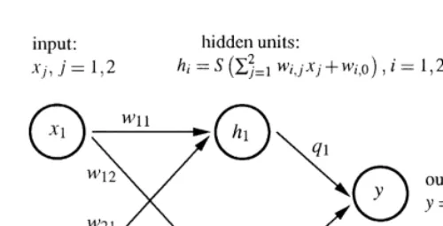
In the following a special form of neural networks is considered. These networks are called hidden layer neural networks and a typical structure is depicted in Fig. 1. In this type of networks, information proceeds only in one direction and there exists only one layer of hidden units between the input units and the output units.
Each of the hidden unitsi"1,2,mreceives a signal that is the weighted sum
of all inputsx
j, j"1,2,k. This implies thathIi"+jk/1wi,0#wi,jxjis the signal
received by the hidden uniti, wherew
i,0fori"1,2,mrepresents a threshhold value. In each hidden unit the signal received is transformed by an activation
functionS, such thath
i"S(hIi) is the output signal of the hidden uniti. Finally, the output unit receives the weighted sum of all these output signals, such that
y"+m
i/1hi#q0 is the output of the neural network, where q0 represents
a threshhold value. The so-de"ned mapping from inputsx
jto the outputygiven
by the so-speci"ed network may be written as follows:
y"q
network containskinput units andmhidden units,his aq-dimensional vector,
whereq"1#m(k#2).
A usual choice for the activation function is a continuous, monotone function, mapping the real numbers into the interval [0,1]. A function that exhibits this properties is
S(z)" 1
Fig. 1. A neural network with two input units, one output unit and one hidden layer consisting of two units.
What makes this kind of neural networks interesting with respect to the problem
of learning is their ability to approximate nearly any function.6
¹heorem2.1 (Hornik et al., 1989, Theorem 2.4). The neural network(3)with one layer of hidden units and activation functions given by(4)is able to approximate any continuous function dexned over some compact set to any desired accuracy if the network contains a suzcient number of hidden units.
Theorem 2.1 guarantees the existence of a neural network such that a suitably speci"ed distance between a given continuous function and this network
be-comes arbitrarily small. Thus, in what follows &perfect approximation' means
that we have such a neural network and a vector of parameters hHsuch that
/(x
t)"f(xt,hH) almost surely. Unfortunately, the theorem makes no statement
regarding the number of hidden units required in order to obtain such a perfect
approximation. This means that given a neural network (3) withmhidden units,
it is by no means guaranteed that a perfect approximation of the rational
expectations function /(x
t) is possible, i.e. the misspeci"cation of a neural
network cannot be ruled out a priori.
2.3. The objectives of learning
If it is assumed that the auxiliary model used by the agents in the model is
a neural network of form (3), the expectation ofpgiven a vector of parameters
h and observations x of the exogenous variables is given by p%"f(x,h). In general, this expectation turns out to be incorrect and the agents may wish to change the values of the parameters in order to enhance the predictive power of their model. This is what we call learning. Before this learning process is analyzed in more detail, it useful to be more precise regarding the objectives of learning.
It seems plausible to use the mean-squared error of the expectations as a measure for the success of learning. This mean-squared error is de"ned as the
expected value of the squared deviation of the agents' expectation about the
endogenous variable p%"f(x,h) from its actual value, which is given by
p"af(x,h)#g(x)#e.7Denoting this mean-squared error asj(h) we get
A plausible learning objective is to search for a vector hthat minimizesj(h).
Such an optimal vector of parametershHsatis"es
hH"argmin h|Rq
j(h) (6)
and the necessary condition for the associated optimization problem is given by
£
hj(h)"!2(1!a)2E
G
£hf(x,h)C
/(x)# e1!a!f(x,h)
DH
"0. (7)Note that the solution of (7) does not need to be unique. If there exists a vector of
parameters satisfying the condition£
hj(h)"0, it results in a (local) minimum of the mean-squared error if the Jacobian matrix
J is positive semide"nite. A (local) minimum athHis (locally) identi"ed ifJ
j(hH) is
positive de"nite. Otherwise, at least one eigenvalue of J
j(hH) equals zero, such that the minimum is not (locally) identi"ed. This means that there exists
a neighborhood of hH with vectors h that imply an identical value for the
mean-squared errorj(hH).
Now de"ne the set
HL"Mh3RqD£
hj(h)"0,Jj(h) is positive semide"niteN,
i.e.HLis the set of all vectors of parameters for the neural network implying
a}possibly not identi"ed}(local) minimum of the mean-squared errorj(h).
If the neural network is able to give a perfect approximation of the unknown
rational expectations function/(x), there exist vectors of parameters implying
j(h)"p2e. Note that in the neural network speci"ed here, all hidden units use identical activation functions, such that there will be no unique vector having this property. LetHG"Mh3RqD j(h)"p2eNdenote the set of all these vectors of
parameters. Obviously,HGis a subset ofHL.HGwill be empty if the number of
hidden units in the neural network is not su$cient to give a perfect approxima-tion of/(x).
Anyh3HG implies that the expectations formed on the basis of the neural
network coincide with rational expectations according to (2). This is not true for
the remaining vectors of parametersh3HLCHG: All these vectors of parameters
result in (local) minima of the mean squared errorj(h), but they do not imply
/(x)"f(h,x) almost surely. These vectors of parameters merely result in more or less accurate approximations of the unknown rational expectations function. Thus, following Sargent (1993), the resulting equilibria will be labeled as
approx-imate rational expectations equilibria.8
3. Learning of(approximate)rational expectations
As mentioned above, learning in the model considered here means that agents estimate the parameters of their auxiliary model on the basis of observations of exogenous and endogenous variables. The question, whether the agents are able to learn to form rational expectations is thus equivalent to the question, whether their estimation procedure yields asymptotically correct parameter values. This
is in turn equivalent to estimated parameter vectors that converge to ah3HG. If
the neural network used by the agents is not able to give a perfect
approxima-tion of the unknown funcapproxima-tion/(x), the question is, whether there will at least
result approximate rational expectations, i.e. whether the estimated parameter
vectors converge to ah3HL.
Given a vector of parametersh
t, the expectation function in periodtis given
asp%
t"f(xt,ht). Thus, from reduced form (1) the actual value of the endogenous
variable intis obtained as
p
t"af(xt,ht)#g(xt)#et.
8Properly speaking, as noted by Kuan and White (1994a), the label&incorrect belief equilibria'
Iff(x
t,ht)O/(xt), the agents'expectation turns out to be incorrect and the value
taken by the endogenous variable in t diverges from its value in the rational
expectations equilibrium.
In what follows it is assumed that the learning algorithm used by the agents is
the so called&backpropagation algorithm', a widely used algorithm in the neural
network literature.9This algorithm modi"es the vector of parametersh
t
accord-ing to the product of the actual expectational errorp
t!p%t"pt!f(xt,ht) and
the gradient of the neural network with respect toh
t: h
t`1"ht#ct`1[£hf(xt,ht)(pt!f(xt,ht)]. (9) Herectis a learning rate that satis"esct"t~i, 0(i41. The declining learning
rate implies that the modi"cations ofht according to (9) become smaller over
time. This is required in order to derive conclusions regarding the convergence of the vector of parameters.
The question, whether agents will asymptotically learn to form (approximate)
rational expectations is now equivalent to the question, whetherh
taccording to
(9) will converge to ah3HL. However, Eq. (9), describing the evolution of the
vector of parametersh, represents a nonlinear, nonautonomous and stochastic
di!erence equation. The analysis of such a di!erence equation is a quite complex
task. But as shown by Ljung (1977), the asymptotic properties of h
t may be
approximated with the help of the di!erential equation:10
hQ(q)"QM(h(q)), (10)
Ljung (1977) speci"es assumptions necessary for this approximation to be valid. Since the assumptions regarding reduced form (1) of the model considered here,
imply thatx
t as well aset are independent and identically distributed random
variables, these assumptions are satis"ed here.12
9See on this White (1989). Sometimes, this algorithm is labeled as&generalized delta rule'. Note that (9) is nothing more than a stochastic gradient algorithm.
10Detailed descriptions of this methodology can be found in Marcet and Sargent (1989) and Sargent (1993).
11Assume for instance the linear model from Section 2, whereg(x)"x@band assume further that the agents use alinearauxiliary model, such thatp%t"xt@ht. In this case we have£
hf(x,h)"x. With
M
xdenoting the (k]k) matrix of moments E[xx@], thek-dimensional di!erential equation is given byhQ"M
x[b!(1!a)h].
Note that (10) is a deterministic di!erential equation. This means that all results derived with the help of (10), regarding the stochastic di!erence equation (9) are valid only in a probabilistic sense. The respective theorems are derived by
Ljung (1977). They are consequences of the fact that the time path ofh
t
accord-ing to (9) is asymptotically equivalent to the trajectories ofhresulting from the
di!erential equation (10). This implies that fortPR, h
tfrom (9) will}if ever
} converge only to stationary points of (10). Moreover, this implies that the
probability for such a convergence to occur is positive only if this stationary point is (locally) stable.
However, a remark is necessary, because the convergence results derived with the help of the associated di!erential equation are not valid if the respective stationary points belong to an unbounded continuum, i.e. some of the results stated by Ljung (1977) may be not valid if the stationary points are not identi"ed. Although it is in general the case that the di!erential equation will
exhibit continua of stationary points, there will always exist identi"ed "xed
points, unless the neural network is overparameterized, i.e. unless there are more hidden units than needed to ensure a perfect approximation of the unknown
function/(x
t).13 But irrespective of this problem, at least the following
state-ment about the learning algorithm (9) with the associated di!erential equation (10) is possible: the algorithm will only converge to parameter vectors that are stationary points of the associated di!erential equation and it will not converge to stationary points that are unstable.
Thus, if we want to analyze the asymptotic properties of the learning algorithm (9), the set of all stationary points of (10) is of special interest. Because
ais a constant, it follows that
QM(h)"EM£
m(x,h) denote a neural network (3) withm hidden units and assume that there exists ahH"(qH0,qH1,wH1,0,wH1,1) such that /(x)"f
1(x,hH) (a.s.), where m"1 is the smallest number of
hidden units that enables such a perfect approximation. Given the activation function (4), there exists a vectorhHH"(qH0#qH1,!qH1,!wH1,0,!wH1,1) such that f
1(x,hH)"f1(x,hHH) (a.s.), i.e. the
stationary pointhHis not unique. Now consider the overparameterized neural networkf
2(x,h),
wherem"2. For this network a vectorh`"(qH0,a,wH1,0,wH1,1,qH1!a,wH1,0,wH1,1), whereacan be any real number, impliesf
1(x,hH)"f2(x,h`) (a.s.) (it is possible to construct more such vectors, this is just
an example). Thus, we get continua of stationary points. The same line of argument can be used to show that if for a network withmhidden there exists a vectorhsuch that£
hj(h)"0, we get
It is apparent from (11) that di!erential equation (10) is a gradient system, the
potential of which is proportional to the mean-squared error j(h) from (5).14
Hence:
Proposition3.1. Anyhimplying that the mean-squared errorj(h)from(5)takes an extremevalue,is a stationary point of diwerential equation (10).
This proposition gives useful information regarding the set of allhthat might
be convergence points for ht according to (9).15 We know that any h3HL
represents a vector of parameters that is a possible result of the agents'learning
process.16 But by now, it is neither guaranteed that vectors of parameters
contained in the setHLare (locally) stable, nor excluded that the evolution of
h
tmight be such that a (local) maximum of the mean-squared error is attained.The conditions for local stability of a "xed point are usually stated with
respect to the Jacobian matrix ofQM (h) evaluated at this"xed point. Thus, with
respect to the learning algorithm (9), we get:
Proposition 3.2. Let hH be a stationary point of diwerential equation (10). The probability that fortPR, h
taccording to(9),will converge tohHis positive only if
the real parts of all eigenvalues of the Jacobian matrix
J(hH)"LQM (h) Lh@
K
hHare nonpositive.
Because di!erential equation (10) is a gradient system, with potential
F(h)"2 (a!1)~1£
hj(h), we get together with (8) J(h)"(a!1)J
j(h). (12)
Let hH be any element from HL, i.e. hH implies that j(h) attains a (local)
minimum. In this case,J
j(hH) is positive semide"nite and thus all eigenvalues of
14A dynamic systemhQ"QM(h) is called a gradient system if there exists a functionF:HMPRsuch that!£
hF(h)"QM(h) (Hirsch and Smale, 1974). Here we haveF(h)"[2 (1!a)]~1j(h).
15Note that the set of all these vectors of parameters will in general contain only a subset of all stationary points of (10). So, for instance any saddle point ofj(h) is a stationary point of (10).
J
j(hH) are nonnegative.17From (12) follows thatJ(hH) will possess eigenvalues
which are exclusively non positive, only ifa!1(0. Otherwise ifa!1'0, all
eigenvalues ofJ(hH) are nonnegative.
Conversely, for all hI that imply a (local) maximum of j(h), J
j(hI) will be
negative semide"nite. Thus, all eigenvalues of J(hI) are nonnegative only if
a!1(0 and all eigenvalues are nonpositive if a!1'0. Summarizing, we get:
Proposition 3.3. Let hH be any element of the set HL, i.e. hH implies a local minimum of the mean-squared errorj(h).The probability thath
tfrom(9)converges
tohHasymptotically is positive only ifa!1(0.
Note that HL contains the rational expectations equilibrium if the neural
network is able to give a perfect approximation of the unknown rational expectations function. Therefore, Proposition 3.3 states that this rational
expec-tations function is&learnable'with the help of a neural network only ifa!1(0.
Thus, we get a condition for convergence of the learning process toward (approximate) rational expectations which are equivalent to that derived in the context of linear models.
It is interesting to note that contrary to the results obtained in case of linear models described in Section 5 it is possible for the learning process to converge to vectors of parameters that will not imply rational expectations, even if the
auxiliary model is correctly speci"ed. Because a(1 implies that all (local)
minima of the mean squared error are possible convergence points of the learning algorithm (9), learning may merely result in (approximate) rational expectations although the neural network is able to give a perfect
approxima-tion of the unknown raapproxima-tional expectaapproxima-tions funcapproxima-tion.18
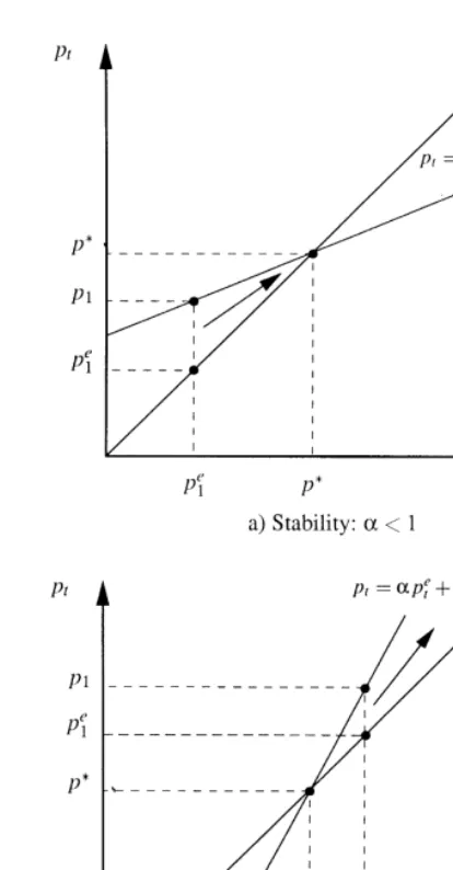
The stability condition a(1 may be interpreted as follows: Assume that
given a vector of parametersh
tand a realization of the exogenous variablesxt,
the expectation of the endogenous variable p%
t"f(xt,ht) (under) overestimates
the actual valuep
t. In this case, the learning algorithm (9) modi"es the vector of
parameters in a way that given x
t, there results a lower (higher) expectation.
Whether the repetition of this procedure will result in the correct rational
expectation givenx
t, depends on the value of the parametera.
With x
t given, the two cases can be distinguished: In case of Fig. 2a, with
a(1, the nature of the learning algorithm described above, implies that the
17AsJ(h) is a real symmetric matrix, all eigenvalues ofJ(h) are real.
Fig. 2. Learnability of correct expectations.
expectation errorp
t!p%t becomes smaller, whereas in case the of Fig. 2, with
a(1, it implies that this expectation error becomes larger. In the"rst case, an
algorithm based on this procedure may converge, while in the second case such an algorithm would never converge.
Proposition 3.4. If a!1'0, only (local) maxima of j(h) are stable stationary points of diwerential equation(10)and thus possible convergence points for learning algorithm(9).
This proposition states that the goal of the learning process will be completely
missed if a!1'0, because in this case the learning process steers towards
(local) maxima of the mean squared error j(h). But as is easily shown, this
implies that for tPR we have htPR, because for any parameter space
HLRq, any maximum ofj(h) will be on the closure of this set. In order to verify
this statement it must be shown that within any such set, there exists no
hHsatisfying the su$cient conditions for a maximum: a maximum ofj(h) implies
E[g(x)#e!(1!a)f(x,hH)]"0, because one element of hH represents a
constant term. Assuming that this element is the "rst element of hH, j(hH)
is a maximum only if we have for any su$ciently small k and
h@
0"hH{#(k, 0,2, 0) that j(hH)5j(h0). But because E[g(x)#e! (1!a)f(x,hH)]"0 we get j(h
0)"j(hH)#[(1!a)k]2'j(hH), such thatj(hH) can be no maximum.
Propositions 3.2 and 3.3 give necessary and su$cient conditions for a
para-meter vector hH3HLto be a locally stable "xed point of di!erential equation
(10). These conditions are thus necessary and su$cient for the probability that
htconverges to an element ofHLfor tPRto be nonzero. But this does not
imply thathtwill converge almost surely to an element ofHL. This will be the
case only if ahH3HLis a locally stable stationary point of di!erential equation
(10) and if additionally it is guaranteed thath
twill almost surely stay within the
domain of attraction of that stationary point in"nitely often. Corresponding
su$cient conditions for almost sure convergence of h
t towards an identi"ed
hHmay be formulated following Ljung (1977) by augmenting algorithm (9) with
a so-called projection facility.19However, in general nonlinear models it might
be an extremely di$cult task to formulate a projection facility ensuring almost sure convergence. Moreover, it is for the agents in the model to formulate a suitable projection facility. Thus, the use of such a projection facility in order to achieve almost sure convergence has been rightly criticized, e.g. by Grandmont and Laroque (1991).
4. A more general model
In the preceding section it was demonstrated that certain conditions have to be satis"ed to ensure that a learning process based upon a neural network may
converge towards}possibly approximate}rational expectations. It should be
noted, however, that approximate rational expectations are merely locally optimal, because they are local minimizers of the mean-squared prediction error. This means, that approximate rational expectations learned with the help of a misspeci"ed neural network may di!er substantially from correct rational
expectations}the label&approximate'says nothing about the actual distance
between approximate and correct rational expectations. Thus, one should refrain from interpreting the above-derived convergence results too much in favor of neural networks.
In more general nonlinear models, a similar problem arises, but here this problem has a new quality with serious consequences. In order to describe this problem in more detail, let us now consider the more general reduced form
p
t"G(p%t,xt)#et (13)
and suppose that all other assumptions regarding the model are still valid. Thus, the only di!erence is that reduced form (13) is not additively separable in the
expectation p%
t of the endogenous variable and a function of the exogenous
variablesx
t. Although this model is still a quite simple one, because the reduced
form (13) does not contain lagged endogenous variables, the analysis of learning
becomes now a more complicated one.20
The "rst problem regards possible rational expectations equilibria. Given reduced form (13), it is by no means guaranteed, that there exists a unique
function/(x
t) which is a rational expectations function, i.e. that satis"es
/(x
t)"E[G(/(xt),xt)#etDxt] almost surely.
Thus, it might be the case that there exist multiple equilibria. However, the possible existence of multiple rational expectations equilibria is not a speci"c feature of nonlinear models.
Another problem is that contrary to the model based on reduced form (1), the model based on (13) implies that the rest points of the di!erential equation associated with learning algorithm (9) will not coincide with local minima of the
mean squared errorj(h) (cf. Kuan and White, 1994b).
To see this, assume as before thatp%"f(x,h). The mean-squared errorj(h) is
then given by
j(h)"EMG(f(x,h),x)#e!f(x,h)N2
and the necessary condition for a minimum ofj(h) results as
£
hj(h)"2 EM£hf(x,h)[G(f(x,h),x) #e!f(x,h)][G
p%(f(x,h),x)!1]N"0, (14)
where G
p% denotes the partial derivative of G(p%,x) with respect to p%. But,
because p
t!f(xt,ht)"G(f(x,h),x)#e!f(x,h), the di!erential equation asso-ciated with the learning algorithm (9) is given by
hQ"EM£
hf(x,h)[G(f(x,h),x)#e!f(x,h)]N. (15)
A closer look at (14) and (15) reveals that the zeros of these two equations will in
general not coincide, because the term G
p%(f(x,h),x)!1 in (14) is neither deterministic nor independent from the other terms in (14). The zeros will coincide, if we have ahHsuch thatf(x,hH)"/(x) almost surely, because we then also have G(f(x,hH),x)#e!f(x,hH)"0 almost surely. Thus, if there exists ahHimplyingj(hH)"p2e, i.e. if the neural network is correctly speci"ed and is
able to give a perfect approximation of the unknown function/(x), thishHis
a rest point of di!erential equation (15). This is not true, however, for anyhthat
results only in a local minimum of j(h), because in such a case we have
G(f(x,h),x)#e!f(x,h)O0 almost surely and a zero of (15) will not correspond to a zero of (14), i.e. not correspond to a local minimum of the mean-squared prediction error. Only if the model has the property that the expectation regarding the endogenous variable enters the reduced form in a linear way such
thatG
p%(f(x,h),x)!1 is a constant, any local minimum ofj(h) will coincide with a rest point of (15).
Heinemann and Lange (1997) analyze neural network learning in a model with a reduced form given by (13). Assuming a correctly speci"ed
neural network, i.e. assuming that there exists a hH implying f(x,hH)"
G(f(x,hH),x) almost surely, they are able to derive a stability condition
for the learning process. The respective necessary condition is
E[G
p%(f(x,hH),x)!1](0, which is a generalization of the conditiona!1(0
derived from the simpler model considered above. But even if the neural network is correctly speci"ed, there may exist other stable rest points of di!erential equation (15). As has been shown above, contrary to the simple model based on reduced form (1), these rest points will not imply that
the mean-squared error j(h) is locally minimized. A related problem is that
di!erential equation (15) is not a gradient system. Therefore, the analysis of the local dynamics of the di!erential equation associated with neural network learning becomes much more complicated if more general reduced forms are considered.
approximation of the unknown rational expectations function cannot be
deter-mined a priori.21
5. Conclusions
In this paper it was demonstrated, how neural networks can be used to model
adaptive learning of}possibly rational}expectations. The analysis was based
upon a simple Cobweb model, where the rational expectations function is a nonlinear function of exogenous variables. Given such a true model, the assumption of a correctly speci"ed auxiliary model used by the agents to form the relevant expectations would imply an extraordinary a priori knowledge on the side of the agents. Clearly, the need of such a priori knowledge weakens any results concerning the potential learning of rational price expectations.
Because a neural network is able to approximate a wide class of functions to any desired degree of precision, it seems to be a suitable auxiliary model if the speci"c relation between exogenous variables and the resulting endogenous variable is unknown. It was shown that the possible convergence of a learning process based on a neural network towards rational expectations is governed by the properties of the underlying true model. In the simple case considered here, where the reduced form of the model is additively separable in the price expectation and a function of exogenous variables, the resulting stability condi-tion is equal to the condicondi-tion known from linear models and this stability condition holds irrespectively of the neural network to be correctly speci"ed.
But even if the neural network used by the agents is correctly speci"ed, i.e. if it contains enough hidden units to give a perfect approximation of the rational expectations function, learning does not need to converge to rational expecta-tions: if the mean-squared error of the price expectations is taken as a measure of the success of the learning procedure, it can be shown that agents might merely learn to form approximate rational expectations, implying a (local) minimum of this mean-squared error. Apart from the local optimality of approximate ra-tional expectations, nothing can be said regarding the actual distance between these expectations and rational expectations. This means that the performance of approximate rational expectations might be quite poor. Thus, the
conver-gence results achieved above should be read with caution}learning of rational
expectations is not a simple task even with the help of neural networks. It must be emphasized that the model considered in Section 3 is a very simple static model with an additively separable reduced form containing independent
and identically distributed exogenous variables. This simple structure implies that the resulting associated di!erential equation takes a form which can be analyzed quite easily and enables the derivation of a de"nite stability condition for the learning algorithm.
As shown by Kuan and White (1994a), it is in principle possible to analyze more general models using the same methodology, but with increased analytical expense. Although it is true that a correctly speci"ed neural network might be able to learn rational expectations even in more general models, the analysis of the reduced form considered in the previous section demonstrated that a mis-speci"cation of the neural network will have serious consequences: in general, the learning procedure yields parameter estimates implying expectations that are not even local minimizers of the mean-squared error.
Picking up a point already mentioned in the introduction, it becomes clear, that this objection can be raised against any procedure that is used in the learning process to approximate the unknown rational expectations function. Thus, the problem of misspeci"cation is neither solved by neural networks nor exclusively related to them, because it concerns all parametric auxiliary models upon which a learning process may be based. The only way to overcome the problem of misspeci"cation would be the use of nonparametric models as advocated by Chen and White (1994).
Acknowledgements
The author would like to thank Christiane Clemens, Mikko Packalen and anonymous referees of this journal for helpful comments and suggestions re-garding an earlier version of this paper.
References
Bray, M., 1983. Convergence to rational expectations equilibrium. In: Frydman, R., Phelps, E. (Eds.), Individual Forecasting and Aggregate Outcomes. Cambridge University Press, Cambridge, MA, pp. 123}132.
Bray, M., Savin, N., 1986. Rational expectations equilibria, learning and model speci"cation. Econometrica 54, 1129}1160.
Chen, X., White, H., 1994. Nonparametric adaptive learning with feedback. Discussion paper 94-21, University of California, San Diego.
Conlisk, J., 1996. Why bounded rationality? Journal of Economic Literature 34, 669}700. Cybenko, G., 1989. Approximation by superpositions of a sigmoidal function. Mathematics of
Control Signals and Systems 2, 303}314.
Fourgeaud, C., Gourieroux, C., Pradel, J., 1986. Learning procedures and convergence to rational-ity. Econometrica 54, 845}868.
Grandmont, J., Laroque, G., 1991. Economic dynamics with learning: some instability examples. In: Barnett, W., Cornet, B., D'Aspremont, C., Gabszewicz, J., Mas-Colell, A. (Eds.), Equilibrium Theory and Applications. Cambridge University Press, Cambridge, MA, pp. 247}273. Heinemann, M., Lange, C., 1997. Modellierung von Preiserwartungen durch neuronale Netze.
Diskussionspapier Nr. 203, Fachbereich Wirtschaftswissenschaften, UniversitaKt Hannnover. Hirsch, M., Smale, S., 1974. Di!erential Equations, Dynamical Systems, and Linear Algebra.
Academic Press, Boston.
Hornik, K., Stinchcombe, M., White, H., 1989. Multilayer feedforward networks are universal approximators. Neural Networks 2, 359}366.
Kelly, D., Shorish, J., 1994. Learning to be rational using neural networks. Carnegie Mellon University.
Kuan, C.-M., White, H., 1994a. Adaptive learning with nonlinear dynamics driven by dependend processes.. Econometrica 62, 1087}1114.
Kuan, C.-M., White, H., 1994b. Arti"cial neural networks: an econometric perspective. Econometric Reviews 13, 1}93.
Ljung, L., 1977. Analysis of recursive stochastic algorithms. IIIE Transactions on Automatic Control AC-22, 551}575.
Marcet, A., Sargent, T., 1989. Convergence of least squares learning mechanisms in self referential linear stochastic models. Journal of Economic Theory 48, 337}368.
MuKller, B., Reinhardt, J., 1990. Neural Networks: an Introduction. Springer, Berlin.
Salmon, M., 1995. Bounded rationality and learning; procedural learning. In: Kirman, A., Salmon, M. (Eds.), Learning and Rationality in Economics. Basil Blackwell, Oxford, pp. 236}275. Sargent, T., 1993. Bounded Rationality in Macroeconomics. Oxford University Press, Oxford. White, H., 1989. Some asymptotic results for learning in single hidden layer feedforward networks.
Journal of the American Statistical Association 84, 1008}1013.
White, H., 1990. Connectionist nonparametric regression: multilayer feedforward networks can learn arbitrary mappings. Neural Networks 3, 535}550.