International Review of Economics and Finance 9 (2000) 31–52
The effects of alternative fiscal policies on the
intertemporal government budget constraint
Marcelo Bianconi*
Tufts University, Department of Economics, 11 Braker Hall, Medford, MA 02155, USA Received 18 June 1998; accepted 24 February 1999
Abstract
This article presents the effects of alternative fiscal policies on the intertemporal government budget constraint when the time horizon of the policy maker varies. I show that the wealth effect associated with cuts in the skill-adjusted labor income tax rate improves the intertemporal budget balance, whereas the intertemporal substitution effect associated with the physical capital income tax rate deteriorates the intertemporal budget. Under plausible parameter values, the tax rate on skill-adjusted labor income cannot by itself balance the intertemporal budget at all horizons. 2000 Elsevier Science Inc. All rights reserved.
JEL classification:H3; H5; H6; E6
Keywords:Intertemporal government budget constraint; Endogenous growth; Human capital; Tax policy; Government spending
1. Introduction
This article addresses intertemporal budget issues relating to government expendi-ture and several distortionary taxes allowing for alternative time horizons for the policy maker. We use an endogenous growth sectoral model of physical and human capital accumulation along the lines of Stokey and Rebelo (1995) and Pecorino (1993) with the inclusion of government debt. This allows me to focus on intertemporal budget balance along the stationary balanced growth path. Three recent contributions by Ireland (1994), Bruce and Turnovsky (1999), and Pecorino (1995) pursue a similar line of analysis using a different framework. The first two papers do not include human
*Corresponding author. Tel.: 617-627-2677; fax: 617-627-3917. E-mail address: [email protected] (M. Bianconi)
capital and labor-leisure choice as is done in this paper, whereas Pecorino (1995)
does.1The differences in results are important. Including human capital and
labor-leisure choice makes a physical capital income tax cut increasethe long run budget
imbalance, contrary to the results of Ireland (1994) and Bruce and Turnovsky (1999). Second, extending Pecorino’s (1995) analysis I am interested in a quantitative assess-ment of the extent to which the horizon of the policy maker affects the design of alternative fiscal policies. In Ireland (1994), Bruce and Turnovsky (1999), and Pecorino (1995), the intertemporal budget constraint balances at the infinite horizon, whereas I consider alternative horizons and obtain a richer set of steady state balanced growth comparisons regarding the merits of each tax and/or government spending policy.
In general, I show that the wealth effect of human capital accumulation induced by neutral technical progress to the hours worked, discussed by Ben-Porath (1967) and Heckman (1976) among others, remains intact at the aggregate level, even though the stocks of physical and human capital vary across sectors. This is shown to be the main determinant of a possible improvement in the intertemporal government budget, independently of Laffer style effects on the tax revenues and intertemporal substitution
effects in consumption.2
In addition, I show that the shorter the horizon of the policy maker, the larger the government spending cut needed to balance the intertemporal budget. Policies to balance the intertemporal budget only based on tax rate cuts yield unrealistically high rates. In particular, it is shown that, under plausible parameter values, changes in the tax rate on skill-adjusted labor income cannot by itself balance the intertemporal budget. This result arises because of the interaction between worked hours and the economy-wide human-physical capital intensity, which basically determines the sec-toral human-physical capital allocations. Thus, decreasing the skill-adjusted labor income tax rate leads to an improvement of the intertemporal budget. The issue of tax incidence arises naturally in this framework. The physical capital income tax shifts the burden to skill-adjusted labor more heavily than vice-versa.
Another result of this paper is that a cut in government spending reduces the intertemporal budget imbalance more effectively relative to other alternatives. This can be coupled with a cut in the physical capital income tax, the skill-adjusted labor income tax, or the consumption tax, as long as it creates a “primary” surplus along the balanced growth path. But, the main ingredient is the cut in (net) non-utility enhancing government spending.
The article is organized as follows: section 2 presents the basic multi-sector model with physical and human capital accumulation; section 3 presents the intertemporal government budget constraint together with the measure of fiscal imbalance, the revenues from the productive factors, and its associated saving rate; section 4 presents the quantitative analysis, while section 5 concludes.
2. Macroeconomic model
of a consumption good, physical and human capital accumulation, and constant point-in-time returns to scale technologies. There is one nonreproducible factor input, the hours worked in market activities. The model is closely related to those in Stokey and Rebelo (1995) and Pecorino (1993) with the addition of government borrowing and lending as in Ireland (1994), Bruce and Turnovsky (1999), and Pecorino (1995). Since the framework is mostly standard, the presentation is brief.
The representative household solves the intertemporal problem [Eq. (1)]
Max e∞o U(c,,) e2rtdt
{c, ,, k,h, b} (1)
subject to the budget constraint [Eq. (1a)]
(1 1 tc) c 1Pk(k˙ 1 dkk) 1Ph(h˙ 1 dhh) 1b˙
< (12,)Phhw(1 2 th) 1Pkkr(12 tk) 1brb 2T (1a)
and given initial holdings [Eq. (1b)]
ko.0, ho .0, bo .0, (1b)
where all variables are in real terms, c is private consumption, , is leisure, r .0 is
the consumer subjective rate of time preference,kis the stock of physical capital held
by the consumer withdk denoting its rate of depreciation, h is the stock of human
capital held by the consumer withdhdenoting its rate of depreciation, bis the stock
of domestic short bonds issued by the government and held by the consumer,Pk is
the price of physical capital relative to the consumption good, which is taken as the
numeraire, Phis as well the relative price of human capital, w is the wage rate, r is
the rental rate of physical capital, rb is the return on government bonds, and T is a
lump-sum tax-rebate. In addition, agents face a set of flat tax ratesti, i 5c,k,h, on
consumption, physical capital income, and wages. The instantaneous utility function
U(c,,) is a well-defined concave function with partials Uc .0, Ucc ,0, U,.0.
The first order conditions for an interior solution to this problem are given by
Uc(c,,) 5 l (11 tc) (2a)
U,(c,,) 5 lPh hw(12 th) (2b)
r(12 tk)2 dk5 (P˙k/Pk)1 r 2 (l˙ /l) (2c)
(1 2,)w(12 th) 2 dh 5(P˙h/Ph) 1 r 2(l˙ /l) (2d)
rb5 r 2 (l˙ /l) (2e)
together with the transversality conditions
lim lk e2rt50; lim lh e2rt50; limlb e2rt5 0
t→∞ t→∞ t→∞ (2f)
marginal utility of wealth of the consumer. Eqs. (2a) and (2b) are marginal conditions for consumption and leisure, while (2c), (2d), and (2e) are arbitrage conditions equating rates of return across holdings of assets and consumption.
The production side of the model consists of three separate constant point-in-time returns to scale production technologies for physical capital, human capital, and
consumption using as inputs physical and human capital. Denote by G(kk,hk) the
production function for the production of physical capital, wherekkis the part of the
total physical capital stock used in the production of capital goods andhkthe part of
the total human capital also used in the production of capital goods. Likewise,H(kh,hh)
is the production function for human capital, andF(kc,hc) is the production function
for consumption goods. Then, profit maximizing behavior by competitive firms implies the following first order conditions
PkG1(hk/kk) 5PhH1(hh/kh) 5F1(hc/kc) 5rPk (3a)
PkG2(hk/kk) 5PhH2(hh/kh) 5F2(hc/kc) 5wPh (3b)
whereG1is the marginal physical product of physical capital in the capital good sector,
G2is the marginal physical product of human capital in the capital good sector, and
so on. Human/physical capital ratios are well defined by the constant returns to scale assumption. In closing the model, the government obeys a flow budget constraint consistent with its capacity to tax and borrow from the private sector, given a path
of government consumption expenditure denoted byg. This is given by
b˙5rbb1 g2 tkrPkk 2 thwPhh(1 2,) 2 tcc 2T. (4)
2.1. Balanced growth path
It is well known that the model presented above sustains endogenous long run growth. Along this balanced growth path, the interest rate and wages, and the relative prices of physical and human capital are constant. Under mild restrictions on
prefer-ences, leisure is also constant along the balanced growth path.3The common
endoge-nous growth rate, denoted byu, for c, k,h, b, andgalong the balanced growth path
is given by
u 5(1/s) [(12 tk)G1(hk/kk)2 dk2 r] (5a)
where 0 , (1/s) , ∞ is the consumer intertemporal elasticity of substitution in
consumption. Defining the momentary utility function of the representative consumer to be of the constant elasticity of substitution form,
U(c,,) 5{[cv(,)](12 s) 21}/(12 s)
where v(,) is well defined, and combining Eqs. (2), (3a), and (3b) with the equilibrium
in the three goods markets yields the general equilibrium balanced growth path for the endogenous variables: (hk/kk), (hh/kh), (hc/kc), ,, (c/k), (h/k), u, (kk/k), (kh/k), (kc/
k),r,w,Pk, andPh. Then, Eqs. (2c) and (2e) determinerb. These variables are solved
as implicit functions of the tax rates, government consumption expenditure as a share
Along the balanced growth path the lifetime welfare of the representative individual may be computed from Eq. (1), giving the formula
W 5 2{[c(o)v(,)](12 s)/{(12 s)[u(12 s) 2r]}} 2 [1/r(12 s)]. (5b)
Lifetime welfare is increasing in the growth rate, u, and under the usual conditions
that make the integral in Eq. (1) well defined, it is increasing in consumption and leisure.
3. The intertemporal government budget constraint
The final equation is the flow government budget constraint (4). Across balanced growth paths, budget deficits are perfectly correlated with the economy-wide growth
rateu. As is usual, lump-sum taxes guarantee the government’s intertemporal or long
run solvency. Integrating Eq. (4) forward and using the results above one obtains,
for every timet, the expression,
b(t)5 e(12 tb)rbt{b
o2[eto T(s) e2(12 tb)rbsds]
1ko[(g/k) 2 tkrPk2 thwPh(h/k)(12,) 2 tc(c/k)]
3[et
oe(u 1 dk2r(12 tk))sds]}. (6)
The measure of long run intertemporal solvency that I use is based on the consumer transversality condition given in Eq. (2f). However, I allow the government sector to
balance the intertemporal budget at any date T* in the future, where 0 < T* < ∞.
This provides a richer set of choices for several reasons. First, the process of fiscal reform, observed in OECD countries in general and in the U.S. in particular, is always
associated with some projected balance at a finite horizon, say T* periods into the
future. Second, as Auerbach (1994) shows, different branches of government have
different scenarios for the revenues and expenditures T* periods into the future,
leading to alternative estimates of the imbalances for a finite horizon. Third, T* →
∞may be only considered an upper bound on the long run budget imbalance since
in some cases actions can be taken at some t , ∞, which change the course of the
economy and alter the extent of the intertemporal imbalance. Fourth, a large body of political economy literature (Persson & Svensson, 1989; Chari & Cole, 1993 among others) shows how the timing of policies affects the pattern of government expenditures and its financing alternatives. To sum, allowing the horizon to vary gives me latitude to explore some more interesting fiscal policy choices.
Applying the condition in Eq. (2f) fort→T* and using Eq. (6) gives the formula5
(1/ko) {eTo* T(s) e2(12 tb)rbs ds} ;V(T*) 5
(bo/ko) 1{[(g/k) 2 tkrPk 2 thwPh(h/k)(1 2,) 2 tc(c/k)]
3(eu 1 dk2r(12 tk)T*2 1)/(u 1 d
k 2r (12 tk))}. (7)
this paper. The variableV(T*) is the value of lump-sum taxes as a share of the initial capital stock necessary to balance the intertemporal budget as a function of the time
horizon T*. As long as the implicit discount rate (u 1 dk 2 r(1 2 tk)) is strictly
negative, when T*→ ∞Eq. (7) converges to the usual intertemporal condition that
the present discounted value of lump-sum taxes equals the initial stock of debt minus
the present discounted value of future primary surpluses. Alternatively, asT* →0,
the variableV(T*) approaches (bo/ko), the initial stock of debt to capital ratio.6
The interpretation given to Eq. (7) is that a policy to “balance” the intertemporal
budget in 0<T*<∞periods requires that the other taxes—tk,th,tc, and/or government
consumption expenditure as a share of the capital stock, (g/k)—are chosen such that
V(T*)50. Any other government policy withV(T*).0, implies that in net terms
some form of lump-sum taxation is necessary to balance the budget for theT* horizon.
Alternatively, a policy that sustains V(T*) 5 0, for a T* horizon, requires that the
present discounted value of lump-sum taxes be 0, implying no net disbursements along
the horizon.7
It is useful to compute the partial derivative ofV(T*) with respect toT* from Eq.
(7), obtaining
]V(T*)/]T* 5 g eu 1 dk2r(12 tk)T* (8)
where g ; [(g/k) 2 tkrPk 2 thwPh(h/k)(1 2 ,) 2 tc(c/k)] is the budget deficit plus
lump-sum taxes minus interest payments on outstanding debt, as a share of the physical capital stock [see Eq. (4)]. This is some variant of the “primary” deficit. If this primary
deficit is positive, g . 0, then V(T*) is increasing in T*, ]V(T*)/]T* . 0, and to
needed to balance the long run budget is smaller than the initial stock of debt (bo/
ko) and the minimum requires T* →∞, or V(T*)5 (bo/ko) 2 g[1/ (u 1 dk 2 r(1 2
tk))]. In the knife edge case, where the measure of primary deficit is 0, g 50, then
]V(T*)/]T*50 independently of the horizon T*.
Studying alternative strategies for a balanced intertemporal budget at the horizon
T* involves the effects of taxes and expenditures on the economy-wide growth rate
and possibly the relative effects on the tax bases. These effects are associated with the possibility of “dynamic scoring”: a cut in the physical capital income tax rate stimulates the growth rate, expanding the tax base and improving the long run intertem-poral budget balance (see Ireland, 1994; Bruce & Turnovsky, 1999; Pecorino, 1995). On the other hand, along the balanced growth path, an increase in the economy-wide
growth rate induces an increase in the flow budget deficit in equation (4) because
along the balanced growth path,c,k,h,b, andgall grow at the common rate determined
by Eq. (5a). Thus, in this model there is no “static” scoring when comparing alternative
Table 1
The revenue as a share of total output generated by the tax on the return to physical capital is
Rk 5Pkrtk/[Pk(u 1 dk) 1Ph(h/k)(u 1 dh) 1(c/k) 1(g/k)] (9a)
where total output as a share of the capital stock is defined as
Y/k ;[Pk(u 1 dk) 1Ph(h/k)(u 1 dh) 1(c/k)1 (g/k)].
Similarly, the revenue from the tax on the return to skill-adjusted labor is
Rh 5(1 2,) Ph(h/k)wth/[Pk(u 1 dk) 1Ph(h/k)(u 1 dh)1(c/k) 1(g/k)]. (9b)
From Eqs. (9a) and (9b), note that changes in tax rates, government expenditures, and the implied change in interest and wage rates will impact government revenues through
the economy-wide growth rate, relative prices, and allocations (h/k) and (c/k).
A closed form analytic solution for the model presented may be only obtained in
some special cases.9My analysis compares economies along alternative steady state
balanced growth paths thus leaving aside transitional dynamics. I use numerical simula-tions as has been the norm in the related literature. See Lucas (1990), King and Rebelo 1990, Pecorino (1993, 1994, 1995), Ireland (1994), and Devereux and Love (1994) among others.
4. Quantitative analysis
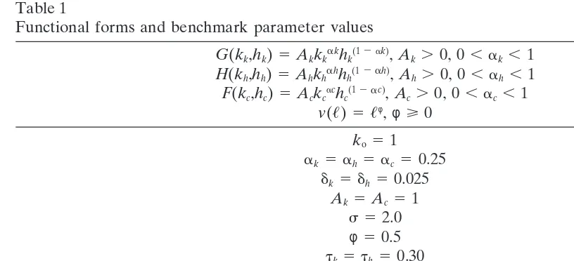
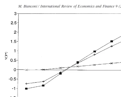
Fig. 1.V(T*): Tax rate cuts.
level of technology anda’s the physical capital shares. Preferences are CES as defined
above and the functionv(,) for leisure is also of the constant elasticity form, where
φ determines the consumer preference towards leisure. First, I calibrate the model
and solve for a benchmark balanced growth path. Following King and Rebelo (1990), I combine this base parameter set with chosen values for the before-tax real interest
rate, r 50.10, and the economy-wide growth rate, u 50.0125, and find the implied
values for r 50.02 andAh 50.1426 that support this allocation along the balanced
growth path. This base set implies that the sectoral human/physical capital ratios are identical, or (hk/kk) 5(hh/kh) 5(hc/kc); z, and the solution forz reduces to10
z5(h/k) (1 2,). (10)
The implied output-capital ratio in this benchmark allocation is Y/k 5 0.3133; thus
the initial stock of government debt is set atbo 50.15 giving a debt-output ratio of
about 48%, close to the current level in the U.S. economy.
Fig. 1 and 2 present the functionV(T*) evaluated at the base set and some alternative
values for taxes and government expenditure. At the benchmark balanced growth
path,g 50.0272.0, or the primary deficit is some 2.7% of the capital stock. Thus,
V(T*) is increasing in the horizonT* with a half-life of about 8.6 periods (years, for
example). In this case, the shorter the time horizonT*, the smaller the net disbursement
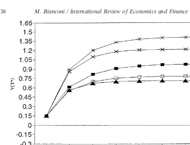
Fig. 2.V(T*): Government expenditure and tax cuts.
0.9857 or about 99% of the capital stock.11 Tables 2 and 3 show percentage point
changes from the benchmark allocations under alternative tax and government expen-diture combinations.
4.1. Tax rate cuts
If the physical capital income tax is cut in half to tk 5 0.15 and all the other
parameters are unchanged, Table 2 shows that the primary deficit, g, increases by
about 1.8%, and asT* →∞,V(T*) increases by 43.2% to about 142% of the capital
stock. There is no dynamic scoring as can be seen in Fig. 1 becauseV(T*) is above
the benchmark level for all T*. Alternatively, if the skill-adjusted labor tax is cut in
half to th 5 0.15 and all other parameters are unchanged, the primary deficit, g,
decreases by about 0.2%, and as T* →∞ V(T*) decreases by 19.7% to about 79%
of the capital stock. In this case, there is dynamic scoring in the sense that the present discounted value of lump sum taxes, as a share of the capital stock, decreases. The
important result, seen in Fig. 1, is that, whenth50.15,V(T*) is below the benchmark
case for all T*.0.12
The key to understanding these results is the effect on the economy-wide human/
physical capital intensity, h/k, and the sectoral human/physical capital intensities, z,
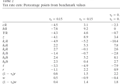
Table 2
Tax rate cuts: Percentage points from benchmark values
tc50.30
andzdecreases by 4.1%. Thus, the negative impact onh/kis greater than the positive
impact of more hours worked, and the sectoral intensities z fall. This leads to an
increase in the primary deficit, g, by 1.8% and a consequent deterioration of the
intertemporal budget. Whenthdecreases, leisure decreases by 4.9%, buth/kincreases
by 9.2%, and the sectoral intensities z increase by 8.9%. In this case, the positive
impact onh/kadds to the positive impact of more hours worked andzincreases. This
leads to a fall in the primary deficit of 0.2% and an improvement of the intertemporal
budget. Note also that when tk decreases, physical capital moves evenly from the
consumption sector to the physical and human capital sectors, 24.9%, 2.7%, and
2.2%, respectively. Alternatively, whenthdecreases, physical capital moves from the
consumption and physical capital sectors to the human capital sector,25.2%,20.1%,
and 5.3%, respectively. This asymmetry implies that the capital income tax cut makes the physical and human capital sectors less substitutes and more complements. How-ever, the human capital tax cut leads to a battle of the sectors as physical and human
capital sectors become more substitutes and less complements.13
In this general equilibrium framework, lifetime welfare is increasing in the growth
Table 3
Government expenditure and tax cuts: Percentage points from benchmark values
g/k50.04 g/k50.04
effect on the growth rate is too small to offset the loss in consumption and leisure,
and lifetime welfare falls by some 32%. When th decreases, consumption and the
growth rate increase, thus offsetting the loss from the decline in leisure, and welfare
rises by some 29%.14
The economic mechanism behind the effects of a cut intkcenters on the consumer
intertemporal substitution parameter. The implied moderate increase in the after-tax real return on physical capital induces the consumer to postpone current consumption
by increasing the saving rate on physical capital.15 Alternatively, a cut int
h leads to
a relatively larger increase in the after-tax real return on skill-adjusted labor and an
increase in the sectoral intensities,z. It has been pointed out, as early as Ben-Porath
(1967) and later by Heckman (1976), that human capital can operate as endogenous neutral technical progress by enhancing the productivity of hours worked. Thus, a
cut inthfunctions very much like an outward shift in the economy-wide production
possibilities surface, having little to do with intertemporal substitution in consumption
and more to do with aggregate wealth effects. As Table 2 shows,zincreases whenth
is cut leading to aggregate neutral technical progress.
Fig. 3.V(T*)50 with endogenous tax rates.
tk5 th50.15. Fig. 1 shows that there is no dynamic scoring, and the final impact on
V(T*) is intermediate betweentkandth. The economic rationale is that the
intertempo-ral substitution effect associated with tk dominates the wealth effect associated with
th. The last column presents the case where the two rates are set to 0, tk 5 th 5 0,
and replaced by a flat consumption tax,tc50.30. Because of the endogenous
labor-leisure choice, these two scenarios are obviously opposites. In fact, labor-leisure falls by
10.5%, and a combination of higher discount on future deficits,|u 1 dk 2r(12 tk)|
increases by 2.1%, and a minor increase in the primary deficit, up by 0.3%, leads to the best scenario for improved intertemporal budget balance in the class of tax rate alternatives. However, the general equilibrium effect on lifetime welfare is negative; the fall in consumption and leisure more than offsets the increase in the growth rate, and welfare falls by 8.6%.
4.2. Government expenditure and tax cuts
Fig. 4.V(T*) andth.
rates only, at all horizons T*. In the first column, g/kis cut by 3 percentage points,
representing an approximate 9% drop in government expenditure as a share of output. This is very effective in reverting the primary deficit into a primary “surplus,” since
g decreases by 2.8%. As T* → ∞, V(T*) decreases by 87.3% to about 11% of the
capital stock. In this case, as Fig. 2 shows, the longer the time horizonT*, the smaller
the net disbursementV(T*). Lifetime welfare,W, increases by some 15%, but there
is more private consumption and less private saving. There is a clear substitution of
government consumption for private consumption;c/k increases by 2.4%.
A cut in government expenditure coupled with a cut intk decreases the primary
deficit but does not produce a primary surplus since g falls only by 1.1%. AsT* →
∞, V(T*) decreases by 35.5%, but the longer the time horizon T*, the larger the
net disbursement V(T*). Lifetime welfare, W, decreases by 5.8%, with less private
consumption and more private saving due to the intertemporal substitution mechanism.
Whenthis cut, the battle of the sectors and wealth effects discussed above are again
observed. There is a primary surplus, g decreases by 3.0%, and as T* → ∞, V(T*)
decreases by 91.4% to about 7% of the capital stock. This is seen in Fig. 2 to be the
best scenario in terms of long run budget balance. Lifetime welfare,W, increases by
Fig. 5.V(T*)50 with endogenousg/k.
two tax rates are substituted by a consumption tax. These two cases are somewhat similar except for the effects on private consumption that are obviously diametrically opposed.
To sum up, within the long run intertemporal balance dimension, cutting government expenditure is the most effective tool. Given the neutral technical improvement gener-ated by human capital accumulation, a cut in government expenditure coupled with a cut in the skill-adjusted labor income tax rate provides the best policy choice for improving the intertemporal budget.
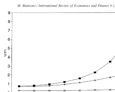
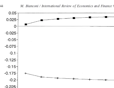
4.3. Policies to balance the intertemporal budget
The balanced intertemporal budget concept introduced above is a situation where
V(T*)5 0 along the balanced growth path. In this case, a surplus is generated that
pays the interest on the outstanding debt. Fig. 3 shows tax rates and welfare at different
horizonsT* for the cases where (a)tkis set endogenously forV(T*)50; (b)tcis set
endogenously forV(T*)50 whiletk5 th 50; and (c)tk5 thare set endogenously
forV(T*)5 0.
In all cases, balancing at a shorter horizon requires a higher tax rate, and as the
horizon gets longer the tax rates fall monotonically. The tax rates range from tc 5
Fig. 6.V(T*) andg/k.
T* in cases a and b but not in case c because the symmetric skill-adjusted labor tax
induces higher consumption of leisure and goods as T* increases. The tax on
skill-adjusted labor income,th, cannot by itself sustain a balanced budget withV(T*)50
along a balanced growth path under the base parameter set. The reason for this result
is depicted in Fig. 4, where it is shown thatth is increasing inV(T*) for all horizons
T* and more importantly,V(T*).0 for allthat all horizonsT*. In turn, there is no
value ofththat can bring the quantityV(T*) below its initial level equal to the initial
stock of government debt. The economics of this result are associated with the negative
wealth effect implied by the higher tax rate,th.
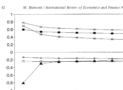
Fig. 5 and 6 show the case where government expenditure is chosen to make
V(T*)5 0 and the relationship between V(T*) and g/k for alternative horizons T*.
In Fig. 5, the values ofg/k range from 0.07% of the capital stock atT* 55 to 3.6%
atT*5200. Welfare decreases withT*, but the levels are comparable to the tax rate
cases. In Fig. 6, it is shown thatV(T*) is increasing in g/kfor all T*, butV(T*),0
for a wide range ofg/kvalues at different horizons, allowing government expenditure
to be consistent withV(T*)50. The figure also shows that whether the government
has a short horizon or a long horizon makes a difference for the change inV(T*). A
change ing/kat the short horizon induces a very small change inV(T*); the curve is
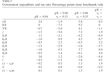
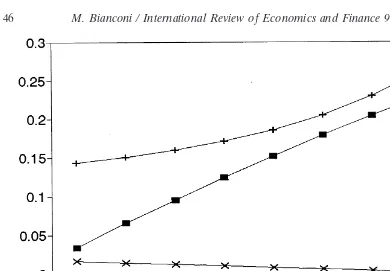
Fig. 7. Physical capital tax rate: Revenues and growth rate.
or 200 are much steeper. Thus, cutting g/k with the conjecture that the long run
intertemporal budget balances in a shorter horizon is shown to be incorrect.
4.4. Tax rates, tax bases, and the growth rate
Figs. 7–9 present simulations of alternative tax rates and the implied values for the factor revenues from Eqs. (9a) and (9b) and the economy-wide growth rate from Eq. (5a).
Fig. 7 shows that increasing the physical capital income tax rate,tk, induces gains
in the revenue from that factor. This is because the intertemporal substitution channel yields lower saving (capital) and thus a higher return, which coupled with the higher tax rate yields more revenue. The revenue on the other reproducible factor, human capital, also increases. It is important to note that there is an incidence issue here. Increasing the physical capital income tax rate shifts a lot of the burden to the other reproducible factor. This is one additional factor that explains why cutting the physical capital income tax rate leads to deterioration of the intertemporal budget. The growth
rate decreases only very slightly and turns negative at tk 5 80%.16 Fig. 8 shows the
case of the skill-adjusted labor income tax rate,th. The important differences are (a)
the revenue from skill-adjusted labor income first increases, and after aboutthclose
Fig. 8. Skill-adjusted labor tax rate: Revenues and growth rate.
capital income is decreasing in the human capital income tax rate, and there is no
shift of the tax burden to the other reproducible factor at least for th in the range
0–50%. In the range where th.50%, the revenue from skill-adjusted labor income
decreases because of the Laffer style effects, and at th 5 80%, the revenue from
physical capital income starts to increase. Thus, forth.50%, the burden shifts mildly
from skill-adjusted labor to physical capital. Both private saving rates decrease up to
th580%, increasing slightly afterwards. The growth rate decreases and turns negative
at about th 5 55%. Fig. 9 presents the symmetric case where tk 5 th. Again, the
revenue from human capital first increases, and after aboutthclose to 70% it decreases.
The growth rate decreases and turns negative at abouttk5 th550%.
The important result when Figs. 1, 4, and 8 are compared is that cutting the skill-adjusted labor income tax rate induces dynamic scoring independently of the Laffer style effects on the revenues from this factor—in other words, regardless of the level
of the tax rate. From Fig. 8 one would expect that cuttingthin the range 0.5, th,
0.9 would lead to dynamic scoring but not in the range 0, th ,0.5. However, Fig.
Fig. 9. Symmetric rates,tk5 th: Revenues and growth rate.
are small. This is shared by many previous authors, including Lucas (1990), King and Rebelo (1990), Pecorino (1993), and Stokey and Rebelo (1995).
5. Concluding remarks
intertemporal government budget, independently of Laffer style effects on the tax revenues and intertemporal substitution effects in consumption in this model.
A natural extension to this analysis is the quantitative consideration of transitional dynamics. When transitional dynamics are implemented, it breaks the perfect correla-tion between the flow budget deficit and the economy-wide growth rate. Then, one may distinguish between dynamic scoring and static scoring in this framework.
Acknowledgments
I thank the useful comments and discussions of J. Davies, Y. Ioannides, G. Metcalf, P. Pecorino, and S. Turnovsky on previous drafts of this paper and the constructive suggestions and comments of three anonymous referees for this journal. Any remaining errors or shortcomings are my own.
Notes
1. Ireland (1994) considers a convex one-sector growth model, whereas in Bruce and Turnovsky’s (1999) one-sector model the source of endogenous growth is government expenditure that enters the production function.
2. The endogenous labor-leisure choice is important because asymmetries in the effects of taxing physical versus human capital will arise in this case. See Pecorino (1993), Devereux and Love (1994), and Pecorino (1995) for a discussion. 3. Leisure is constant along the balanced growth path as long as preferences
guarantee that as income grows, substitution and wealth effects cancel out (see Lucas, 1990; Pecorino, 1993, 1995).
4. The balanced growth path is attained from arbitrary initial conditions for ko,
ho, bo, and go. It is well known that in the multi-sector endogenous growth
model in this paper, the arbitrary initial ratio (ho/ko) may not be the same as
the constant ratio along the balanced growth path. If this is the case, a period
of transitional dynamics, where h and k grow at different rates, leads the
economy to the balanced growth path, and government policy may distort this adjustment (see for example Caballe and Santos, 1993; Mulligan and Sala-i-Martin, 1993; Jones et al., 1993; Faiq, 1995; Devereux & Love, 1994). In this paper, I follow Lucas (1990), King and Rebelo (1990), Pecorino (1993, 1995), Stokey and Rebelo (1995), and abstract from transitional dynamics, restricting the analysis to the long run balanced growth path. This is done by assuming
thathois chosen endogenously to guarantee that the economy is in the balanced
growth path. Thus, there are no issues of time consistency of policy in this paper.
5. Technically, applying the transversality condition fort→T* is consistent with
consumer optimality to the infinite horizon (see for example Benveniste & Scheinkman, 1982).
consumer is indifferent between debt and lump-sum taxes given the path of distortionary tax rates.
7. Bruce and Turnovsky (1999) analyzeVfor the case whereT*→∞and interpret
it as a measure of sustainability of fiscal policy. Blanchard et al. (1990) present an alternative but related measure of sustainability of fiscal policy also used by Auerbach (1994).
8. Bruce and Turnovsky (1999) introduced the concepts of dynamic versus static scoring in their framework. Fullerton (1982), in a different framework, focused on the (uncompensated) elasticity of the labor supply with respect to changes in wages as a crucial parameter determining the possibility of static scoring. See also Pecorino (1995).
9. For example, if leisure is exogenously determined, under the restriction that the share of human capital in technology is the same across sectors, the model satisfies the dynamic nonsubstitution theorem of Mirrlees (1969). That is, the production possibilities surface is a linear plane, and there are no transitional dynamics across steady states. However, when leisure is endogenous the dy-namic nonsubstitution theorem fails, the production possibilities surface is strictly concave, and parameter changes can lead to transitional dynamics. See also Devereux and Love (1994).
10. In this case the relative prices are the same, that isPk 5Ph5 1.
11. In a different, nonoptimizing, model, Tobin (1986) shows that following the U.S. economy path of the early 1980’s, the nation’s capital stock would be depleted in about 11 to 12 years.
12. The dynamic scoring result for th is sensitive to the parameter of the leisure
function, φ. For example, if φ 5 2, the implied uncompensated labor supply
elasticity falls, and there is no dynamic scoring. However, for a plausible range
ofφ, it is shown below thatV(T*) is monotonically increasing inthand V(T*)
is strictly greater than zero for allthat different horizonsT*. This compromises
the use of th to achieve an intertemporal balance withV(T*)5 0.
13. In the paper by Devereux and Love (1994), transitional dynamics are considered
for the case where s 51. In that model there are small long run effects in the
sectoral allocations and large transitional effects. In my model there are no
transitional dynamics; thus the variations inhothat guarantee that the economy
is in the balanced growth path lead to large sectoral reallocations.
14. In Lucas (1990), the results are different because the production of human capital only requires human capital per se. In this paper, the production of the three goods require all reproducible and nonreproducible factors. Pecorino (1993) has the same production structure as the one used here, but assumes that all government expenditures are returned as lump sum to the consumer; thus the tax reforms are fully compensated. Note also that the effects of the wage tax cuts would be less dramatic if human capital were a partially, instead of fully, taxed activity. See also Jones et al. (1993), and Stokey and Rebelo (1995).
one capital income tax rate; thus they show that if the elasticity of intertemporal
substitution is large, say s , 1 [(1/s) . 1], then there is dynamic scoring in
their case. In Ireland’s (1994) convex one-sector model, there is also dynamic scoring arising from Laffer style effects in the tax bases. In my multi-sector model with human capital accumulation, there is no dynamic scoring,
indepen-dent of s.
16. The tax burdens mentioned are across steady state balanced growth paths and are uncompensated. The issue of tax incidence is discussed by Kotlikoff and Summers (1979) in a two-period model with human capital. However, their production function for human capital only requires raw hours as an input. See also Bernheim (1981) and Turnovsky (1982) for alternative dynamic analyses of tax incidence.
References
Auerbach, A. J. (1994). The U.S. fiscal problem: where we are, how we got here, and where we’re going. In S. Fischer & J. J. Rotemberg (Eds.),NBER Macroeconomics Annual 1994(pp. 141–175). Cambridge, MA: MIT Press.
Ben-Porath, Y. (1967). The production of human capital and the life cycle of earnings.Journal of Political Economy 75(Suppl.), 352–365.
Benveniste, L., & Scheinkman, J. A. (1982). Duality theory for dynamic optimizing models of economics: the continuous time case.Journal of Economic Theory 27, 1–19.
Bernheim, B. D. (1981). A note on dynamic tax incidence.Quarterly Journal of Economics 96,705–723. Blanchard, O. J., Chouraqui, J. C., Hagemann, R. P., and Sartor, N. (1990). The sustainability of fiscal
policy: new answers to an old question.OECD Economic Studies 15, 7–36.
Bruce, N., & Turnovsky, S. J. (1999). Budget policies, and the growth rate: “Dynamic Scoring” of long-run government balance.Journal of Money, Credit and Banking 31, 162–186.
Caballe, J., & Santos, M. (1993). On endogenous growth with human and physical capital accumulation. Journal of Political Economy 101,1041–1067.
Chari, V. V., & Cole, H. (1993). Why are representative democracies fiscally irresponsible? Federal Reserve Bank of Minneapolis Research Department Staff Report 163, August.
Devereux, M. B., & Love, D. R. F. (1994). The effects of factor taxation in a two-sector model of endogenous growth.Canadian Journal of Economics 27,510–537.
Faiq, M. (1995). A simple economy with human capital: transitional dynamics, technology shocks, and fiscal policies.Journal of Macroeconomics 17,421–446.
Fullerton, D. (1982). On the Possibility of an inverse relationship between tax rates and government revenues.Journal of Public Economics 19,3–22.
Heckman, J. J. (1976). A life-cycle model of earnings, learning and consumption.Journal of Political Economy 84,S11–S44.
Ireland, P. (1994). Supply-side economics and endogenous growth.Journal of Monetary Economics 33, 559–571.
Jones, L. E., Manuelli, R. E., and Rossi, P. E. (1993). Optimal taxation in models of endogenous growth. Journal of Political Economy 101,485–517.
King, R. G., & Rebelo, S. (1990). Public policy and economic growth: developing neoclassical implications. Journal of Political Economy 98,S126–S150.
Kotlikoff, L. J., & Summers, L. H. (1979). Tax incidence in a life cycle model with variable labor supply. Quarterly Journal of Economics 92,705–718.
Mirrlees, J. A. (1969). The dynamic nonsubstitution theorem.Review of Economic Studies 36,67–76. Mulligan, C. B., & Sala-i-Martin, X. (1993). Transitional dynamics in a two-sector model of endogenous
growth.Quarterly Journal of Economics 106,739–773.
Pecorino, P. (1993). Tax structure and growth in a model with human capital.Journal of Public Economics 52,251–271.
Pecorino, P. (1994). The growth rate effects of tax reform.Oxford Economic Papers 46,492–501. Pecorino, P. (1995). Tax rates and tax revenues in a model of growth through human capital accumulation.
Journal of Monetary Economics 36,527–539.
Persson, T., & Svensson, L. (1989). Why a stubborn conservative would run a fiscal deficit: policy with time inconsistent preferences.Quarterly Journal of Economics 104,325–345.
Stokey, N. L., & Rebelo, S. (1995). Growth effects of flat tax rates.Journal of Political Economy 103, 519–550.
Tobin, J. (1986). The monetary-fiscal mix: long-run implications.American Economic Review Papers and Proceedings May, 213–218.