isprsarchives XL 2 W2 99 2013

(1)

A NOVEL METHOD FOR AUTOMATION OF 3D HYDRO BREAK LINE GENERATION

FROM LIDAR DATA USING MATLAB

G. J. Toscano*, U. Gopalam and V. Devarajan

Dept. of Electrical Engineering, University of Texas at Arlington, Texas, USA, george.toscano@mavs.uta.edu, udaykiran.gopalam@mavs.uta.edu, venkat@uta.edu

KEY WORDS: LiDAR, Water body, Classification, Break lines, Histogram

ABSTRACT:

Water body detection is necessary to generate hydro break lines, which are in turn useful in creating deliverables such as TINs, contours, DEMs from LiDAR data. Hydro flattening follows the detection and delineation of water bodies (lakes, rivers, ponds, reservoirs, streams etc.) with hydro break lines. Manual hydro break line generation is time consuming and expensive. Accuracy and processing time depend on the number of vertices marked for delineation of break lines. Automation with minimal human intervention is desired for this operation. This paper proposes using a novel histogram analysis of LiDAR elevation data and LiDAR intensity data to automatically detect water bodies. Detection of water bodies using elevation information was verified by checking against LiDAR intensity data since the spectral reflectance of water bodies is very small compared with that of land and vegetation in near infra-red wavelength range. Detection of water bodies using LiDAR intensity data was also verified by checking against LiDAR elevation data. False detections were removed using morphological operations and 3D break lines were generated. Finally, a comparison of automatically generated break lines with their semi-automated/manual counterparts was performed to assess the accuracy of the proposed method and the results were discussed.

1. INTRODUCTION

Vast majority of the feature detection work appears to be in urban areas. Building tops, well defined fields, streets etc. are some of the more common features that are detected from overhead imagery and LiDAR. Our investigations unearthed very little work in the automated generation of rural features such as water bodies in wetlands – something that the NRCS is much interested in. Although manual and semi-automated approaches exist for some rural feature generation, these tend to be time consuming and expensive.

Water body detection is necessary to generate hydro break lines, which are in turn useful in creating deliverables such as TINs, contours, DEMs from LiDAR data. Surface water mapping is also essential in many applications such as monitoring of river corridor for natural hazard management (e.g. French, 2003; Brügelmann and Bollweg, 2004; Hollaus et al., 2005), surveying geomorphological change of floodplains (Thoma et al., 2005, Jones et al., 2007) and to improve understanding of wetland dynamics (Jenkins and Frazier, 2010).

Combining LiDAR elevation and intensity data gives better classification accuracy for water body detection (Antonarakis et al., 2008; Brzank et al., 2008; Höfle et al., 2009). By supervised fuzzy classification, Brzank et al. (2008) delineated water body in Wadden sea area, where low intensity and low elevation were given higher probability for the presence of water bodies. However, this method is not applicable to water bodies in land areas where water bodies do not necessarily have lower elevation. Therefore lower elevation does not increase the probability of finding water bodies on land. Especially in hilly regions, we can find water bodies at different elevations. Höfle et al., (2009) used a seeded region growing algorithm to delineate water surface from land. However, this method requires lots of pre-processing of LiDAR data such as dropout modelling.

In our method, we proposed a novel histogram analysis of LiDAR elevation data and LiDAR intensity data to

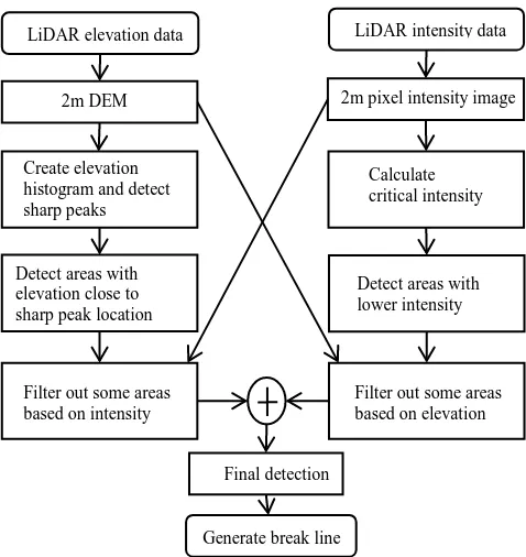
automatically detect and delineate water bodies with very little pre-processing. The surface of water body has the same elevation. So, if we create a histogram based on elevation, we generally notice a peak at the water surface elevation location. However, for small water bodies, this peak can get buried under elevation histogram of other places. Hence, LiDAR intensity data is essential to detect smaller water bodies. Thus we developed a novel algorithm that combines intensity and elevation in a unique fashion to detect small and large water bodies. The flow chart for the proposed auto hydro break line generation method is shown in figure 1.

Figure 1. Flow chart for the proposed auto hydro break line generation method

LiDAR elevation data LiDAR intensity data

2m DEM 2m pixel intensity image

Create elevation

International Archives of the Photogrammetry, Remote Sensing and Spatial Information Sciences,

(2)

2. DESCRIPTION

In this section, we describe the details of how we detected water bodies and generated break lines using both intensity and elevation data. We detected only the water bodies greater than half acre in size. At first we trained our algorithm for some training area in L’Anguille river basin, Arkansas, USA. Thereafter, we applied the algorithm in a test area in the same L’Anguille river basin. Here we describe our proposed method step by step for the test area.

2.1 Creating 2m DEM and 2m pixel intensity image

In this paper, we used rasterized digital elevation and intensity data to detect water bodies as point cloud based approach is complex. Point cloud based approach can admittedly give us more accurate result. However, if higher level of accuracy is needed, we can use point cloud data around the hydro break lines generated using the comparatively simpler raster based method.

At first we exported the .las file for a test area (where water body would be detected) to ASCII text format and read it in MATLAB. Then we divided the test area into 2m x 2m square grid. Using the elevation data of the last returns of the point cloud in each 2m x 2m square, we created a DEM. We used inverse distance weighted (IDW) interpolation technique to create the DEM. Squares from which no LiDAR return was recorded were given zero elevation and zero intensity value. From water bodies, probability of getting no LiDAR return is very high due to weak reflectivity of water at near infra-red wavelength as well as due to specular reflection from water surface.

To create the 2m pixel intensity image, each 2m x 2m square was represented by a single intensity value, which was determined by calculating the median of all the intensity values of the point cloud in that square area. Generally high relative variation of intensity is obtained from water surface and hence we took the median intensity from the LiDAR points in each square to represent the intensity value of that square in 2m pixel intensity image. The 2m DEM and 2m pixel intensity image for the test area are shown in figure 2 and figure 3.

Figure 2. 2m DEM of the test area in L’Anguille river basin

2.2 Creating histogram of elevation and locating sharp peaks

The range of elevation could be different for different areas. To create a histogram from elevation data, if we select the number of bins proportional to the range of elevation, then for different areas, the number of bins required would be different. However, we wanted to use equal number of bins for all the areas and we selected a large number 1024, as the number of bins for better resolution.

Figure 3. 2m pixel intensity image in log scale

In order to create a 1024 bin histogram from the 2m DEM (shown in figure 2), we multiplied the elevation values of the DEM by a ratio x where x = 1023/highest elevation value in the DEM. From the value of x, we defined a variable scale as

Scale = x, if 8 < x <25

= 8, if x ≤ 8 (1) = 25, if x ≥ 25

We calculated the scale for the test area to be 13.6293 using equation (1).

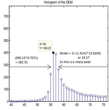
From the resulting DEM which now has elevation ranging from 0 to 1023, we rounded the elevation values to the nearest whole number and we got a modified 2m DEM. We created a 1024 bin histogram using this modified 2m DEM. We smoothed the histogram using a low pass filter with coefficients: [0.25, 0.5, 0.25] in order to minimize the effect of discretizing the elevation value and to make the histogram more reliable. The smoothed histogram is shown in figure 4. In figure 4, we showed only a portion of the histogram, where all the peaks are present.

From the histogram we calculated the peak locations, which are:

[295 284 268 255 238 225 216 207 198 189 180 166 156 146 137 56 1]

For all the peaks in the histogram, we calculated peak width to determine whether the peak is sharp or not. We found that the sharp peak locations in the histogram represent elevation,

Digital Elevation Model

median intensity image

(3)

Figure 4. Histogram of the modified DEM

around which it is highly probable to find water bodies. We calculated peak width by counting the number of bins around the peak with a height greater than 0.7071 times the peak height. If the width of a peak is less than 1.4142 times the scale (13.6293 for the test site), then we considered it to be a sharp peak. An example of sharp peak detection is shown in figure 5. The location of sharp peaks for the histogram in figure 4 are:

[198 189 56 1]

Figure 5. Peak width calculation for selecting sharp peaks

2.3 Calculating critical intensity

We calculated the median intensity value for the 2m pixel intensity image shown in figure 3 and found it to be 20. We found that if median intensity of a flat area is less than this median intensity value (20), then it is highly probable that the area is a water body. However, if we use this median intensity value as threshold to detect water bodies then many false detections could also occur. Hence, we determined a critical intensity value, which, if used as a threshold, will minimize the

number of false detections. The critical intensity value is less than or equal to the median intensity value. In the following paragraph, we describe how we calculated the critical intensity value using both the modified DEM and the intensity image.

For each sharp peak location, we detected the areas in the modified DEM with elevation ranging from (peak elevation –

scale/3) to (peak elevation + scale/4). For example, we detected

all the pixels which fall in the range �198− �13.6293

3 �, 198 +

�13.6293

4 �� for the peak at location 198. Using connected component analysis (4-connectivity based) we extracted connected pixels from the detected areas greater than half acre in size. For each of the connected areas, using the 2m pixel intensity image, we calculated the median intensity values which are shown in figure 6.

Figure 6. Median intensity values calculated for the connected areas with elevation close to the sharp peak elevations

Now in figure 6, starting from 20 (median intensity of the 2m pixel intensity image), we went down in descending order, looking for a sharp drop greater than a determined threshold (4 in this case) in median intensity values and found the first such drop from 18 to 12. We took the average of 18 and 12, i.e., 15 as the critical intensity value for the test site. We found that flat areas with median intensity less than the critical intensity are highly probable to be water bodies. We took the median intensity value of the 2m pixel intensity image as the critical intensity in cases where sharp drops were not found.

2.4 Detecting water bodies using elevation data

For each sharp peak location, we detected areas in the modified DEM the same way as we did while calculating critical intensity in section 2.3. We gave zero elevation to all the 2m x 2m squares from which no LiDAR return was recorded, so we got a sharp peak at zero elevation (bin #1) in the histogram. We added the areas having zero elevation to the areas detected around each sharp peak and performed a connected component analysis (4-connectivity based) to get probable water body areas. We rejected the areas less than half acre in size. We filtered out false detections using intensity data which is explained in the following paragraph.

We calculated the median intensity for each of those areas using 2m pixel intensity image. We rejected the areas with median intensity greater than 20 (median intensity of the 2m pixel intensity image). We took an 18-meter wide (18 meters is an optimum value, neither too narrow nor too wide) buffer surrounding each of the probable water body areas. For each of these surrounding areas, we calculated the median intensity using the 2m pixel intensity image. If the probable water body areas did not meet the condition: (median intensity of surrounding area) – (median intensity of probable area) < 3, we rejected those areas. For the rest of the areas, if any of the two following criteria was fulfilled, then we classified those to be water bodies:

a) Median intensity of probable area < critical intensity value b) Peak width for probable area < 4.

Width = 2< (1.4142*13.6293) or 19.27 So this is a sharp peak

(4)

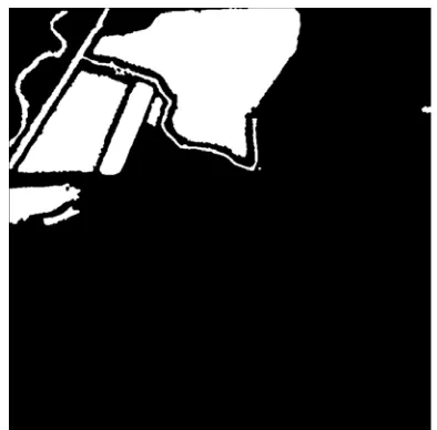
Water bodies detected using elevation data in the test area is shown in figure 7.

Figure 7. Water body detected using elevation data

2.5 Detecting water bodies using intensity data

Sometimes small water bodies might not get detected by the method we proposed using elevation data. The reason is that if the size of the water body is too small (which means that there are very few pixels with the same elevation), then the peak for that water body might either get buried in the histogram or not appear as a sharp peak. Hence, LiDAR intensity data should be used for detecting small water bodies. To detect water body from intensity data, we identified all the pixels in the 2m pixel intensity image with intensity less than the critical value. Using connected component analysis (4-connectivity based), we rejected areas less than 1/3 acre in size. However, we rejected all the connected areas less than half acre in size after merging the detections from intensity and elevation data.

For the rest of the low intensity connected areas, we performed a continuity test to filter out non-water body areas, making use of the fact that the water surface is generally continuous. We found voids or pixels which were not detected as part of the water bodies inside each of the connected areas. For each connected area, we summed all the void sizes and if any of the void size was found to be greater than 10 pixels, we took 10 as the maximum size of the void. Then for each connected area, we calculated the ratio of the total number of pixels to the sum of all void sizes. If the ratio was less than 14 then we rejected those areas as false detections. We filtered out more false detections using elevation data which is explained in the following paragraph.

We took an 18 meter wide buffer surrounding each of the probable water body and calculated the median elevation of the surrounding areas using the modified 2m DEM. We also calculated the median elevation of each probable water body. If the median elevation of surrounding area was greater than that of the probable water body by at least 3, then we considered those areas to be water bodies because the median elevation of a water body should be less than the median elevation of the surrounding areas. Water bodies detected using intensity data in the test area is shown in figure 8.

Figure 8. Water bodies detected using intensity data

2.6 Merging detections from elevation and intensity data

After detecting water bodies from elevation and intensity data, we merged the detections using a logical OR operation. We rejected areas less than half acre in size using connected component analysis and for the rest of the areas, we did the continuity test as described in section 2.5. Then using morphological operations, we closed small gaps or voids in the detected water bodies. The final detected water bodies are shown in figure 9.

Figure 9. Water body detected after merging detection from elevation and intensity data

2.7 Creating 3D break lines for detected water bodies

After detecting water bodies, we identified vertices from the edges of the detected water bodies to create vectors for the break lines. To generate 3D break lines, the median value of the elevation of each water body (calculated from 2m DEM) is chosen as the z value. 3D break lines for the detected water bodies are shown in figure 10. Though we used a vertical exaggeration factor of 10, the elevation difference is not clearly noticeable as all the water bodies have almost same elevation.

waterbody detected using elevation data

waterbody detected using intensity data

(5)

Figure 10. 3D break lines for water bodies shown in figure 9

3. RESULTS AND DISCUSSIONS

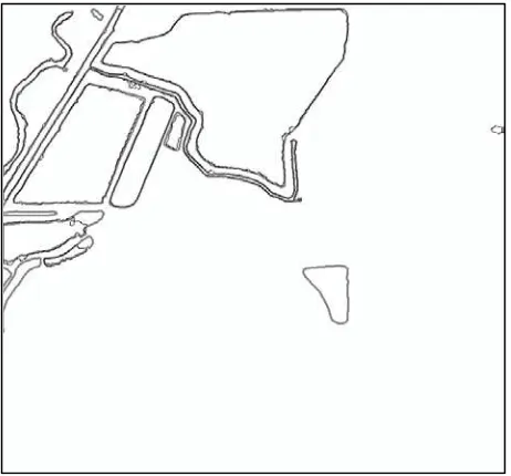
We compared the hydro break lines generated automatically by our method with the break lines drawn in semi-automated way. In figure 11, our break lines are shown by thin, dark lines and the break lines drawn in semi-automated way are shown by thick, light lines. From the comparison in figure 11, we found

Figure 11. Comparison between break lines generated in our fully automated method (thin and dark) and break lines drawn in

semi-automated method (thick and light).

that the auto generated hydro break lines closely matched with the break lines drawn in semi-automated way. However, the small water body in the bottom right corner was not detected by our method. The reason for this undetected water body was it’s small size and the LiDAR intensity values from this water body were not low enough to be classified as water body.

We applied our method in another test area in L’Anguille river basin and compared our auto generated break lines with the break lines drawn in semi-automated way, which is shown in figure 12. At the bottom right corner of the large water body, we found that the break lines did not match. And we also found a false detection at the bottom of the large water body. The false detection appears to have occurred due to the presence of a large number of dropouts in that area.

Figure 12. Comparison between break lines generated in our fully automated method (thin and dark) and break lines drawn in

semi-automated method (thick and light).

4. CONCLUSIONS

In general feature detection work in rural areas is somewhat sparse. In this paper, we used a novel method to detect and delineate water bodies using both LiDAR elevation and intensity data. Detecting water bodies from LiDAR data is a very challenging task due to high dropout rate and high intensity variation from water bodies. We have developed a novel automated approach to water body detection in a primarily rural area and therefore hydro break line generation. We found the break lines generated using our fully automated method closely matching with the break lines drawn in semi-automated way. As a future work, we propose the use of LiDAR point cloud data in the areas around the hydro break lines generated by our method to improve accuracy and remove much of the drudgery associated with the manual elements of this work.

References

Antonarakis, A.S., Richards, K.S., Brasington, J. 2008. Objects-based land cover classification using airborne LiDAR. Remote

Sensing of Environment, 112(6), pp. 2988–2998.

Brügelmann, R., & Bollweg, A., 2004. Laser altimetry for river management. International Archives of Photogrammetry,

Remote Sensing and Spatial Information Sciences, 35, pp.

234-239

Brzank, A., Heipke, C., Goepfert, J., Soergel, U. 2008. Aspects of generating precise digital terrain models in the Wadden Sea from lidar-water classification and structure line extraction.

ISPRS Journal of Photogrammetry and Remote Sensing, 63(5),

pp. 510–528.

French, J.R., 2003. Airborne LiDAR in support of geomorphological and hydraulic modelling. Earth Surface

Processes and Landforms, 28(3), 321–335

(6)

Höfle, B., Vetter, M., Pfeifer, N., Mandlburger, G., & Stötter, J., 2009. Water surface mapping from airborne laser scanning using signal intensity and elevation data. Earth Surface

Processes and Landforms, 34(12), pp. 1635-1649

Hollaus, M., Wagner, W., and Kraus, K., 2005. Airborne Laser Scanning and Usefulness for Hydrological Models. Advances in

Geosciences, 5, pp. 57-63

Jenkins, R.B. and Frazier, P.S., 2010. High-Resolution Remote Sensing of Upland Swamp Boundaries and Vegetation for Baseline Mapping and Monitoring. Wetlands, 30(3): pp. 531-540

Jones, A.F., Brewer, P.A., Johnstone, E., Macklin, M.G.. 2007. High resolution interpretative geomorphological mapping of river valley environments using airborne LiDAR data. Earth

Surface Processes and Landforms, 32(10), 1574–1592.

Thoma, D.P., Gupta, S.C., Bauer, M.E., Kirchoff, C.E., 2005. Airborne laser scanning for riverbank erosion assessment.

Remote Sensing of Environment, 95(4), pp. 493-501

Acknowledgement

This research was funded by NRCS (Natural Resources Conservation Service), Ft.Worth, TX. We are thankful to Mr. Steven Nechero, Collin McCormick and William Marken of NRCS for providing us LiDAR data along with useful technical guidance.