Sensitivity and moment analyses of head in
variably saturated regimes
B. Li* & T.-C. J. Yeh
Department of Hydrology and Water Resources, The University of Arizona, Tucson, AZ 85721, USA
(Received 7 February 1996; revised 1 September 1996; accepted 30 January 1997)
A numerical approach for approximating statistical moments of hydraulic heads of variably saturated flows in multi-dimensional porous media is developed. The approximation relies on a first-order Taylor series expansion of a finite element flow model and an adjoint state numerical method for variably saturated flows to evaluate sensitivities. This approach can be employed to analyze uncertainties associated with predictions of head of steady-state or transient flows in variably saturated porous media, with any type of boundary and initial conditions. Limitations of stochastic analytical methods such as spectral/perturbation approaches and the time-consuming Monte Carlo simulation technique are thus alleviated. An example is given to demonstrate the utility of the approach and to investigate the temporal evolution of head variances in a variably saturated flow regime. Results show that the fluctuation of the water table can have significant impacts on the propagation of the head variance. q1998 Elsevier Science Limited. All rights reserved.
1 INTRODUCTION
Hydrological properties of the subsurface generally exhibit a high degree of spatial variability at various scales due to heterogeneous nature of geological formations. Our knowl-edge of the spatial distribution of these hydraulic properties is usually limited and incomplete. As a result, our predic-tions of flow processes in the subsurface are subjected to uncertainties. To address the uncertainty associated with our predictions, stochastic modeling of flow processes in geo-logical media becomes necessary. In the past two decades, many stochastic analyses have derived statistical moments of hydraulic heads of flow processes either in fully saturated aquifers or unsaturated vadose zones. Few analyses have been directed toward the study of flow in an integrated system where part of the system is unsaturated (vadose zones) and part of it is fully saturated (groundwater reser-voirs). Since water usually percolates through the vadose zone from the land surface to the aquifer, a realistic stochas-tic analysis must consider the interaction between the vadose zone and the aquifer.
In general, given the statistical properties of hydraulic parameters, statistical moments of heads can be derived through analytical or numerical analyses1. Based on an
analytical first-order approximation, Dagan2,3 and Rubin and Dagan4formulated covariance functions of head in uni-form flow under fully saturated conditions. Bakr et al.5, Mizell et al.6, Gelhar and Axness7, Yeh et al.8–10 and Russo11employed a small perturbation approach and spec-tral analysis to derive the specspec-tral density functions and covariance function of head in saturated or unsaturated porous media. On the other hand, a Monte Carlo simulation was employed by Delhomme12 to examine the effect of measurements of transmissivity on the reduction of the head prediction variance; Smith and Schwartz13–15 ana-lyzed the condition effect of measurements of hydraulic parameters on head and solute arrival time based on Monte Carlo simulations. Recently, Harter and Yeh16used Monte Carlo simulation to investigate the effect of conduc-tivity and head measurements on the solute transport in the vadose zone.
Although numerical approaches are flexible, analytical methods are often preferred because they can provide expli-cit relationships between the statistical properties of hydrau-lic parameters and state variables associated with flow processes. However, the analytical approach generally has to rely on simplified assumptions, such as infinite flow domains, small variability of hydraulic parameters, and sta-tionary processes. While these assumptions are necessary to avoid complications in mathematics, they hardly reflect the All rights reserved. Printed in Great Britain 0309-1708/98/$19.00 + 0.00
PII: S 0 3 0 9 - 1 7 0 8 ( 9 7 ) 0 0 0 1 1 - 0
477
condition in field problems. For example, flow domains for groundwater are usually bounded by geological structures such as faults and different geological units. The upper boundary of groundwater reservoirs is generally associated with recharge or evapotranspiration that varies in time and space. In addition, the flow processes from vadose zones to aquifers are nonstationary since the degree of mean water saturation varies in space and time.
A numerical Monte Carlo simulation requires no such assumptions, except the specification of probability density functions for the hydraulic parameters. It can also be applied to either fully saturated, unsaturated or variable saturated flow in multidimensional media under steady or transient flow conditions. Furthermore, measurements of aquifer parameters can be easily incor-porated into the analysis of head moments without assuming any joint probability relationship between heads and conductivity values16. Nevertheless, the requirement of enormous CPU time, memory and storage spaces is the major drawback of the Monte Carlo simu-lation technique. In the analysis of multidimensional vari-ably saturated flow problems, this shortcoming becomes so severe that conducting such simulations is considered formidable.
Besides these analytical methods and Monte Carlo simu-lations, a first-order analysis through a Taylor series expan-sion of finite element or finite difference models has been used to derive approximate statistical moments of flow pro-cesses. Dettinger and Wilson17 employed the first-order approximation to analyze the intrinsic and information uncertainty associated with numerical models. Townley and Wilson18applied the first-order approach to investigate the uncertainty propagation during transient flow in aqui-fers. Hoeksema and Kitanidis19and Sun and Yeh20used the same approach to derive the covariance function of head. Overall, the advantage of this numerical first-order analysis over Monte Carlo simulations is that the covariance function of head can be explicitly related to the covariance functions of aquifer parameters. As a result, the statistical moments of head can be obtained without conducting a large number of simulations, and the CPU problems associated with Monte Carlo simulation can be avoided. On the other hand, since this first-order analysis employs numerical models into the formulation of covariance functions, it can examine either steady-state or transient flow with any type of boundary conditions as opposed to the analytical approach.
In this paper a first-order numerical technique for formu-lating statistical moments of head in transient, variably satu-rated flow regimes in multi-dimensional porous media is developed. We chose the first-order numerical analysis to avoid problems associated with the analytical methods and Monte Carlo simulations. A numerical adjoint state method was also employed to reduce the computational effort in the evaluation of sensitivities. Propagation of the head variances from a vadose zone to an aquifer was then investigated.
2 A FIRST-ORDER FORMULATION OF MOMENTS
Assume that three-dimensional flow in porous media under variably saturated conditions can be described by the fol-lowing equation:
(SsbþC(W))
]W
]t ¼
=·[K(W)=(Wþx3)] (1)
where:Wis the pressure head;Ssis the specific storage;bis
the index for saturation, and it is zero ifW,0, one ifW$
0;Cis the moisture capacity;xis the spatial coordinatex¼ {x1x2x3} in whichx3represents the vertical direction with
upward positive; t is time; and K is the unsaturated con-ductivity assumed to be related to the pressure head through the exponential model21:
K(W)¼Ksexp(aW)
whereKsandaare the saturated conductivity and the pore
size distribution parameter, respectively. Based on the exponential model, Russo22 presented a consistent form of thev–Wrelationship:
v¼(vs¹vr)(exp(0:5aW)(1¹0:5aW)) 2 2þmþvr
wherevris the residual water content andvsis the saturated water content.m, which is a parameter related to the tortu-osity of soils, is chosen to be zero in this study for math-ematical simplicity. The moisture capacity in eqn (1) is defined as dv/dW.
Equation (1) can be solved deterministically if the hydraulic parameters such as conductivity and soil retention parameters are perfectly known. However, field data have shown that these parameters vary significantly in the space field22–24. Delineating the spatial distribution of these para-meters at high resolutions is not generally possible. As a result, these hydraulic parameters may best be represented as stochastic processes in space1,25. If these parameters are assumed to be stochastic processes, eqn (1) becomes a stochastic differential equation and the head is, in turn, a stochastic variable characterized by its first and second sta-tistical moments. The first moment represents the average of all possible heads resulting from a given set of parameter values while the second moment reflects the effects of spatial variability in parameters (or uncertainties in our mean head prediction). In the following analysis, we will assume that saturated hydraulic conductivity (Ks and the
pore-size distribution parameter (a) are stochastic pro-cesses. Ss and m are assumed to be constant because of
their small spatial variabilities20,26.
2.1 Evaluation of first moments of head
written as:
(Cˆ(W)þbSs)]H ]t <
=[exp(F¹eAH)·=(Hþx3)] (2)
Notice that the mean flow eqn (2) has the same form as the original flow eqn (1) by recoveringKsandafromFandA.
With the mean eqn (2), theHfield can be determined if mean values of parameters such asKsandaare specified. However,
eqn (2) is only valid when the variability ofKsandais very
small, much less than one. For larger variances, higher-order terms should be included in the mean equation.
2.2 Evaluation of second moments of head fields
To address the uncertainty around the mean head field, it is necessary to derive the second moment associated with this mean field. To do so, the pressure head can be expanded in a Taylor series about the mean values of parameters (F and A). After neglecting the second- and higher-order terms, a first-order approximation of the pressure head can be expressed as
The above equation can also be written in a matrix form if the governing flow equation is discretized by a finite differ-ence or finite element approach:
{h}¼JhflF,A,H{f}þJhalf,A,H{a} (3)
where {} indicates the vector of the discretized variable;J is the Jacobian matrix that represents the derivative of head with respect to the parameters. Multiplying eqn (3) with transposes of {f}, {a} and {h} assumingfandaare uncor-related, and taking the expected value on both sides of the equation yields
Rhf¼JhfRff
Rha¼JhaRaa
Rhh¼JhfRffJhgT þJhaRaaJTha
(4)
where:RffandRaaare the covariance functions offanda, respectively; Rhh is the covariance function of head; Rhf denotes the cross-covariance functions betweenhandf;Rha is the cross-covariance ofhanda. The covariance functions of fandacan be specified as any one of the covariance mod-els27,28, although the exponential model is used in this study. Notice that Raa and any Jacobian matrix related to a will become zero if the medium is fully saturated since the para-meteradoes not exist in saturated flow equations.
eqn (4) was previously derived in the similar way for fully saturated flows by Dettinger and Wilson17 and Sun and Yeh20. As can be seen the covariance functions, Rhh, Rhf and Rha in eqn (4), are nonstationary due to boundary conditions and variably saturated flow regimes. They depend on locations, instead of the separation distance as in a second-order stationary process.
3 SENSITIVITY ANALYSIS OF HEAD BY ADJOINT STATE METHOD
The evaluation of the second moment of head fields requires the determination of the Jacobian matrices. The calculation of Jacobian matrices is often referred as the sensitivity ana-lysis since Jacobian matrices represent the changes of heads in response to the changes of hydraulic parameters. In our formulations, the sensitivity analysis is carried out by the adjoint state approach, in which the performance measure function is29,30:
P¼
Z
T Z
QG(W,f,a)dQdt (5)
whereWis the time-dependent pressure head of eqn (1).G is the state function which in this case is the pressure head at any given time and location.
Taking the derivative of the performance function with respect to any of the parameters, for instance,f, results in the marginal sensitivity of the performance functionP:
]P
The first term on the right-hand side of eqn (6) reflects the direct contribution form conductivity, while the second term represents the indirect influence of conductivity in the performance measure.
Equation (6) requires the evaluation of state sensitivity
]W/]f, which can be determined by using the adjoint state of eqn (1). To formulate the adjoint state equation, we differ-entiate eqn (1) with respect tofand obtain
]
Multiplying eqn (8) with an arbitrary functionf* and inte-grating it over time and spatial domains,TandQ, yields
Applying Green’s first identity to the third and fourth terms in eqn (9), using partial integration rule on the second term, and rearranging the first term, we obtain
Z
where: G represents boundary domains; Nt is a final or
terminal time; andqbis the flux through boundaries.
Add-ing eqn (10) to eqn (6), the marginal sensitivity of the performance measure becomes
To evaluate eqn (11), one must specify the state sensitiv-ityfor eliminate its contribution in eqn (11) by setting the coefficient in front off to zero. If choosing the latter, we have an adjoint state equation:
]G
subject to boundary conditions:
fpl
and the terminal condition:
fpl
t¼Nt¼0
wheref* is the adjoint state variable;G1is the first type of
boundary condition; G2 is the second type of boundary condition.
Notice that adjoin state eqn (12) is linear in terms of the adjoint state variable; it is valid for flow problems in fully saturated aquifers whenais equal to zero; for unsaturated flow,KandCare known and evaluated at the givenWvalue. If we choose G¼Wd(x ¹xk; t ¹ tk), an measurement or interest location where the sensitivity is requested, the state sensitivity at timetis evaluated as
]W
whereQkis the exclusive subdomain offkwhich is element k in this study since f is defined at each element. The change in the domain of integration from Q toQk is due to the fact thatKsis only related tofat elementkwhen the
simulation domain is discretized.
The evaluation of sensitivity of pressure head with respect to lna is obtained following the same procedure. In fact, the adjoint state equation for lna is identical to eqn (12). However, the state sensitivity is now computed by
]W
Notice that the adjoint state equation only needs to be solved once forfanda. However, the adjoint state equation under transient flow conditions needs to be solved back-wardly in time because of the terminal condition generated during the formulation of the adjoint state equation. The initial condition appeared in eqns (10) and (11) will be zero if initial pressure heads are prescribed. To avoid complica-tions in calculating the cross-covariance, the sensitivities of head are evaluated for each element since the aquifer para-meters such as the conductivity and pore size distribution parameter are specified for each element. However, the finite element model of eqn (2) computes heads at each node of the element. In order to evaluate the cross-covar-iance, the elemental value of heads is defined as the average of the nodal head values in that element. In the following example, the mean flow eqn (2) and the adjoint state eqn (12) are numerically solved using a Galerkin finite element technique31.
4 NUMERICAL EXAMPLE
evenly discretized into 203 20 elements and 441 nodes.
The values of hydraulic parameters and statistical para-meters are listed in Table 1. We assume that lnKsand lna
are uncorrelated. Fig. 1 displays the boundary and initial conditions for this analysis. Initially, the pressure profile is in hydrostatic status, with the total head equal to 3 cm everywhere. At time equal to zero (t¼0) the top boundary is suddenly switched to a constant pressure head of ¹8 cm, presenting a step input of water.
Here, our performance measure is defined as the head measurement at a given location along a streamline (curve C in Fig. 1) at different times. Based on this performance measure, the sensitivity value at an element thus represents the change of head at the given measurement location, with respect to a unit change in lnKsor lna at that element. A
positive value for the sensitivity with respect to lnKsat an
element means that an increase or decrease of lnKsat the
element will yield an increase or decrease in the head value at the measurement location. In contrast, a negative value for the sensitivity with respect to lna implies that an increase in lna will produce a decrease in head and vice versa.
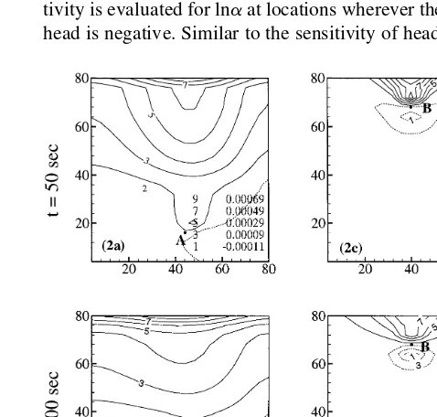
Fig. 2(a)–(d) show contours of head sensitivity values with respect to lnKsat two measurement locations, A and
B (see Fig. 1), fort¼50 and 100 s. Based on these figures, an increase of conductivity at the upstream area of the head measurement location (or a decrease of conductivity at the downstream) will increase the head at this location. Con-versely, the head will be reduced if the conductivity is decreased at the upstream or increased at the downstream. Overall, the magnitude of the positive sensitivity is greater than that of the negative one, suggesting that conductivities at the upstream area have stronger influence on the head value than those at the downstream. Such an asymmetrical sensitivity distribution in the vertical direction is attributed to the decrease in hydraulic gradient along the streamline
and the horizontal asymmetry is caused by the nonuniform flow. Boundary conditions also play an important role in the sensitivity behaviors of head with conductivity. Fig. 2(a) and (b) show that the highest sensitivity locates at the soil surface where the conductivity value determines the amount of water entering into the soil since a prescribed pressure head is given at this boundary. Sensitivity values for the head at location B (located in the unsaturated zone) are much greater than those for the head at location A (located in the saturated zone) at t ¼ 50 and 100 s. This can be attributed to the fact that the gradient in the unsaturated zone is greater than that in the saturated zone. It is found that the head in the saturated zone at A is influenced by conductivities over a larger area than the head at B in the unsaturated zone. Att¼100, the hydraulic gradient in the saturated zone increases and subsequently, the absolute head sensitivity for location A, in the saturated zone, increases. At the same time, the gradient near the soil sur-face decreases and the positive head sensitivity for B in the unsaturated zone decreases and the negative sensitivity values become more negative.
Fig. 3(a)–(d) show the sensitivity of head at locations A and B to lna. Since the pore size distribution parameter becomes effective only in the unsaturated zone, the sensi-tivity is evaluated for lnaat locations wherever the pressure head is negative. Similar to the sensitivity of heads to lnKs, Table 1. Hydrological and statistical parameters used in the analysis
Ks(cm/s) a(1/cm) j2f j2a lf,la( cm) vs vr Ss(1/cm) Covariance model forf
anda
0.009 0.05 0.3 0.1 20 0.3 0.0 0.0001 exponential
Fig. 1.Illustration of the flow domain, boundary and initial con-ditions for the test example.
Fig. 2.Sensitivity of head [(a) at location A andt¼50 s; (b) at location A and t ¼ 100 s; (c) at location B and t ¼ 50 s; (d) location B andt¼100 s] with respect to lnKs(solid lines
the sensitivity of head with respect to lnais gradient depen-dent. In addition, it depends on the product ofa and the mean pressure head,W[see eqn (14)]. Therefore, the sign of the sensitivity is opposite to that in Fig. 2 because the mean pressure head is negative under unsaturated conditions.
Another way to examine the relationship between head and hydraulic parameters is the cross-correlation analysis. The cross-correlation analysis provides useful information for the geostatistical inverse approach32,33. Fig. 4(a)–(d)
show the cross-correlation function between the head at the measurement locations, A, B and lnKsof all elements.
Note that the cross-correlation function at any specified location is determined by dividing Rhf by the product of standard deviations of h and f at the location. As can be seen the heads are always positively correlated with con-ductivity at all locations in the flow domain. This positive correlation is attributed to the prescribed constant head boundary conditions. An increase of conductivity at any location will yield an increase of infiltration rate from the soil surface, which in turn increases the head. Conversely, a decrease of conductivity will decrease the rate and the pres-sure head decreases. The cross-correlation increases slightly as more water enters the simulation domain.
Fig. 5(a)–(d) display the cross-correlation function between head and lna. Sincea does not exist in the satu-rated area, rha becomes zero below the water table. The general behavior of rhais similar to that of head and con-ductivity, except that negative correlation dominates all the area. The negative correlation is due to the fact that an increase of a is equivalent to a decrease of Ksunder the
given boundary conditions. As the infiltration continues, the cross-correlation of head with lnadiminishes, in contrast to the results in Fig. 4. Also shown in Fig. 5 is that pore size distribution parameter has less influence on head values than conductivity under this relative wet condition. These find-ings are consistent with that of Yeh and Zhang32.
It should be emphasized that the concept of sensitivity is a special case of cross-correlation analysis. In the sensitivity analysis, lnKsor lnais assumed to be spatially uncorrelated
and thus, the change of head at a given location reflects the change of lnKsor lnaof a particular element only. In other Fig. 3.Sensitivity of head [(a) at location A andt¼50 s; (b) at
location A and t ¼ 100 s; (c) at location B and t ¼ 50 s; (d) location B andt¼100 s] with respect to lna(solid lines represent
positive values and dash lines represent negative ones).
Fig. 4.Cross-correlation functions between head and lnKs[(a) at
location A andt¼50 s; (b) at location A and t¼ 100 s; (c) at location B andt¼50 s; (d) location B andt¼100 s].
words, the sensitivity represents a one to one relationship between the head at a given location and the parameter of a particular element. On the other hand, the existence of the spatial autocorrelation between two lnKsor lnavalues in the
cross-correlation analysis implies that a change of lnKsor
lna of one particular element can induce corresponding changes of lnKsor lnaof other elements. Therefore, when
a cross-correlationship is examined, the change of head at a given location reflects not only the effects of the change of lnKsor lnaat one element, but also that of the consequent
changes of lnKs and lna at other elements. More
specifi-cally, the cross-correlation function depicts the relationship between the head at a given location and the parameter of a particular element with the consideration of its relationship with parameters at other elements. This explains the reason why only positive cross-correlation exists in Fig. 4 while Fig. 2 depicts both negative and positive sensitivity values. That is, due to the spatial correlation, the large positive sensitivities has a strong influence on the cross-correlation between heads at locations A and B, and lnKs.
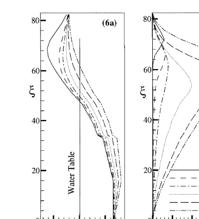
Covariances of head can be calculated using eqn (4). For conciseness, only the variance of head is discussed here. The head variance represents the uncertainty in our predic-tion of mean head or the head variapredic-tion around the mean, due to spatial variability in lnKsand lna. The mean pressure
head distributions along curve C at various times (50, 100, 120, 140, 160 and 180 s) are shown in Fig. 6(a) where the vertical axis, y, is the distance along curve C, measuring from the lower end of the curve. The head variance distribu-tions corresponding to the mean head distribudistribu-tions at differ-ent times are depicted in Fig. 6(b). These variance distributions take the form of a pulse and are always zero at the land surface since a constant head boundary is used (i.e. no uncertainty). The head variance grows from the upper boundary, reaches the maximum (peak variance), and then decreases to zero at the end of curve C where a constant pressure head is prescribed. At early times (t ,
160), the peak variance is found associated with the location of wetting fronts where the hydraulic gradient is the great-est; the position of the peak variance moves downward with the wetting front. When the wetting front arrives at the water table att¼140 s, this peak stays at the water table and does not further propagate through the saturated zone. Att ¼160 and 180 s, as the water table continues to rise, this peak head variance moves upward along with the water table and its magnitude also increases. Such findings suggest that the
water table will have significant impacts on the analysis of propagation of uncertainty or head variance in heteroge-neous porous media.
5 DISCUSSIONS
A flexible first-order numerical model is developed to study the sensitivity, the head variance, and cross-correlation functions of f and h (and h and a) for transient flow in variably saturated porous media. The results of the study provide insight to the effect of heterogeneity on transient, variably saturated flow. The flexibility of the approach stems from the fact that numerical models and the adjoint state method are used conjunctly. Numerical models pro-vide a simple means to treat any type of boundary and flow conditions. As a result, unlike the spectral method and other analytical methods, the assumption of stationarity is not required in the evaluation of statistical moments. The flex-ibility of our approach also stems from its ability to employ different types of K–Wandv–W relationships (other than the exponential model) in the analysis. In contrast, the ana-lytical methods are generally limited to the exponential model so that stochastic equations can be linearized.
Fig. 6. (a) Profiles of mean pressure head; (b) head variances along curve C at different times.
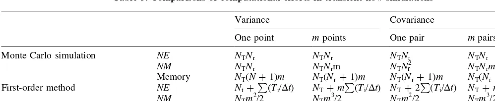
Table 2. Comparisons of computational efforts in steady-state flow simulations
Variance Covariance
One point mpoints One pair mpairs
Monte Carlo simulation NE Nr Nr Nr Nr
NM Nr Nrm Nr2 Nr2m
Memory (Nrþ1)m (Nrþ1)m (Nrþ1)m (Nrþ1)m
First-order method NE 2 (mþ1) 3 (mþ1)
NM m2/2 m3/2 m2/2 m3
The adjoint state method is computationally efficient. It allows us to evaluate the sensitivity only at the node of interest (such as locations of head measurements), instead of all the nodes as in other methods of sensitivity analysis. Additionally, the adjoint state equation usually retains the general form of the governing flow equation so that repeated finite element formulations can be avoided. In addition, the adjoint state equation for different parameters in the head sensitivity analysis remains the same; they only need to be solved once for all the parameters. In case of flow through variably saturated porous media, the governing equation is nonlinear, but the adjoint state equation is linear.
To compare the computational effort of our approach with that of the numerical Monte Carlo simulation, we eval-uate CPU time and memory needed for each approach. CPU time is usually proportional to the number of equations (NE) and the number of multiplications (NM). Memory is the computational space required to complete a calculation. Table 2 and Table 3 provide estimates of the computational efforts required for the calculating the second moment of head by both Monte Carlo simulation and our first-order approach. In these tables,m is the total number of nodes; Nr is the number of realizations needed in Monte Carlo
simulation;NTis the total number of time steps within the
simulation period;Tiis the time at outputI; andDt is the
time step. As can be seen our approach has the advantage of solving fewer equations over the Monte Carlo simulation if the number of points of interest is much less than the total number of nodes. This situation corresponds to many field problems where we have only sparse measurements. On the other hand, when a large number of points of interest are involved, the number of equations to be solved in our approach can be in the same order as that in the Monte Carlo simulation. However, in our approach the actual CPU time needed to solve one equation is much less than that in solving one equation in the Monte Carlo simulation. The reason is that the adjoint state equation is linear as opposed to the Richards equation. Moreover, the computa-tional grid size and time step can be much larger in the adjoint state method than those in the Monte Carlo simula-tion since the parameters considered in the adjoint state method are the constant mean. Therefore, adjoint state method requires less CPU time in solving equations. As for the number of multiplications and memory, Tables 2 and 3 show no significant difference between these two
methods, except that in the calculation of variance, Monte Carlo simulation conducts less NM than adjoint state method. Nevertheless, it can be concluded that our approach, in general, requires less computational effort than Monte Carlo simulation.
Another advantage of the first-order approach lies in its ability to derive co-conditional moments by incorporating measurements such as head and moisture content to inves-tigate the effect of conditioning32,33. In general, a co-condi-tional Monte Carlo simulation must build upon this first-order analysis.
In spite of the many advantages of our approach, we have to emphasize that it is based on a first-order approximation. The validity of the approximation is generally warranted if the variance of saturated hydraulic conductivity is less than one for saturated flow problems. For unsaturated flow pro-blems, the first-order approximation is valid if the variance of unsaturated hydraulic conductivity is much less than one16. At large variances, a higher order approximation or an iterative approach is required33,34.
Finally, application of our first-order numerical model to the analysis of propagation of head variance reveals some interesting findings that have not been reported previously. Our results provide quantitative evidences to show the effect of fluctuation of the water table. It thus becomes clear that vadose zones and aquifers must be treated as an integrated system to advance our understanding of flow and transport in the vadose zone and aquifers.
ACKNOWLEDGEMENTS
This research is funded by grants from NSF (EAR-9317009), USGS (1434-92-G2258) and NIEHS (ES04949). The support from the Environmental Management Science Programs of US Department of Energy under a subcontract (AV-0655#1) from Sandia National Laboratories is also acknowledged. Discussion on the computational effort with Dr Shu-guang Li is appreciated. We also like to thank the anonymous reviewers for their valuable suggestions.
REFERENCES
1. T.-C.J. Yeh, Stochastic modeling of water flow and solute transport in the vadose zone, in: A.I. Ei-kadi (Ed.),
Table 3. Comparisons of computational efforts in transient flow simulations
Variance Covariance
One point mpoints One pair mpairs
Monte Carlo simulation NE NTNr NTNr NTNr NTNr
NM NTNr NTNrm NTNr2 NTNrm
Memory NT(Nþ1)m NT(Nrþ1)m NT(Nrþ1)m NT(Nrþ1)m
First-order method NE NtþP(Ti/Dt) NTþmP(Ti/Dt) NTþ2P(Ti/Dt) NTþmP(Ti/Dt)
NM NTm2/2 NTm3/2 NTm2/2 NTm3/2
Memory NTm2/2 3NTm2/2 3NTm2/2 3NTm2/2
P
Groundwater Models for Resource Analysis and Manage-ment. Lewis Publishers, 1995, pp. 185–230.
2. Dagan, G. Stochastic modeling of groundwater flow by unconditional and conditional probabilities 1. Conditional simulation and the direct problem. Water Resources Research, 1982,18(4) 813–833.
3. Dagan, G. Time-dependent macrodispersion for solute trans-port in anisotropic heterogeneous aquifers.Water Resources Research, 1988,24(9) 1491–1500.
4. Rubin, Y. & Dagan, G. A note on head and velocity covar-iances in three-dimensional flow through heterogeneous ani-sotropic porous media. Water Resources Research, 1992,
28(5) 1463–1470.
5. Bakr, A.A., Gelhar, L.W., Gutjahr, A.L. & MacMillan, J.R. Stochastic analysis of spatial variability in subsurface flows, 1. Comparison of one and three-dimensional flows. Water Resources Research, 1978,14263–271.
6. Mizell, A.A., Gutjahr, A.L. & Gelher, L.W. Stochastic ana-lysis spatial variability in two-dimensional steady ground-water flow assuming stationary and nonstationary heads. Water Resources Research, 1982,18(4) 1053–1067. 7. Gelhr, L.W. & Axness, C.L. Three-dimensional stochastic
analysis of macrodispersion in aquifers. Water Resources Research, 1983,19(1) 161–180.
8. Yeh, T.-C.J., Gelhar, L.W. & Gutjar, A.L. Stochastic analysis of unsaturated flow in heterogeneous soils 1. Statistically isotropic media. Water Resources Research, 1985, 21(4) 447–456.
9. Yeh, T.-C.J., Gelhar, L.W. & Gutjar, A.L. Stochastic analysis of unsaturated flow in heterogeneous soils 2. Statistically anisotropic media with variable alpha. Water Resources Research, 1985,21(4) 457–464.
10. Yeh, T.-C.J., Gehar, L.W. & Gutjar, A.L. Stochastic analysis of unsaturated flow in heterogeneous soils 3. Observations and applications. Water Resources Research, 1985, 21(4) 465–472.
11. Russo, D. Stochastic modeling of macrodispersion for solute transport in a heterogeneous unsaturated porous formation. Water Resources Research, 1993,29(2) 383–397.
12. Delhomme, J.P. Spatial variability and uncertainty in ground-water flow parameters: a geostatistical approach. Water Resources Research, 1979,15(2) 269–280.
13. Smith, L. & Schwartz, F.W. Mass transport, 1. A stochastic analysis of macroscopic dispersion. Water Resources Research, 1980,16(2) 303–313.
14. Smith, L. & Schwartz, F.W. Mass transport 1. Analysis of uncertainty in prediction.Water Resources Research, 1981,
17(2) 351–368.
15. Smith, L. & Schwartz, F.W. Mass transport 3. Role of hydraulic conductivity in prediction. Water Resources Research, 1981,17(5) 1463–1479.
16. Harter, T. & Yeh, T.-C.J. Conditional stochastic analysis of solute transport in heterogeneous variably saturated soils. Water Resources Research, 1996,32(6) 1597–1609. 17. Dettinger, M.D. & Wilson, J. L First-order analysis of
uncer-tainty in numerical models of groundwater flow, Part 1. Mathematical development. Water Resources Research, 1981,17(1) 149–161.
18. Townley, L.R. & Wilson, J.L. Computationally efficient algorithms for parameter estimation and uncertainty propaga-tion in numerical models of groundwater flow. Water Resources Research, 1985,21(12) 1851–1860.
19. Hoeksema, R.J. & Kitanidis, P.K. An application of the geos-tatistical approach to the inverse problem in two-dimensional groundwater modeling. Water Resources Research, 1984,
20(7) 1003–1020.
20. Sun, N.-Z. & Yeh, W.W.-G. A stochastic inverse solution for transient groundwater flow: parameter identification and reliability analysis. Water Resources Research, 1992,
28(12) 3269–3280.
21. Gardner, W.R. Some steady state solutions of unsaturated moisture flow equations with applications to evaporation from a water table.Soil Science, 1958,85228–232. 22. Russo, D. Determining soil hydraulic properties by parameter
estimation: on the selection of a model for the hydraulic properties. Water Resources Research, 1988, 24(3) 453– 459.
23. Sudicky, E.A. A natural gradient experiment on solute trans-port in a sand aquifer: spatial varaiability of hydraulic con-ductivity and its role in the dispersion process. Water Resources Research, 1986,22(2) 2069–2082.
24. White, I. & Sully, M.J. On the variability and use of the hydraulic conductivity alpha parameter in stochastic treat-ments of unsaturated flow. Water Resources Research, 1992,28(1) 209–213.
25. Yeh, T.-C.J. Stochastic modeling of groundwater flow and solute transport in aquifers.Hydrological Processes, 1992,6
369–395.
26. S. Hanna, T.-C.J. Yeh, Estimation of co-conditional moments of transmissivity, hydraulic head, and vcelocity field. Advances in Water Resources, 1998, in press.
27. G. de Marsily,Quantitative Hydro Geology. Academic, New York, 1986.
28. Russo, D. & Bouton, M. Statistical analysis of spatial varia-bility in unsaturated flow parameters. Water Resources Research, 1992,28(7) 1911–1925.
29. Carrera, J. & Neuman, S.P. Estimation of aquifer parameters under transient and steady state conditions, 1. Maximum like-lihood method incorporating prior information. Water Resources Research, 1986,22(2) 199–210.
30. Sykes, J.F., Wilson, J.L. & Andrews, R.W. Sensitivity analysis for steady state groundwater flow using adjoint operators.Water Resources Research, 1985,21(3) 359–371. 31. Srivastava, R. & Yeh, T.-C.J. A three-dimensional numerical model for water flow and transport of chemically reactive solute through porous media under variably saturated condi-tions.Advances in Water Resources, 1992,15275–287. 32. Yeh, T.-C.J. & Zhang, J. A geostatistical inverse method for
variably saturated flow in the vadose zone.Water Resources Research, 1996,32(9) 2757–2766.
33. Zhang, J. & Yeh, T.-C.J. An iterative geostatistical inverse method for steady-flow in the vadose zone.Water Resources Research, 1997,33(1) 63–71.
![Fig. 3. Sensitivity of head [(a) at location A and t ¼ 50 s; (b) atlocation A and t ¼ 100 s; (c) at location B and t ¼ 50 s; (d)location B and t ¼ 100 s] with respect to lna (solid lines representpositive values and dash lines represent negative ones).](https://thumb-ap.123doks.com/thumbv2/123dok/3171793.1387909/6.709.51.293.83.313/sensitivity-location-atlocation-location-location-representpositive-represent-negative.webp)