Conference paper

(1)

ANALYZING THE EFFECTS OF SPATIAL RESOLUTION

FOR SMALL LANDSLIDE SUSCEPTIBILITY AND HAZARD MAPPING

O. E. Mora a, _{*, M. G. Lenzano} b_{, C. K. Toth} a_{, D. A. Grejner-Brzezinska} a

a

Department of Civil, Environmental and Geodetic Engineering, The Ohio State University, Columbus, OH – (mora.30, toth.2, grejner-brzezinska.1)@osu.edu

b

International Center for Earth Sciences, National Council of Scientific and Technological Research (CONICET), Mendoza, Argentina – mlenzano@mendoza-conicet.gob.ar

Commission I, WG I/2

KEY WORDS: LiDAR, landslide, feature, extraction, spatial, resolution, DEM

ABSTRACT:

Spatial resolution plays an important role in remote sensing technology as it defines the smallest scale at which surface features may be extracted, identified, and mapped. Remote sensing technology has become a vital component in recent developments for landslide susceptibility mapping. The spatial resolution is essential, especially when landslides are small and the dimensions of slope failures vary. If the spatial resolution is relevant to the surface features found in the landslide morphology, it will help improve the extraction, identification and mapping of landslide surface features. Although, the spatial resolution is a well-known issue, few studies have demonstrated the potential effects it may have on small landslide susceptibility mapping. For these reasons, an evaluation to assess the impact of spatial resolution was performed using data acquired along a transportation corridor in Zanesville, Ohio. Using a landslide susceptibility mapping algorithm, landslide surface features were extracted and identified on a cell-by-cell basis from Digital Elevation Models (DEM) generated at 50, 100, 200 and 400 cm spatial resolution. The performance of the landslide surface feature extraction algorithm was then evaluated using an inventory map and a confusion matrix to assess the effects of spatial resolution. In addition to assessing the performance of the algorithm, we statistically analyzed the surface features and their relevant patterns. The results from this evaluation reveal patterns caused by the varying spatial resolution. From this study we can conclude that the spatial resolution has an effect on the accuracy and surface features extracted for small landslide susceptibility mapping, as the performance is dependent on the scale of the landslide morphology.

1. INTRODUCTION

Spatial resolution is one of the fundamental characteristics of remote sensing (Chen et al., 2004; Vander Jagt et al., 2013). The spatial resolution defines the smallest scale at which surface features may be extracted, identified, and mapped from remote sensing technology. The spatial resolution may range from coarse (10 meters < ) to fine ( 1 cm > ) scales depending on the capabilities of the remote sensing technology used for mapping (e.g. spaceborne and airborne imagery, airborne and terrestrial LiDAR). Spatial resolution may refer to the ground sampling distance in an image or the grid size in a Digital Elevation Model (DEM), etc.

The information in a DEM is dependent on the spatial resolution (Chen et al., 2004). Spatial resolution exposes the surface features and patterns contained in a DEM. Improper choice of spatial resolution may lead to misinterpretation of the surface features, for example, coarse spatial resolutions will overlook fine scale surface features. For this reason, selecting an appropriate spatial resolution requires understanding the spatial scales of the surface features mapped.

An appropriate spatial resolution depends on surface complexity (Li et al., 2005), information desired and methods used to extract such information. To determine the appropriate spatial resolution, the scale of the available data, techniques for analysis, environmental settings, and objectives should be considered (Chen et al., 2004). For these reasons, evaluating the effects of spatial resolution is complex. In this paper, the impact

of spatial resolution, measured in DEM grid size on processing performance is investigated.

Many studies using remote sensing technology have explored the effects of spatial resolution (Irons et al., 1985; Turner et al., 1989; Benson and MacKenzie, 1995; Atkinson and Curran, 1995; Pax-Lenney and Woodcock, 1996; Qi and Wu, 1996; Schoorl et al., 2000; Chen et al., 2004; Lee et al., 2004; Claessens et al., 2005; Razak et al., 2011; Vander Jagt et al., 2013; Wang et al., 2013) to analyze landscape pattern (Turner et al., 1989; Qi and Wu, 1996) and landslide-susceptibility mapping (Lee et al., 2004; Claessens et al., 2005; Razak et al., 2011; Wang et al., 2013). Although, there have been studies focused on the effects of spatial resolution for landslide susceptibility mapping, to our best knowledge, none have focused on small failures.

Spatial resolution is an important component of landslide susceptibility mapping, especially when landslides are small and the dimensions of slope instability vary. The spatial resolution needs to be relevant to the scale apparent in the landslide morphology (Glenn et al., 2006). Spatial resolution affects all stages of landslide susceptibility mapping, from surface feature extraction to the classification of a DEM grid cell. Since the extents and surface features of small failures can be overlooked with coarse resolutions, an analysis is necessary to demonstrate the effects of spatial resolution on small landslide susceptibility mapping. However, landslide susceptibility is not only dependent upon the morphology; the geologic structure is

(2)

important as well as underground water flow. Nevertheless, in a geologically homogenous area the investigation is useful.

The objective of this paper is to demonstrate how spatial resolution affects small landslide susceptibility mapping at varying spatial resolutions, in addition to analyzing its effects on the geomorphological features. A 50 cm spatial resolution DEM was used to generate a series of coarser spatial resolutions at 100, 200, and 400 cm. Each DEM is classified using a Support Vector Machine (SVM). The classification and geomorphological features at each spatial resolution are examined to determine the effects of spatial resolution on small failures.

2. STUDY AREA AND DATA

2.1 Study Area

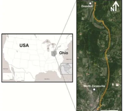
The study area is along the transportation corridor of state route (SR) 666 located at approximately Latitude: N39° 58’ 00”, and Longitude: W81° 59’ 00” beside the east side of the Muskingum River in Zanesville, Ohio. The area is characterized by high vegetation densities, stream and river channelling, and some residential development. Figure 1 presents an overview map of the study area. However, only a small section (see Figure 2) was used for the study. For more information regarding the study area refer to Mora et al., 2014.

Figure 1. Study area along SR-666, north of Zanesville, OH.

2.2 LiDAR Data

Airborne LiDAR is a remote sensing technology capable of penetrating the land cover and mapping surface models precisely. The airborne LiDAR data used in this research was acquired in the spring of 2012 with a point density of 5 pts/m2. The vertical accuracy of the points was assessed by the root mean square error (RMSE), which was 9 cm for soft- and 5 cm for hard-surfaces. The bare-earth, filtered from the LiDAR data, was subsequently used for this investigation. For more details in relation to the LiDAR data see Mora et al., 2014.

2.3 Landslide Geohazard Inventory

For the project area, a geohazard inventory and evaluation of mass movement affecting the transportation network was completed in 2006 by the Ohio Department of Transportation (ODOT) Office of Geotechnical Engineering (OGE). An

updated landslide inventory map was compiled in the summer of 2012. The updated landslide inventory compiled in 2012 was used for the investigation. A total of 80 landslides were mapped in the updated reference inventory map. Typical landslides affecting the road prism are: rotational, translational, complex, rockfall, debris and mudslides. The slopes for areas of instability range from 18° to 80°, in which the most frequently observed slope was 45°. The landslides described vary in age and have areas that range from 200 to 27,000 m2. For more information on the landslide Geohazard inventory map refer to Mora et al., 2014.

3. METHODOLOGY

The objective is to identify and map landslide surface features at varying spatial resolutions. This evaluation will determine the effects of spatial resolution on landslide susceptibility mapping and reveal patterns of its surface features.

3.1 Fine to Coarse DEM Generation

The coarse 100, 200, and 400 cm spatial resolution DEMs were built by resampling the base 50 cm DEM. The resampled DEMs were determined without interpolation due to the points lying at specific locations of the base DEM, where elevations were available, thus not requiring interpolation (Li et al., 2005). This technique can be regarded as a simple resampling method (decimation). However, if interpolation is required, the common interpolation methods used are: nearest point, bilinear and bicubic interpolation (Li et al., 2005).

3.2 Landslide Susceptibility Mapping

The landslide mapping technique characterizes and delineates the topographic variability of morphological features typical to landslides, including hummocky terrain, scarps and displaced blocks of material. The approach employs several geomorphologic features to analyze the local topography, specifically: the direction cosine eigenvalue ratios (λ1/ λ2and λ1/ λ3), resultant length of orientation vectors, aspect, roughness, hillshade, slope, a customized Sobel operator and soil type (Mora et al., 2013). A sample set extracted from the data is used as observations of landslide and stable terrain to train the supervised classification algorithm of Support Vector Machine (SVM). The trained SVM model is subsequently used to classify the LiDAR-derived DEM based on the extracted surface features. Then, as a post-classification step, flat terrain is filtered and classified as stable terrain. Consequently, a conditional dilation/erosion filter is applied to minimize misclassified locations by the SVM algorithm, in addition to suppressing noise and generating landslide susceptible regions (clusters). Landslide susceptible regions are then analyzed to map areas of potential landslide activity. The feature extraction algorithm used is described in detail in Mora et al., 2013. The parameters were used as described in the manuscript for all spatial resolutions.

3.3 Performance Evaluation

The performance evaluation was assessed by analyzing the resulting landslide susceptibility map to the independently compiled landslide inventory map. A common form to evaluate the performance of a landslide susceptibility model is to use a confusion matrix (Frattini et al., 2010). The model performance is analyzed by assessing the correctly and incorrectly classified

(3)

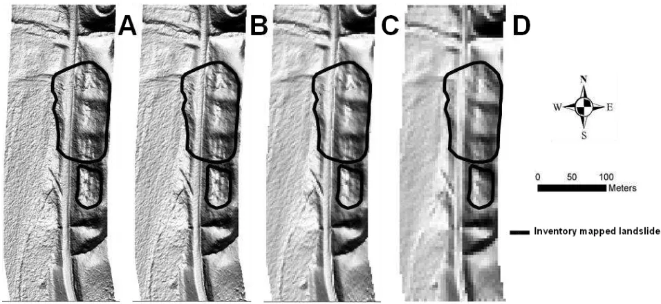
Figure 2. DEM maps with 50 (A), 100 (B), 200 (C), and 400 (D) cm spatial resolution. The areas outlined in black are the inventory mapped landslides.

landslide and stable areas, cell-by-cell. There are two types of errors involved in this type of accuracy assessment (see Table 1): Type I and Type II. Type I error is associated with the incorrect rejection of a true null hypothesis, while a Type II error is the failure to reject a false null hypothesis. The costs related to Type II error are usually larger than those of Type I (Frattini et al., 2010). Table 1 represents a two-class confusion matrix, as the one used.

Actual Class

Predicted Class

Landslide Stable

Landslide True Positive (+|+) False Negative (-|+), Error Type II Stable False Positive (+|-),

Error Type I True Negative (-|-) Table 1. Confusion matrix for performance evaluation

4. RESULTS AND DISCUSSION

Visibly, it is noticed in Figure 2 that the details in the DEM are lost as the spatial resolution decreases, meaning the surface features are no longer distinct in the DEM. One particular feature that looses detail is the transportation corridor. In the base (50 cm) DEM the corridor is easily depicted, but as the DEM becomes coarser it is no longer noticeably apparent, thus illustrating that surface features are lost as the spatial resolution decreases. This is due in part by selecting a landslide that provides adequate surface feature variety necessary to illustrate the objective of the study. In this paper, the term surface roughness refers to the topographic variability of the surface.

The statistics for each geomorphological feature were tabulated in Table 2 - Table 9. In the case of aspect and any surface feature extractor that uses any form of it in its evaluation, it is crucial to understand that flat surfaces will have high surface roughness caused by slight changes due to the variations of aspect on relatively flat surfaces. Any small change in aspect will cause the slope orientation, which is the compass direction a land surface faces to vary, thus mimicking landslide morphology. For this reason, it was determined that after

classification was performed on the DEM, flat terrain that is safe from landsliding should be filtered as stable. The threshold (15° ≥ Slope) was selected based on the unstable slopes for various types of mass movement described in Soeters and van Westen (1996) and those found in the study area. The surface features with this issue are: the direction cosine eigenvalue ratios ln(λ1/λ2) and ln(λ1/λ3), aspect, and the mean resultant length of orientation vectors (R) of the direction cosines.

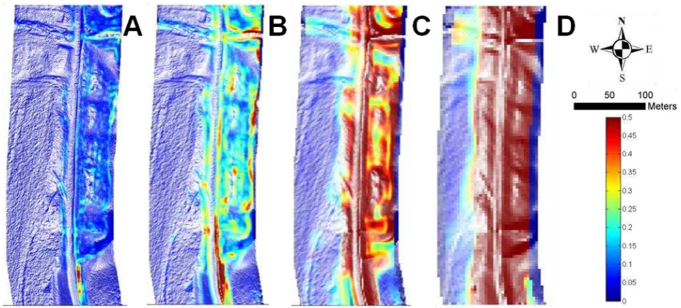
Topographic variability maps were made using the roughness surface feature extractor as shown in Figure 3. The surface roughness is shown to increase numerically along slope segments, however on relatively flat surfaces it tends to stay the same, as the spatial resolution decreases. These effects are caused by selecting to use the same parameters for all spatial resolutions. Therefore, the coarser the DEM the greater extents the local operator will cover when evaluating the surface roughness for each individual cell. This relationship is shown both visibly and quantifiably. The reason for this pattern is that as the spatial resolution decreases the DEM becomes coarser causing the local surface features to become dissimilar, however this may not be the case for all terrain types (e.g. flat surfaces). Therefore, the coarser the DEM, the more dissimilar the local surface features are within a local operator. This trend is only numerical, as in general the surface is smoothened over coarser spatial resolutions. This pattern is expected for both types of terrain due to the loss of detail. Although, the surface roughness does increase for both terrains the landslide terrain is shown to be rougher than stable terrain for slopes (15° ≥), except for the 400 cm spatial resolution where the surface roughness is similar in Table 2. For slopes (15° <) the surface roughness is similar for stable and landslide cells. The landslide terrain mean ranges from 6 to 91 cm for slopes (15° ≥) and 9 to 94 cm for slopes (15° <), while the stable terrain increases from 3 to 87 cm for slopes (15° ≥) and 9 to 92 cm for slopes (15° <), as the spatial resolution decreases. Landslides were shown to be rougher for cells having slopes (15° ≥), however for slopes (15° <) the mean surface roughness were similar.

The eigenvalue ratios ln(λ1/λ2) and ln(λ1/λ3) can be characterized as the higher the ratio the smoother the surface. In the case of the eigenvalue ratios ln(λ1/λ2) (see Table 3) it is

(4)

Figure 3. Surface roughness maps with 50 (A), 100 (B), 200 (C), and 400 (D) cm spatial resolution.

interesting to observe that the surface is rougher for stable cells for both slope categories, which is interesting as the surface is expected to be smoother, except for slopes (15° ≥) where it might be similar. However, an apparent pattern is observed that corresponds to the spatial resolution. The surface roughness of slopes (15° ≥) decreases with decreasing spatial resolution, compared to the surface roughness increasing for slopes (15° <) as the spatial resolution decreases, as expected. Additionally, the variations for landslide cells tend to decrease with decreasing spatial resolution.

The influence of spatial resolution on aspect is shown in Table 4. The pattern observed between slope cells (15° <) for both terrains is similar as the coarser the DEM, the higher the surface roughness. Slope cells (15° <) for both terrain types become smoother with decreasing spatial resolution. The surface roughness of slope cells (15° ≥) is higher than slope cells (15° <), as expected, which is caused by the high variations of flatter surfaces. The trend observed by slope categories is similar to that of the eigenvalue ratios ln(λ1/λ2), where slopes (15° <) become rougher with decreasing spatial resolution as opposed to slopes (15° ≥), where they become smoother.

In the case of the eigenvalue ratios ln(λ1/λ3) surface feature shown in Table 5, the surface roughness tends to increase as the spatial resolution decreases, except for landslide cells with slopes (15° ≥) where from the 200 to 400 cm spatial resolution the surface roughness decreases. Additionally, for stable cells with slopes (15° ≥) from 50 cm to 100 cm spatial resolution the surface roughness decreases, but then increases as expected. The stable cells have higher surface roughness than the landslide cells for slopes (15° <), however for slopes (15° ≥) the surface roughness is higher for landslide cells.

Hillshade (Table 6) displays the pattern expected as the DEM becomes courser the surface features become rougher as shown by the statistical mean and median. However, the landslide terrain is similar in surface roughness for both slope categories at each spatial resolution and the surface roughness increases minimally as the spatial resolution decreases. On the contrary, stable cells with slopes (15° <) are noticeably rougher than cells with slopes (15° ≥). The variations are smaller for landslide cells than stable cells for both slope types.

The surface feature of Sobel operator (Table 7) shows that the mean of stable cells are rougher for slopes (15° <). However, the variations are smaller. For slopes (15° ≥) the landslide cells mean are rougher than stable cells. Nonetheless, the variations of stable cells are smaller for spatial resolutions of 50 and 100 cm, while the variations are smaller for landslide cells at 200 and 400 cm spatial resolution. Landslide cells with slopes (15° <) and spatial resolution of 50 cm and 100 cm are rougher than landslide cells with slopes (15° ≥), this is vice versa for spatial resolutions of 200 and 400 cm. On the other hand, stable cells with slopes (15° <) are rougher than stable cells with slopes (15° ≥) for all spatial resolutions. Additionally, the variations tend to increase with decreasing spatial resolution for all cases.

Slope shown in Table 8 displays that for all cases the surface roughness increases with decreasing spatial resolution. The stable cells with slopes (15° <) are rougher than landslide cells with slopes (15° <). However, the mean of landslide cells with slopes (15° ≥) are rougher than stable slopes (15° ≥). The surface roughness of landslide cells with slopes (15° <) is rougher than landslide cells of slopes (15° ≥) at spatial resolutions of 50, 100 and 400 cm, this is not the case for the spatial resolution at 200 cm. For stable cells the mean is higher for slopes (15° <) than stable cells with slopes (15° ≥).

The strength of the mean vector R (Table 9) displays a unique pattern for all cases, where the surface roughness increases with respect to spatial resolution, but at the coarsest resolution the surface roughness decreases, except for landslide slopes (15° ≥) where the surface roughness decreases at the 200 cm spatial resolution. The distributions of the variations reveal the same pattern as that observed from the means. Additionally, all cases except the landslide cells with slopes (15° ≥) at a spatial resolution of 200 cm have a minimum of 0. Stable cells are rougher than their counterpart landslide cells for all cases, except for when landslide cells with slopes (15° ≥) are rougher than stable cells with slopes (15° ≥) at 100 cm spatial resolution.

(5)

Landslide Cells (15° < Slope) Stable Cells (15° < Slope)

Units: Meters .50 m 1m 2 m 4 m .50 m 1m 2 m 4 m

Mean 0.09 0.20 0.44 0.94 0.09 0.21 0.48 0.92

Med 0.08 0.19 0.43 0.91 0.08 0.19 0.44 0.85

STD 0.04 0.08 0.12 0.21 0.06 0.12 0.21 0.27

Min 0.02 0.04 0.11 0.52 0.01 0.03 0.09 0.51

Max 0.33 0.70 0.92 1.42 0.66 1.03 1.32 1.71

Landslide Cells (15° ≥ Slope) Stable Cells (15° ≥ Slope)

Mean 0.06 0.16 0.45 0.91 0.03 0.08 0.31 0.87

Med 0.05 0.15 0.46 0.92 0.02 0.05 0.22 0.96

STD 0.03 0.08 0.16 0.15 0.03 0.09 0.26 0.38

Min 0.01 0.04 0.11 0.61 0.00 0.02 0.03 0.21

Max 0.22 0.45 0.89 1.24 0.62 1.07 1.42 1.64

Table 2. Statistics of roughness surface feature.

Units: None .50 m 1m 2 m 4 m .50 m 1m 2 m 4 m

Mean 1.60 1.53 1.36 1.32 1.47 1.29 0.91 0.57

Med 1.64 1.54 1.39 1.32 1.56 1.33 0.88 0.56

STD 0.38 0.39 0.31 0.24 0.49 0.55 0.43 0.27

Min 0.10 0.17 0.42 0.53 0.01 0.02 0.02 0.05

Max 2.75 2.77 2.11 1.88 2.71 2.97 2.51 1.58

Mean 0.71 0.80 0.96 1.40 0.37 0.43 0.64 0.91

Med 0.68 0.72 0.97 1.40 0.24 0.29 0.57 0.86

STD 0.41 0.39 0.28 0.10 0.36 0.40 0.42 0.50

Min 0.00 0.01 0.17 1.25 0.00 0.00 0.01 0.08

Max 1.98 1.93 1.82 1.77 2.09 2.10 2.10 1.87

Table 3. Statistics of ln(λ1/λ2) eigenvalue ratios surface feature.

Units: ° .50 m 1m 2 m 4 m .50 m 1m 2 m 4 m

Mean 12.37 13.95 20.23 17.61 24.57 31.13 45.78 49.57

Med 9.65 10.05 12.40 13.68 10.68 14.04 35.62 42.55

STD 10.32 13.89 20.06 14.66 33.96 36.16 34.11 25.22

Min 3.27 3.38 3.73 6.41 2.80 2.10 2.13 10.39

Max 121.75 126.60 113.25 86.64 177.68 177.36 153.98 127.50

Mean 54.27 54.84 53.10 12.20 80.99 77.57 64.66 36.83

Med 43.42 41.74 55.97 12.38 89.21 88.12 70.41 22.68

STD 36.89 39.57 33.48 1.79 32.88 33.91 35.14 34.01

Min 5.92 5.43 7.11 7.18 5.42 4.91 3.72 6.73

Max 146.61 132.84 119.19 15.13 175.97 171.28 146.21 116.77 Table 4. Statistics of aspect surface feature.

Mean 2.15 2.06 1.86 1.71 2.14 2.01 1.69 1.49

Med 2.17 2.08 1.87 1.71 2.16 2.02 1.68 1.51

STD 0.31 0.34 0.29 0.14 0.43 0.48 0.39 0.24

Min 1.04 1.00 1.02 1.42 0.65 0.60 0.68 0.67

Max 3.25 3.00 2.68 2.07 3.46 3.59 2.99 1.95

Mean 2.11 1.89 1.64 1.71 2.33 2.37 2.08 1.88

Med 2.16 1.89 1.60 1.70 2.34 2.50 2.04 1.84

STD 0.41 0.44 0.34 0.10 0.36 0.50 0.71 0.69

Min 1.03 0.95 1.03 1.54 0.59 0.60 0.67 0.54

Max 3.25 3.00 2.72 1.96 3.58 3.57 3.77 3.01

Table 5. Statistics of ln(λ1/λ3) eigenvalue ratios surface feature.

(6)

Mean 0.08 0.08 0.09 0.10 0.09 0.10 0.13 0.19

Med 0.08 0.08 0.08 0.09 0.08 0.09 0.10 0.21

STD 0.03 0.03 0.02 0.02 0.05 0.07 0.07 0.06

Min 0.01 0.02 0.04 0.06 0.01 0.01 0.02 0.06

Max 0.24 0.19 0.17 0.19 0.42 0.38 0.33 0.30

Mean 0.07 0.08 0.08 0.09 0.06 0.06 0.07 0.12

Med 0.07 0.07 0.08 0.08 0.05 0.04 0.06 0.08

STD 0.03 0.02 0.02 0.01 0.03 0.04 0.05 0.10

Min 0.02 0.02 0.04 0.07 0.01 0.02 0.01 0.02

Max 0.18 0.15 0.14 0.13 0.43 0.38 0.35 0.32

Table 6. Statistics of hillshade surface feature.

Units: Meters .50 m 1m 2 m 4 m .50 m 1m 2 m 4 m

Mean 2.62 6.16 13.40 14.42 2.68 6.44 14.59 19.40

Med 2.33 5.73 13.90 20.08 2.27 5.78 13.53 24.16

STD 1.39 3.04 5.95 12.74 2.01 4.07 7.49 14.09

Min 0.00 0.00 0.00 0.00 0.00 0.00 0.00 0.00

Max 11.34 19.53 30.65 38.94 20.23 27.18 36.87 41.01

Mean 1.77 5.39 14.69 26.14 0.80 2.15 9.23 18.78

Med 1.39 4.86 14.10 25.69 0.48 0.93 6.81 23.13

STD 1.22 3.16 5.85 6.15 0.96 3.04 8.23 17.43

Min 0.00 0.00 4.01 0.00 0.00 0.00 0.00 0.00

Max 7.50 15.94 31.46 37.71 18.55 27.92 38.82 42.43

Table 7. Statistics of Sobel operator surface feature.

Units: ° .50 m 1m 2 m 4 m .50 m 1m 2 m 4 m

Mean 6.22 7.36 8.92 9.99 6.43 7.90 9.71 10.01

Med 5.74 6.92 8.55 9.85 5.80 7.20 8.95 9.63

STD 2.18 2.73 2.58 1.51 3.11 3.71 3.66 2.84

Min 1.86 2.23 3.05 6.49 1.47 1.54 2.61 5.22

Max 16.75 18.47 17.87 13.24 24.94 23.76 20.16 15.62

Mean 5.02 6.76 9.47 9.86 3.02 3.55 6.14 9.67

Med 4.44 6.44 9.53 9.71 2.46 2.34 4.51 10.16

STD 2.25 3.10 3.14 1.10 1.87 2.99 4.59 4.44

Min 1.36 2.01 2.68 7.59 0.43 0.86 0.91 1.82

Max 15.36 16.19 17.96 11.92 23.04 23.71 21.18 15.45

Table 8. Statistics of slope surface feature.

Mean 1.52 2.70 4.42 1.33 3.13 5.49 8.79 3.02

Med 0.41 0.71 1.65 0.00 0.66 3.25 9.22 0.00

STD 3.64 5.12 4.96 2.48 5.01 5.99 5.64 4.39

Min 0.00 0.00 0.00 0.00 0.00 0.00 0.00 0.00

Max 26.52 25.40 22.73 8.21 26.38 26.84 21.58 14.86

Mean 7.44 9.34 7.41 1.08 8.14 8.28 9.25 1.68

Med 6.21 7.64 7.74 0.00 7.81 7.31 8.55 0.00

STD 6.06 7.38 4.85 2.49 4.42 5.25 6.18 3.80

Min 0.00 0.00 0.21 0.00 0.00 0.00 0.00 0.00

Max 26.50 26.57 24.74 7.72 27.43 26.45 27.52 12.62

Table 9. Statistics of strength of mean vector R surface feature.

(7)

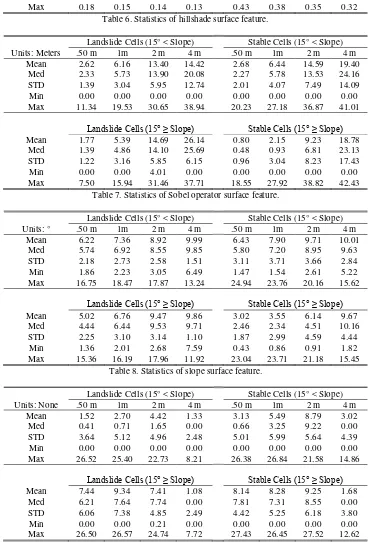
Figure 4. Classification using the SVM algorithm with 50 (A), 100 (B), 200 (C), and 400 (D) cm spatial resolution.

Analyzing the surface features extracted can help determine potential trends caused by spatial resolution. Some surface features may portray patterns that were anticipated and others might not. For this reason, it is essential to evaluate them statistically as unique similarities and trends can be found. From the evaluation, it was observed that the surface features displayed similar patterns amongst themselves at varying spatial resolutions, however some of the surface features displayed unique trends that were not expected. Most surface features behaved similarly as the spatial resolution decreased, some tended to generate rougher and other smoother surface features.

The classified landslide susceptibility maps generated at varying spatial resolutions are shown in Figure 4 and the performance evaluation was tabulated in Table 10. The accuracy statistics in Table 10 reveal that the algorithms performance decreases with respect to the spatial resolution, as expected. The performance of the true positive statistic signifying the landslide features that were classified correctly decreases from 35.71 to 0.00 %. This pattern signifies that the algorithm becomes incapable of distinguishing landslide and stable features due to the loss of detail in the terrain. The lower resolution of 400 cm has the worst performance as no landslide features are classified correctly and the highest resolution of 50 cm has the utmost performance. Although the 200 cm spatial resolution did not have the best performance, it did have the best precision. This may be due to the preservation of landslide features when resampling the DEM. Table 10 demonstrates a sharp drop in true positive classified cells from 200 to 400 cm spatial resolution. At the 400 cm spatial resolution all landslide morphological features are lost; therefore the classifier/model is unable to delineate the two types of terrain, thus explaining why no landslide terrain is classified correctly. Figure 4 shows that not only the size of classified landslide terrain varies with the spatial resolution, B and C show nearly completely different areas classified as landslides, but also the location differs significantly. This is due to the changes in spatial resolution. As the spatial resolution changes, so does the surface morphology. Therefore, not the same surface features will be preserved with decreasing spatial resolution.

Units: % 50 cm 100 cm 200 cm 400 cm

Accuracy 78.66 77.86 81.41 80.17

True Positive 35.71 17.42 13.86 0.00

False Positive 10.54 6.96 1.66 0.00

True Negative 89.46 93.04 98.34 100.00 False Negative 64.29 82.58 86.14 100.00

Precision 45.98 38.61 67.72 0.00

Table 10. Accuracy statistics of the classification algorithm.

The performance of the classifier demonstrates a strong dependency between the scale of the landslide surface features and the spatial resolution used to generate each DEM. For this reason, to maximize the performance of any landslide susceptibility model a spatial resolution performance evaluation is needed to determine a spatial resolution relevant to the surface features found in the landslide morphology. The proposed evaluation will minimize any issues pertaining to spatial resolution.

5. CONCLUSIONS

In this study, we applied a supervised classifier, which was previously shown to be an efficient model for small landslide susceptibility mapping. Four different spatial resolution DEMs ranging from 50 to 400 cm were generated using an airborne LiDAR data set. The objective was to assess how spatial resolution affects both surface feature extraction and small landslide susceptibility mapping with varying spatial resolution. It was determined that the base spatial resolution DEM for both data sets has the highest correctly identified landslide locations (true positive), while the lowest spatial resolution has the lowest. This demonstrates that small landslide susceptibility mapping can be performed more accurately with higher spatial resolution and we may conclude that the spatial resolution has an effect on the accuracy of small landslide susceptibility mapping, as the performance is dependent on the scale of the landslide morphology.

Spatial resolution is an important characteristic in small landslide susceptibility mapping as shown throughout this study. When generating DEMs for landslide susceptibility mapping it is important to know and understand the scale of the

(8)

landslide morphology in order to maximize the performance of the classifier. If the inappropriate spatial resolution is chosen, it may reduce the accuracy of the classifier. For this reason, it is suggested that an analysis is performed to understand the scale relevant to the landslide morphology before modeling the landslide surface. The optimal spatial resolution for landslide susceptibility mapping is determined by considering the accuracy, amount of data, and the scale of the landslide surface features.

ACKNOWLEDGEMENTS

The authors wish to acknowledge the support of Kirk Beach from the Office of Geotechnical Engineering of the Ohio Department of Transportation.

REFERENCES

Atkinson, P.M., and P.J. Curran, 1995. Defining an optimal size of support for remote sensing investigations. Geoscience and Remote Sensing, IEEE Transactions on, 33(3), pp. 768-776.

Benson, B.J., and M.D. MacKenzie, 1995. Effects of sensor spatial resolution on landscape structure parameters. Landscape Ecology, 10(2), pp. 113-120.

Chen, D., D.A. Stow, and P. Gong, 2004. Examining the effect of spatial resolution and texture window size on classification accuracy: an urban environment case. International Journal of Remote Sensing, 25(11), pp. 2177-2192.

Claessens, L., G.B.M. Heuvelink, J.M. Schoorl, and A. Veldkamp, 2005. DEM resolution effects on shallow landslide hazard and soil redistribution modelling. Earth Surface Processes and Landforms, 30(4), pp. 461-477.

Frattini, P., G. Crosta, and A. Carrara, 2010. Techniques for evaluating the performance of landslide susceptibility models. Engineering geology, 111(1), pp. 62-72.

Glenn, N.F., D.R. Streutker, D.J. Chadwick, G.D. Thackray, and S.J. Dorsch, 2006. Analysis of LiDAR-derived topographic information for characterizing and differentiating landslide morphology and activity. Geomorphology, 73(1), pp. 131-148.

Irons, J.R., B.L. Markham, R.F. Nelson, D.L. Toll, D.L. Williams, R.S. Latty, and M.L. Stauffer, 1985. The effects of spatial resolution on the classification of Thematic Mapper data. International Journal of Remote Sensing, 6(8), pp. 1385-1403.

Lee, S., J. Choi, and I. Woo, 2004. The effect of spatial resolution on the accuracy of landslide susceptibility mapping: a case study in Boun, Korea. Geosciences Journal, 8(1), pp. 51-60.

Li, Z., Q. Zhu, and C. Gold, 2005. Digital terrain modeling: principles and methodology. Boca Raton, CRC Press.

Mora, O.E., J.K. Liu, C.K. Toth, and D.A. Grejner-Brzezinska, 2013. Automatic landslide feature extraction from airborne LiDAR, Proceedings of the CaGIS/ASPRS 2013 Fall Conference, 29-30 October, San Antonio, Texas, (American Society for Photogrammetry and Remote Sensing, Bethesda, Maryland), unpaginated CD-ROM.

Mora, O.E., C.K. Toth, D.A. Grejner-Brzezinska, M.G. Lenzano, 2014. A probabilistic approach to landslide susceptibility mapping using multi-temporal airborne LiDAR data, Proceedings of the ASPRS 2014 Annual Conference, 23-28 March, Louisville, Kentucky, (American Society for Photogrammetry and Remote Sensing, Bethesda, Maryland), unpaginated CD-ROM.

Office of Geotechnical Engineering, 2006. Report of Findings: Geohazard Inventory and Evaluation: MUS-666-0.00, PID 79462, Ohio Department of Transportation, Columbus, OH, 137 p.

Pax-Lenney, M., and C.E. Woodcock, 1997. The effect of spatial resolution on the ability to monitor the status of agricultural lands. Remote Sensing of Environment, 61(2), pp. 210-220.

Qi, Y., and J. Wu, 1996. Effects of changing spatial resolution on the results of landscape pattern analysis using spatial autocorrelation indices. Landscape ecology, 11(1), pp. 39-49.

Razak, K.A., M.W. Straatsma, C.J. Van Westen, J.P. Malet, and S.M. De Jong, 2011. Airborne laser scanning of forested landslides characterization: terrain model quality and visualization. Geomorphology, 126(1), pp. 186-200.

Schoorl, J.M., M.P.W. Sonneveld, and A. Veldkamp, 2000. Three‐dimensional landscape process modelling: the effect of DEM resolution. Earth Surface Processes and Landforms, 25(9), pp. 1025-1034.

Soeters, R., and C.J. van Westen, 1996. Slope instability recognition, analysis and zonation, Landslides, investigation and mitigation. Transportation Research Board, National Research Council, Special Report, 247, pp. 129-177.

Turner, M.G., R.V. O'Neill, R.H. Gardner, and B.T. Milne, 1989. Effects of changing spatial scale on the analysis of landscape pattern. Landscape ecology, 3(3-4), pp. 153-162.

Vander Jagt, B.J., M.T. Durand, S.A. Margulis, E.J. Kim, and N.P. Molotch, 2013. The effect of spatial variability on the sensitivity of passive microwave measurements to snow water equivalent. Remote Sensing of Environment, 136, pp. 163-179.

Wang, L.J., K. Sawada, and S. Moriguchi, 2013. Landslide-susceptibility analysis using light detection and ranging-derived digital elevation models and logistic regression models: a case study in Mizunami City, Japan. Journal of Applied Remote Sensing, 7(1), pp. 073561-073561.