Validation of eddy flux measurements above
the understorey of a pine forest
E. Lamaud
∗, J. Ogée, Y. Brunet, P. Berbigier
INRA-Bioclimatologie, BP 81, 33833 Villenave d’Ornon Cedex, FranceReceived 7 January 2000; received in revised form 21 August 2000; accepted 1 September 2000
Abstract
Measurements of turbulent exchange in the understorey of a forest canopy are necessary to understand and model both the functioning of the lower stratum and its contribution to turbulent exchange at the whole canopy scale. Eddy covariance measurements of eddy fluxes just above the floor of a forest canopy must be thoroughly validated, given the particular conditions prevailing there. Our objective is two-fold: (i) check the overall quality of such eddy flux measurements through the analysis of the understorey energy balance closure and (ii) define quality criteria for each half-hourly sample, based on the residual term of the energy balance. A subset of the EUROFLUX data base, collected within a pine forest canopy in south-west France, was used for this purpose. During this experiment, all heat storage terms were carefully measured, which allowed the closure of the understorey energy balance to be rigorously tested. As in most experiments storage term measurements are not available, we also developed a method to estimate them, in order to apply the above-mentioned data selection method. The energy balance closure was found to be quite satisfactory (the slope of the sum of eddy fluxes and storage terms versus transmitted net radiation is 0.99, the intercept is less than 1 W m−2, r2is 0.94, there is no deviation from a linear trend). The
data selection procedure allows a fair description of the daily and day-to-day variation of turbulent fluxes while rejecting the most dubious data, whether experimental or estimated storage terms are used. This analysis proves the validity of eddy flux measurements in the lower part of the forest and offers tools for flux data selection, depending on the type of studies such data are intended for. © 2001 Elsevier Science B.V. All rights reserved.
Keywords: Eddy flux; Energy balance; EUROFLUX; Forest canopy; Understorey; Validation
1. Introduction
An increasing number of studies on energy and mass exchange between forest canopies and the atmosphere have been conducted over the past few years, in order to understand both forest functioning and the role of forests as sinks or sources of atmospheric pollutants. Although most studies have focused on carbon dioxide
∗Corresponding author. Tel.:+33-5-56843128;
fax:+33-5-56843135.
E-mail address: [email protected] (E. Lamaud).
and water vapor exchanges (Grace et al., 1995, 1996; Jarvis et al., 1997; Malhi et al., 1998), the interest for pollutants like ozone has grown during the past decade (Lamaud et al., 1994; Coe et al., 1995; Munger et al., 1996; Carrara et al., 2000).
One important difference between the forests and other vegetative surfaces is the presence of an under-storey, which contributes to the overall exchange of mass and energy. Until recently, forests have been considered as a whole and the specific role of the understorey was not taken into account. Thus, forest-atmosphere exchanges have often been
modelled using a “big-leaf” approach. For a given site, this model may provide accurate results if the processes occurring in the understorey and the over-storey are well coupled. This is not always the case. Also, a comparison between two sites may lead to erroneous interpretations if existing differences be-tween their understoreys are not taken into account. For example, Lamaud et al. (1996) showed that the differences observed between two pine forest plots resulted both from differences in the leaf area index of the overstoreys (3.5 versus 2.1) and from differ-ences in the understoreys (graminae versus ferns). Furthermore, as the processes involved in the transfer of the various scalars (water vapor, CO2, ozone) may
be different, the ratio of the corresponding fluxes between the overstorey and the understorey gener-ally differ. For example, more than 50% of day-time ozone deposition was found to occur on the under-storey, whereas only about 25% of the total exchange of water vapor resulted from understorey evaporation (Carrara et al., 2000). Lastly, as the vegetative cycles of the overstorey and understorey are different, es-pecially in coniferous forests, measurements cannot be performed throughout the year without taking into account the two layers separately.
In the recent years an increasing number of articles have been specifically considering the understorey (Baldocchi and Vogel, 1996, 1997; Blanken et al., 1997). The eddy covariance method is generally used to estimate the turbulent fluxes above the forest floor, as it is above the forest canopy itself. However, using this method in the lower part of the forest should be subject to much caution because the underlying hy-pothesis are generally not valid in the conditions pre-vailing there (low wind speed, strong heterogeneity, intermittent turbulence).
A thorough validation of turbulent flux measure-ments is therefore a necessary step in such studies. For this, energy balance closure represents a power-ful test for eddy flux measurements since it may allow the experimental data set to be validated on a mean basis, but also the most reliable data to be selected by rejecting spurious half-hourly values that do not per-mit the energy balance to be closed in a satisfactory way. The severity of this constraint must be modulated, depending on the objectives of the work.
Ecophysiological studies do not require as high a degree of accuracy in eddy flux measurements as
turbulence studies do. It is generally sufficient to be able to describe the relevant processes at the scale of several days, in order to assess the evolution of energy and mass transfer resulting from changes in environmental conditions. At daily scale, the data set must essentially allow one to describe the evolution of the processes between day and night and through the day as a consequence of stomatal activity and possible changes in dynamic (wind velocity and di-rection) and radiative (clear or cloudy) conditions. In this case, a rejection of the most spurious data, like occasional peaks in eddy flux measurements, is sufficient to provide an adequate data set. A severe selection may strongly reduce the use of the data set, as only “ideal” conditions (strong winds, clear days) can be studied. However, for specific analysis of tur-bulent transfer (involving spectral analysis, analysis of turbulent moments. . .) a higher degree of relia-bility is required. In this case, it is essential to have the best possible accuracy on the measurement of the eddy fluxes themselves, even at the expense of a drastic reduction in the amount of available data.
The present analysis was conducted on a data set collected during the EUROFLUX programme (Aubi-net et al., 1999), within and above a pine forest canopy in south-west France. As already mentioned, we only consider here the understorey level. In a first step we show that intensive measurements of heat storage al-low good closure of the understorey energy balance, thereby validating the turbulent flux measurements deep within the forest. In a second step, an analysis of the residue of the energy balance permits flux values to be selected with various degrees of confidence. We finally suggest an alternate selection method, based upon an estimate of the storage terms which can be applied when no storage measurements are available.
2. Materials and methods
2.1. Site characteristics
The experimental site (Le Bray) is located in the Landes forest, about 20 km south-west of Bordeaux (latitude 44◦42′N, longitude 0◦46′W, altitude 62 m), in the center of a flat plot of maritime pine (Pinus
pinaster Ait.), covering about 16 ha. In the
the experiment (March 1998). They are distributed in parallel rows along a NE–SW axis. The inter-row dis-tance is 4 m and the stand density about 500 trees/ha. The canopy height was 18 m and the mean leaf area index 2.8. It generally reaches 3 or more in summer. The site has a fetch larger than 600 m for the prevail-ing wind directions (N and W) and the ground surface is flat (slope less than 0.2◦in all directions).
The forest canopy exhibits three layers. The upper one, between 12 and 18 m at the time of this experi-ment, consists of a dense vegetation layer of branches and needles. The medium one (1–12 m) corresponds to the trunks. The understorey, forming the lowest one (0 to 1 m), mainly consists of grass (Molinia coerulea (L.) Moench). The soil is a hydromorphic podzol with sand agglomerate at a depth of about 0.5 m. It is cov-ered by a litter, with an average thickness of 0.05 m, formed by dead needles, dead grass, dead branches and decayed organic matter.
2.2. Eddy flux measurements
Since 1996 the experiments conducted at the Bray site have been part of the EUROFLUX programme (Aubinet et al., 1999). Continuous measurements
of CO2, water vapor and sensible heat fluxes have
been performed at canopy scale from July 1996 to June 1998, using a 25 m high instrumented tower. No measurements were performed inside the forest on a regular basis, but during a few periods of in-tensive measurements a complete set of turbulence measurements was added above the understorey at a height of 6 m. Thus, in March and April 1998, un-derstorey momentum, sensible heat, water vapor and CO2fluxes could be estimated by the eddy covariance
method. The fluctuations in wind velocity compo-nents and temperature were measured by a 3D sonic anemometer (Solent R3, Gill Instruments, Lymington,
UK). The measurements of CO2 and H2O
concen-tration fluctuations were made using an open-path infrared absorption spectrometer (E009, Advanet Inc., Aero-Laser, Garmisch–Partenkirchen, Germany).
The signals from the sonic anemometer and the infrared spectrometer were collected at 20 Hz. The computation of eddy covariances was performed us-ing the EdiSol software (Moncrieff et al., 1997) over 30 min period. This system uses a recursive digital filter to approximate a running mean, in order to
calculate the real-time fluctuations in the measured components. The time constant of the digital filter was 200 s. The software performs coordinate rotations on the raw wind speed data. As we used open-path
sensors, CO2 and water vapor fluxes were corrected
for density fluctuations resulting from rapid changes in temperature and humidity (Webb et al., 1980).
2.3. Additional flux and energy storage measurements
The “transmitted” net radiation (net radiation just above the understorey), hereafter referred to as Rn,b,
is estimated using a radiative transfer model based on Beer’s law, that has previously been calibrated at this site (Berbigier and Bonnefond, 1995). This model
calculates Rn,b from net and solar radiation above
the canopy (at 25 m), measured with a Q-7 net ra-diometer (Radiation Energy Balance System, Seattle, WA) and a CE 180 pyranometer (Cimel Electron-ique, Paris), respectively. The original model assumes that the ground, the canopy and the air all are at the same temperature. In this study, the difference between ground, canopy and air temperatures is accounted for and a term has been added to the longwave component of the model (Ogée et al., 2000).
Soil heat flux (G) is estimated by a two-step ver-sion of the null-alignment method using soil temper-ature, water content and bulk density measurements between the soil surface and a depth of 1 m (Ogée et al., 2000). For temperature measurements, 32 ther-mocouples were installed at four different locations and eight depths. Soil moisture was measured with a time domain reflectometer (TRASE System, Soil Moisture Equipment Corp., Santa Barbara, CA) using 20 cm long buriable waveguides placed horizontally at three different locations and four different depths in the soil. Lastly, soil bulk density was measured gravi-metrically from samples collected at different depths and three locations in the vicinity of the other soil measurements.
The storage term J in the forest layer below the level of turbulent measurements (6 m) is the sum of four terms (Diawara et al., 1991): J=Jh+Jw+Jp+Jv.
Jhis the sensible heat storage in the canopy air space
whereρ, Cpand Taare the air density, specific heat and
temperature, respectively. Air temperature was mea-sured at 0.2, 0.7, 1.2 and 7 m.
Jwis the latent heat storage in the canopy air space
up to zr
where Γ and e are the psychrometric constant and
vapor pressure, respectively.
Jp is the energy fixed by photosynthesis. It is
de-duced from CO2flux measurements in the lower part
of the forest by the relation Jp = −LpFCO2, where Lp is the specific energy equivalent of CO2fixation.
In the understorey, this term may be neglected for the following reasons. At canopy scale Jprepresents only
1 to 3% of the incident net radiation and, the ratio between the net CO2 flux and the photosynthetically
active radiation is generally 2 to 3 times lower for the understorey than for the trees. On top of this, Jpin the
understorey is particularly small at this time of year (March–April) since there is virtually no grass.
Jvis the sensible heat storage in the vegetation up
to zr
and temperature of each component of the vegetation, i.e. trunks below the level of turbulent flux measure-ments, litter and grass. To measure the heat storage in the trunks, ten probes were installed at 1.5 m, on two representative trees and at three depths (one in the center of the trunk, two under the bark and two in the middle of the sapwood oriented north and south). Lit-ter temperatures were measured at five locations with four levels, 0, 0.02, 0.04 and 0.05 m from the soil to the top of the litter. The radiative temperature of the grass was measured with an Everest 4000 GL infrared radiometer. Thus, the experimental device for the mea-surement of heat storage in the air and the vegetation of the understorey required 35 probes, out of a total of 66 for the whole canopy. The storage in the grass can be neglected, as compared to the other two terms. In-deed, even in summer when the grass reaches its max-imum LAI, its contribution to heat storage remains small (about 2–3 W m−2, which is less than 20% of
Jv). At this time of the year, the storage in the grass is
around 1 W m−2. Therefore, only heat storage in the trunks (Jt) and the litter (Jl) will be considered in this
work.
Thus, the heat storage in the canopy layer up to zr
finally reduces to
J =Jh+Jw+Jt+Jl
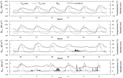
2.4. Climatic conditions
The climatic conditions during the measurement campaign are illustrated in Fig. 1, showing the trans-mitted net radiation, the top soil surface temperature, the air temperature at 7 m and rainfall. The 24 days of the data set, from 14 March to 6 April, can be split up in two periods. Up to 27 March sunny conditions are prevalent, except on 14 March (overcast) and ex-cept for some passing clouds in the mornings of 15, 16 and 24 March. From 28 March, conditions start to change. Clouds appear on 28 March. 29 March is overcast from 10 a.m. and large rainfall occurs dur-ing the followdur-ing night. On 30 March net radiation remains lower than 20 W m−2. After this first rain the weather remains unstable during the last 8 days. Most days are affected by passing clouds and rainfall fre-quently occurs. During the first period, the Bowen ra-tio is generally between 1 and 1.5. It remains around 1 during the 3 cloudy days (from 28 to 30 March) and drops to 0.5 or less from 31 March to the end of the experiment.
The period of measurement is also characterized by a large range of variation in air temperature. From 14 to 23 March, the weather is stable, with a repetitive daily cycle. Air temperature at 7 m varies between
maximum values of 14–17◦C around 3 p.m. and
min-imum values of 3–5◦C around 7 a.m. After a short
period of cooling on 24 and 25 March (maximum: 10–12◦C; minimum: −2−0◦C), air temperatures in-creases again to reach the maximum values for the whole period of measurement on 27 March
(maxi-mum: 22◦C; minimum: 12◦C). From 28 to 30 March,
nocturnal minimum values remain high (10–12◦C),
Fig. 1. Climatic conditions during the March–April 1998 experiment in the Landes forest.
3. Validation of eddy flux measurements
3.1. Energy balance closure
When many runs are lumped together and averaged, eddy fluxes measured above a forest appear gener-ally valid, as proved by the energy balance closure on a daily basis (Jarvis et al., 1997) or an hourly basis (Baldocchi and Vogel, 1997; Berbigier et al., 1998). Of course, at such short time scales this requires reli-able estimates of the storage terms in the soil (G) and in the different compartments of the canopy (J), over-storey, litter, trunks, and the air layer below the flux measurement level.
In the lower part of the canopy two problems arise. First, the eddy covariance method is subject to crit-icism because the underlying requirements are not always fulfilled: low wind speed, strong heterogene-ity and intermittent turbulence contribute to making the convergence of the statistical moments difficult. Second, the relative importance of the storage terms in the understorey energy balance is substantially
higher than in the previous case. At canopy scale in day-time conditions, the sum (F) of the sensible (H) and latent (LE) heat fluxes corresponds to about 90% of the incident net radiation, whereas at the under-storey level this proportion is on average only about 60% of the transmitted net radiation Rn,b, and can be
as low as 40%. Altogether, it is more difficult in these conditions to obtain a correct energy balance closure. As an example, Baldocchi and Vogel (1997) ob-tained a relatively poor closure over the understorey, whereas their results were rather good above the forest.
In Fig. 2, we plotted the sum of turbulent fluxes
(F = H+LE) measured above the forest floor
di-rectly against the transmitted net radiation Rn,b, for the
whole data set. Three main features can be seen: (i) for day-time data (Rn,b>0) there is a large discrepancy
between F and Rn,b(the slope of the linear regression
for day-time data is 0.63), (ii) there is a large scat-ter (r2is only 0.76 for day-time data), (iii) during the night F is about zero, whereas Rn,bis negative (down
Fig. 2. Sum of eddy fluxes (F) vs. net radiation (Rn,b), below the forest canopy. The straight line represents the linear regression for day-time data (Rn,b>0).
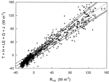
In Fig. 3, the sum of storage terms (S =G+J)
was added to the sum of turbulent fluxes. The sum of storage terms and turbulent fluxes,S+F, is noted
T. The residual difference between Rn,band T is
fur-ther noted R. The results are remarkable: the whole set of points is now centered around the 1:1 line. Table 1 shows that the slope of the regression line for the whole data set is 0.99, that the intercept is negligi-ble (0.49 W m−2) and that the scatter has substantially
decreased. In other words a careful evaluation of the various storage terms allow us to obtain a satisfac-tory closure of the energy balance. Incidentally, these results show that at night the turbulent fluxes at the understorey level are negligible, Rn,bbeing only
com-pensated by the storage terms. This is an important difference with what is currently observed above a forest canopy.
It must be mentioned that the ratio F/Rn,b varies
to a large extent (from about 0.4 to 0.8) during the
Table 1
Regressions of the sum of storage terms and eddy fluxes versus net radiation Rn,bestimated just above the understorey Whole data set Day-time data (Rn,b > 0) Regression not
forced through 0
Regression forced through 0
Regression not forced through 0
Regression forced through 0
Slope 0.99 0.99 0.97 0.99
intercept (W m−2) 0.49 0 1.96 0
r2 0.94 0.94 0.88 0.88
Fig. 3. Sum of eddy fluxes and storage terms (T) vs. net radiation (Rn,b), below the forest canopy. The slope of the linear regression for day-time data (not illustrated) is 0.99, withr2 =0.88 (see Table 1). The straight lines (other than 1:1) correspond to the selection thresholds defined in Section 3.3, using the “a” (slope) and “b” (intercept) coefficients. The two examples given here correspond to(a, b)=(0.1,10)and (0.15, 0), respectively.
experiment, in response to the evolution of climatic conditions. From 14 to 26 March, turbulent fluxes represent about 60% of the net radiation. From 27 to 31 March, they represent only 40 to 50% of Rn,b.
At the end of the experiment, from 1 to 6 April, they are largely dominant in the energy balance (70 to 80% of Rn,b). As mentioned above, this third period
corresponds to a strong decrease in Bowen ratio, the latent heat flux being twice or three times larger than the sensible heat flux. The ratio LE/Rn,b rises from
about 0.3 to 0.4–0.5, while the ratio H/Rn,b remains
unchanged. Of course, as for nocturnal data, this
evolution of the ratio F/Rn,b is compensated by an
equivalent evolution of the ratio S/Rn,b.
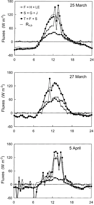
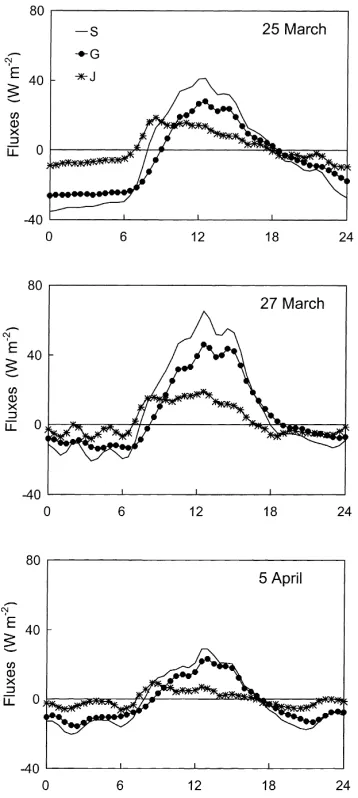
turbulent fluxes were found to be close to zero, the good closure of the energy balance at night is essen-tially a validation of the storage terms. Thus, day-time data give a better idea of the quality of the energy bal-ance closure from the point of view of the validation of turbulent fluxes. The regression coefficients remain high (0.88 over the whole period) and the slopes of the regressions are close to the previous values (0.97 or 0.99 when the intercept is forced through the origin). Fig. 4 shows 3 single days of the experiment, which correspond to the three periods just mentioned. The main features presented by net radiation are fairly well reproduced by the turbulent fluxes. The day-to-day variation of the ratio F/Rn,b is well compensated by
the variation of the storage terms. Whatever the rela-tive contributions of F and S, the energy balance clo-sure is correct (i.e. T =F +S ≈Rn,b), except for
occasional half-hourly values. At night, the sum of the storage terms is close to net radiation and follows its variations even at short time scales. This is particu-larly well illustrated before sunrise on 27 March and confirms that the near-zero values of the nocturnal tur-bulent fluxes, observed on Fig. 2, are real.
3.2. Variability of eddy flux measurements
Fig. 4 also shows that non-zero values of turbulent fluxes on 5 April before sunrise are not compensated by any concomitant variation in Rn,bor S. These peaks
result from errors in the measurement of latent heat fluxes due to the rain events illustrated in Fig. 1. Also, a few peaks in the time series of the eddy fluxes, not matching net radiation, appear during fine days (e.g. 25 March in the early afternoon, 27 March in the late morning).
Such occasional excursions, not validated by the energy balance, are not specific to the data recorded in the lower part of the forest, and have also been ob-served frequently on measurements performed above vegetation canopies (Lamaud et al., 1994; Blanken et al., 1997). It is indeed a common fact that turbulent flux measurements exhibit noticeable run-to-run vari-ability. This variability is sometimes compatible with the variation of net radiation due to passing clouds but it can also be observed in the absence of any perturbation in the diurnal evolution of Rn,b. Blanken
et al. (1997) noticed that a “saw-tooth” pattern is often observed in both H and LE, especially in clear
Fig. 4. Diurnal variation of net radiation (Rn,b), the sum of eddy fluxes (F), the total storage (S) and the sum of eddy fluxes and storage terms (T), below the forest canopy, for 25 and 27 March and 5 April 1998.
sky conditions when Rn,bvaries smoothly throughout
basis, the validity of turbulent flux measurements in the lower part of the forest canopy, Fig. 3 shows that the residual term of the energy balance (R= |Rn,b−
T|) is larger than 15% of Rn,bfor a large amount of
data. Only 40% of day-time data and 35% of nocturnal data are included in the area defined by the slopes 0.85–1.15. Depending on the intended use of the data set, a more or less severe selection should then be operated on the basis of the residue of the energy balance. This is the object of the next section.
3.3. Data selection
As mentioned in the introduction, ecophysiological and turbulence studies do not require the same de-gree of accuracy in eddy flux measurements. In the first case, we suggest to compare the residual term of the energy balance to net radiation, which amounts to expressing the selection threshold as a fraction of
Rn,b. In the second case, the selection threshold will
be expressed as a fraction of the sum of the turbulent fluxes, F.
3.3.1. Selection for ecophysiological studies
In ecophysiological studies it is necessary to keep a reasonable amount of data from night, early morning and late afternoon, even if the accuracy on both storage and eddy flux measurements is relatively low during these periods. Thus, the selection threshold should al-low a larger latitude for data at small positive Rn,b, as
well as for negative Rn,b. Indeed, Fig. 3 shows that a
selection threshold defined as a fraction of Rn,b(0.15
in this example) would reject many samples at low
Table 2
Fraction of selected data for various “a” and “b” coefficientsa Nocturnal data (Rn,b<0)
the 1:1 line. To avoid this we can define the rejection threshold as a linear function of Rn,bwith a non-zero
value of the intercept
R < a|Rn,b| +b
Fig. 3 shows two examples of selection thresholds using respectively the values (0.1, 10) and (0.15, 0) for the selection coefficients (a, b). While both approaches allow us to reject the most doubtful data, the first one preserves a reasonable amount of data at negative and small positive Rn,b, which is obviously not the case
for the second one.
Table 2 presents in a quantitative way the conse-quences of the selection with different (a, b) pairs. This table distinguishes three categories of data:
nocturnal data, day-time data with Rn,b less than
60 W m−2 and day-time data with Rn,b larger than
60 W m−2. Concerning day-time data, the fraction of selected data is of the same order for Rn,bhigher or
lower than 60 W m−2, provided that b is not zero. This gives a fairly good description of the daily and day-to-day evolution of turbulent fluxes, as illustrated
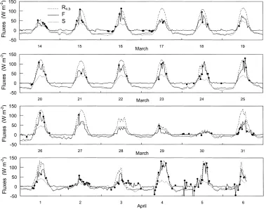
in Fig. 5 with (a, b) = (0.1,10). Indeed, the most
spurious data are rejected, while the main tendencies in the evolution of the turbulent fluxes are preserved. A comment must be made concerning nocturnal data. It was noticed in Section 3.1 that the near-zero values of nocturnal turbulent fluxes were validated by the mean energy balance closure. In other words, the nocturnal
energy balance can be written as Rn,b ≈ S.
Fig. 5. Times series of net radiation (Rn,b), the total storage (S) and the sum of eddy fluxes (F), below the forest canopy, for the period from 14 March to 7 April 1998. Filled circles represent the values of F rejected witha=0.1 andb=10.
selecting nocturnal eddy flux data, except for the case of strongly spurious values like on 5 April during rain events. For illustrative purpose, the nocturnal data pre-sented in Table 2 give an idea of the quality of the storage estimates, but this point will not be further discussed in this paper dedicated to the validation of eddy flux measurements.
3.3.2. Selection for turbulence studies
If the data set is to be used for specific analyses of turbulent transfer, a data selection like that illustrated in Fig. 5 is clearly not adequate. Indeed, the relative uncertainty on the values of the eddy fluxes is much
too high. For example, with (a, b) = (0.1,10), the
absolute uncertainty is 16 W m−2 when Rn,b equals
60 W m−2. As eddy fluxes were found to represent
only about 60% of Rn,b (see Section 3.1), the
rela-tive uncertainty represents in this case nearly 50% of the value of F. Furthermore, this relative uncertainty
increases for lower values of Rn,b. For this second kind
of studies, we suggest using a selection criterion based on the ratio of the energy balance residue to the sum of the turbulent fluxes themselves, i.e.
R < α|F| or R′= R
|F| < α
Table 3 shows how the current data set is qualified us-ing this criterion with different values ofα. The qua-lity of the eddy flux measurements may seem poor as, for example, only 53% of the data corresponding to
Rn,bhigher than 60 W m−2and 16% of data from the
Table 3
Fraction of selected data for various thresholds of the relative residueR′=R/|F|(see Section 3.3.2)a
R′ <50% R′ <40% R′ <30% R′ <20% R′<10%
Day-time data with Rn,b> 60 W m−2 (%) 88 (89) 82 (86) 72 (76) 53 (59) 34 (38) Day-time data with Rn,b<60 W m−2(%) 42 (48) 33 (40) 24 (30) 16 (22) 9 (15)
aThe values within brackets refer to the clear days (120 samples forR
n,b>60 W m−2, 88 samples forRn,b<60 W m−2) and the others to the whole data set (199 samples and 259 samples, respectively).
degree of confidence, this type of selection is more adapted, even if the data set is to be considerably reduced. Furthermore, it must be noted that a large part of the data rejected with this criterion come from overcast (for instance 2 April where Rn,bis less than
60 W m−2for the whole day) or partially cloudy days
like 5 April. In the latter case, because of the vari-ability in both Rn,b and F, it is more difficult to get
a good energy balance closure on a run-to-run ba-sis. As presented in Table 3, the fraction of selected data increases appreciably when only clear days are considered, which corresponds to about 50% of our current data set. A characterization of turbulent trans-fer in the lower part of the forest canopy, based on a spectral or statistical analysis of turbulent variables, should only be performed, at least in a first step, on this data subset.
4. Modelling the storage terms
Measuring the storage terms G and J involves a very constraining experimental procedure, which is not feasible in all field experimentations. However, the selection methodology described above should still be applicable if the storage terms could be properly estimated from simple meteorological parameters. For instance Diawara et al. (1991) showed that the total storage at canopy scale could be approximated by a linear function of the rate of change in air temperature above the forest. Ogée et al. (2000) concluded that
G can be expressed as a function of transmitted net
radiation, with a time lag of half an hour, and the temperature difference between the litter surface and the air just above it (20 cm). The object of this section is to suggest a simple model for the storage terms, that could be used if no proper measurements were available.
4.1. Daily variations of the storage terms in the soil and the canopy
Examples of the variation in G, J and the total
stor-age,S =G+J, are shown in Fig. 6 for the same 3
days as in Fig. 4. To reduce the variability of the var-ious storage terms, the raw data were smoothed over three points with coefficients 0.25, 0.5 and 0.25. Soil storage G appears predominant for most of the day and during the night, but canopy storage also plays a significant role, especially during the transition period around sunrise. In order to understand the behavior of the various terms Fig. 7 shows the contribution of the four components (Jh, Jl, Jtand Jw) to the storage J in
the canopy layer up tozr =6 m.
Latent heat storage Jwdoes not exhibit any clear
ten-dency and always remains between 3 and−3 W m−2. Although its relative contribution to J is larger during the period from 1 to 6 April it always remains negli-gible relative to the total storage S. Jw will therefore
not be taken into account in the model.
Both Jhand Jlhave a significant contribution in the
early part of the day. They both decrease along the day and become negative around 3 to 4 p.m. They remain negligible relative to G for most of the afternoon. Their specific form of variation is responsible for the appar-ent time lag between the soil storage term G and total storage S. Thus, if heat storage in the canopy air space and the litter is not taken into account in the energy balance, it will not only lead to an underestimation of the sum of storage and turbulent fluxes (T =F +S), but also to a systematical bias introducing a non-linear relation between T and Rn,b. Given the similarity in
the time variation of Jhand Jl, we will only consider
their sumJ∗=Jh+Jl.
Heat storage in the trunks between 0 and 6 m, Jt,
Fig. 6. Diurnal variation of soil storage (G), canopy storage up to 6 m (J) and total storage (S=G+J) for 25 and 27 March and 5 April 1998.
represents about 5% of the transmitted net radiation on 25 and 27 March, as for the whole period from 14 to 31 March. Jt is always strongly correlated to the soil
storage G, but with a time lag of about 2 h. Like G, it decreases during the last period of the experiment when the ratio F/Rn,breaches 0.7–0.8, because of the
increase in LE. Because of this correlation between the storage in trunks and soil, Jt will not be modelled
as part of J but as an additive term to the soil storage
G. This introduces an equivalent soil storage (G∗ =
Fig. 7. Diurnal variation of the various components of canopy storage up to 6 m (J) for 25 and 27 March and 5 April 1998: latent heat storage (Jw), sensible heat storage in air (Jh), litter (Jl) and trunks (Jt).
Jt+G) which is only slightly larger than G (Fig. 8).
As Jt is low compared to G, the systematical error
induced by the time lag between those two terms has no consequence on the energy balance closure.
4.2. Modelling the storage terms G∗and J∗ from experimental values
Fig. 8. Sum (G∗) of soil storage (G) and trunk storage up to 6 m
(Jt) vs. G.
parameterized as a function of dT7m/dt (following
Diawara et al., 1991 who estimated the total heat stor-age from the rate of change in air temperature above the forest canopy). The linear regression between J∗ and dT7m/dt was performed over the whole data set.
The result is
J∗=4.2dT7m
dt
The statistics are given in Table 4 and this modelled
J∗is plotted in Fig. 9 versus the experimental values of J∗. The regression between J∗and dT7m/dt is quite
good (r2=0.93) even if the relation is not perfectly linear. This is primarily due to the impact of Jlwhich
is less correlated to dT7m/dt than Jh.
Regarding the storage in the soil and the trunks, we can apply the method described in Ogée et al. (2000) to the current data set, using the equivalent storage term G∗instead of the soil storage term G. The linear regression provides
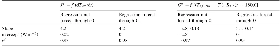
Table 4
Main statistics for the parameterization of J∗(sum of sensible heat storage in litter and canopy air space) and G∗(sum of heat storage in
soil and trunks)
J∗=f (dT
7m/dt) G∗=f [(Ta,0.2m −Tl), Rn,b(t−1800)] Regression not
forced through 0
Regression forced through 0
Regression not forced through 0
Regression forced through 0
Slope 4.2 4.2 2.8, 0.18 3.1, 0.14
intercept (W m−2) 0.02 0 −2.8 0
r2 0.93 0.93 0.97 0.95
Fig. 9. Comparison between the modelled and the experimental terms for the sum of heat storage in the canopy air space up to 6 m and the litter (J∗).
G∗=2.8(Ta,0.2m−Tl)+0.18Rn,b(t−1800)−2.8
where (Ta,0.2m−Tl) is the temperature difference
be-tween the litter surface and the air just above it (20 cm) and Rn,b(t−1800) is the transmitted net radiation with
a time lag of half an hour.
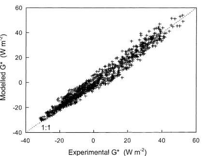
The statistics for the regression are also given in Table 4 and the results are plotted in Fig. 10. Even if the intercept is small (−2.8 W m−2), the slopes differ
Fig. 10. Comparison between the modelled and the experimental terms for the sum of heat storage in the soil and the trunks up to 6 m (G∗).
4.3. Estimation of storage terms from the energy balance closure
It is now possible to suggest a method for estimat-ing the storage terms when no proper measurements are available, which is a common situation given the number of sensors required for such an estimation. The method is based on the results obtained above: storage terms can be expressed as a linear combina-tion of dT7m/dt, [Ta,0.2m−Tl)] and Rn,b(t−1800), and
the various coefficients are calculated empirically by a multiple linear regression of the residual term of the energy balanceRn,b−H−LE over these three
param-eters. Doing this, the following functions were found
J∗′ =5.4dT7m
dt
G∗′ =2.5(Ta,0.2m−Tl)+0.18Rn,b(t−1800)−3.1
where J∗′and G∗′are the estimated values of J∗and
G∗. Despite the variability of the termR
n,b−H−LE,
resulting from occasional errors in turbulent flux mea-surements, the coefficient of the regression is accept-able (0.78). The method provides a satisfactory esti-mate of the storage terms, as can be seen from Fig. 11 showing the half-hourly variations of estimated and measured storage terms for the 3 days of Figs. 4, 6 and 7. The question now arises as to whether the small dif-ferences between estimated and experimental values
Fig. 11. Diurnal variation of the experimental storage terms (G∗
and J∗) and the storage terms estimated from the residual of the
energy budget (G∗′and J∗′), for 25 and 27 March and 5 April
1998. The estimated storage terms are both represented by solid lines.
have significant consequences on the energy balance closure and the selection of eddy fluxes.
4.4. Consequences of storage estimation on the energy balance closure
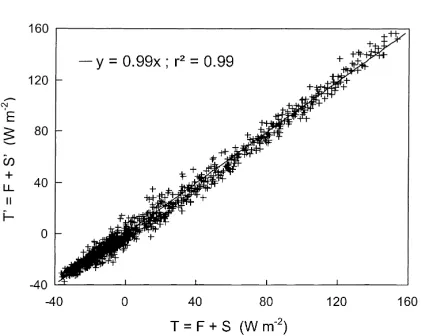
Fig. 12 provides a comparison ofT (=F +S)and
mea-Fig. 12. Comparison of the sum of eddy fluxes and storage terms computed with estimated (T′=F+S′) and experimental
(T =F+S) values for the storage terms.
sured (S = G+J) and estimated (S′ = G∗′ +J∗′) sums of storage terms. The agreement between T and
T′ is excellent, not only because the slope is close to 1, but above all because the scatter is small. Indeed, the difference between T and T′is most often less than 10 W m−2, in absolute value. If we compare this graph to Fig. 3, it is clear that the accuracy of the storage es-timation is good enough to allow a reliable selection of the data.
As an example, Table 5 presents the level of agree-ment between the data selections achieved using S or
S′, for different values of the “a” and “b” coefficients.
Table 5
The agreement in rejecting or selecting data using methods in-volving either S or S′ (see Section 4.4)a
Day-time data with Rn,b < 60 W m−2 (%)
Day-time data with Rn,b > 60 W m−2 (%)
a=0.15, b=10 89 95
a=0.1, b=10 88 93
a=0.05, b=10 86 92
a=0.15, b=5 76 95
a=0.1, b=5 71 92
a=0.05, b=5 66 82
a=0.15, b=0 69 90
a=0.1, b=0 72 85
a=0.05, b=0 82 83
aThe complement to 100% represents data selected by one method and rejected by the other.
Fig. 13. Sum of eddy fluxes (F) vs. net radiation (Rn,b), below the forest canopy, after data selection using measured (S) or estimated (S′) storage terms. The straight line (slope=0.63) is the linear
regression line displayed in Fig. 2.
For reasons explained in Section 3.3.1, only day-time data are presented, with the same categories as in Table 2. For the category corresponding to Rn,blarger
than 60 W m−2, the two methods are in agreement for a large subset of data (more than 80% for all (a, b) pairs). The agreement is not as good for Rn,b lower
than 60 W m−2but it remains acceptable (higher than 80%) if b equals 10.
Fig. 13 illustrates in a more explicit way the conse-quences of storage estimation on the selection of eddy flux measurements. Data were selected using S′or S, with the same coefficients as in Fig. 5 (i.e.a =0.1
andb =10) and plotted as H +LE versus Rn,b. A
comparison of this graph with Fig. 2 shows the benefit of the data selection. Whether estimated or measured storage terms are used, the scatter observed in the raw data is reduced, a large amount of spurious data being rejected likewise by the two methods.
5. Concluding remarks
canopy. Despite the particular conditions prevailing in this region, the eddy covariance method proved to be as reliable as for measurements performed over a bare soil, a short crop or a forest. This achievement was obtained at the expense of extensive measurements of all storage terms.
The methodology presented here was originally designed to extract reliable flux values from a contin-uous data set, for our own ecophysiological as well as turbulence studies. In the latter case in particular the demand in terms of accuracy is quite strong and an objective, automatic method had to be developed for selecting the best possible data. We also have an-other data set of great potential use from a different forest site in which no storage measurements were performed. This is actually a general case in contin-uous flux measurement campaigns, since measuring all storage terms represents a heavy experimental procedure. In order to perform eddy flux data se-lection we had to develop a method for estimating the storage term. As our method proved to be suc-cessful we consider that it may be of interest for other research groups involved in this type of field campaigns.
As described above, the method simply consists in estimating the storage terms from the mean energy bal-ance of the understorey. The total storage is expressed as a linear combination of three parameters (the rate of air temperature change under the canopy, the trans-mitted net radiation and the difference of temperature between the litter surface and the air just above), using empirical coefficients deduced from the mean energy balance closure. We showed that the parameterization of the storage terms was in good agreement with the experimental data, and that the effects of the data se-lection were generally similar whether experimental or estimated values were used. The effect of various selection criteria was also illustrated, giving rules for further work on such data sets.
List of symbols
a, b coefficients for the data selection based
on the residual difference R
Cp air specific heat (J kg−1K−1)
Cvi specific heat of component i of the
vegetation (J kg−1K−1)
e vapor pressure (Pa)
F sum of sensible heat flux H and latent
heat flux LE (W m−2)
G soil heat flux (W m−2)
G∗ sum of soil storage G and storage in the
trunks Jt (W m−2)
G∗′ estimated value of G∗from the residual
of the energy budgetRn,b−H−LE
(W m−2)
J heat storage in the forest layer below
the level of turbulent measurements zr
(W m−2)
Jh sensible heat storage in the canopy air
space up to zr (W m−2)
Jl sensible heat storage in the litter
(W m−2)
Jp energy fixed by photosynthesis (W m−2)
Jt sensible heat storage in the trunks
up to zr (W m−2)
Jv sensible heat storage in the vegetation
up to zr (W m−2)
Jw latent heat storage in the canopy air
space up to zr (W m−2)
J∗ sum of sensible heat storage in the litter
Jl and the canopy air space Jh(W m−2)
J∗′ estimated value of J∗from the residual
of the energy budgetRn,b−H−LE
(W m−2)
Lp specific energy equivalent of CO2
fixation (J kg−1)
R absolute value of the residual difference
between Rn,band T (R= |Rn,b−T|)
(W m−2)
R′ residual difference between R
n,band T,
expressed as a fraction of F (R′=R/|F|)
Rn,b net radiation estimated just above the
understorey (W m−2)
Rn,b
(t−1800) net radiation above the understorey, with a time lag of half an hour (W m−2)
S sum of storage terms G and J (W m−2)
S′ sum of estimated storage terms G∗′and
J∗′(W m−2)
t time (s)
T sum of turbulent fluxes and measured
T′ sum of turbulent fluxes and estimated storage terms (W m−2)
dT7m/dt rate of change in air temperature at
7 m above the understorey (◦C s−1)
Ta air temperature (◦C)
Ta,0.2m air temperature at 20 cm (◦C)
Tl temperature at the top of the litter
(◦C)
Tvi temperature of component i of the
vegetation (◦C)
z altitude, counted positive away from the
soil surface (m)
zr level of turbulent measurements
(6 m)
Greek letters
α coefficient for the data selection based
on the residual difference R′
Γ psychrometric constant (≈66 Pa K−1)
ρ air density (kg m−3)
ρvi density of component i of the vegetation
(kg m−3)
Acknowledgements
Part of the data used in this paper was collected during the EUROFLUX project supported by the European commission (Programme environment and climate, contract ENV4-CT95-0078). The authors are indebted to J.M. Bonnefond, M.R. Irvine, A. Kruszewski and P. Mellmann for their contribution to the data collection and processing.
References
Aubinet, M., Grelle, A., Ibrom, A., Rannik, Ü., Moncrieff, J., Foken, T., Kowalski, A.S., Martin, P.H., Berbigier, P., Bernhofer, Ch., Clement, R., Elbers, J., Granier, A., Grünwald, T., Morgensten, K., Pilegaard, K., Rebmann, C., Snijders, W., Valentini, R., Vesala, T., 1999. Estimates of the annual net carbon and water exchange of European forests: the EUROFLUX methodology. Adv. Ecol. Res. 30, 113–175. Baldocchi, D.D., Vogel, C.A., 1997. Seasonal variation of energy
and water vapor exchange rates above and below a boreal jack pine forest canopy. J. Geophys. Res. 102 (D24), 28939– 28951.
Baldocchi, D.D., Vogel, C.A., 1996. A comparative study of water vapor, energy and CO2flux densities above and below a
temperate broadleaf and a boreal pine forest. Tree Physiol. 16, 5–16.
Berbigier, P., Bonnefond, J.M., 1995. Measurement and modeling of radiation transmission within a stand of maritime pine (Pinus pinaster Ait.). Ann. Sci. For. 52, 23–42.
Berbigier, P., Ogée, J., Bonnefond, J.M., Lamaud, E., Brunet, Y., 1998. Mass and energy fluxes over a pine forest canopy: energy and water balance closure, and intra-annual variations in water and radiation use efficiencies. In: 23rd EGS General Assembly, Nice, 20–24 April 1998. News Letter, European Geophysical Society, poster OA247, p. 177.
Blanken, P.D., Black, T.A., Yang, P.C., Neumann, H.H., Nesic, Z., Staebler, R., den Hartog, G., Novak, M.D., Lee, X., 1997. Energy balance and canopy conductance of a boreal aspen forest: partitioning overstory and understory components. J. Geophys. Res. 102 (D24), 28915–28927.
Carrara, A., Lamaud, E., Lopez, A., Brunet, Y., 2000. Ozone dry deposition measurements above and within a maritime pine (Pinus pinaster Ait.) forest. Atmos. Env., submitted for publication.
Coe, H., Gallagher, M.W., Choularton, T.W., Dore, C., 1995. Canopy scale measurements of stomatal and cuticular O3uptake by sitka spruce. Atmos. Env. 29, 1413–1424.
Diawara, A., Loustau, D., Berbigier, P., 1991. Comparison of two methods for estimating the evaporation of a Pinus pinaster (Ait.) stand: sap flow and energy balance with sensible heat flux measurements by an eddy covariance method. Agric. For. Meteorol. 54, 49–66.
Grace, J., Lloyd, J., McIntyre, J., Miranda, A.C., Meir, P., Miranda, H.S., Moncrieff, J.M., Massheder, J., Wright, I.R., Gash, J., 1995. Fluxes of carbon dioxide and water vapor over an undisturbed tropical rain forest in south-west Amazonia. Global Change Biol. 1, 1–12.
Grace, J., Malhi, Y., Lloyd, J., McIntyre, J., Miranda, A.C., Meir, P., Miranda, H.S., 1996. The use of eddy covariance to infer the net carbon dioxide uptake of Brazilian rain forest. Global Change Biol. 2, 209–218.
Jarvis, P.G., Massheder, J.M., Hale, S.E., Moncrieff, J.B., Rayment, M., Scott, S.L., 1997. Seasonal variation of carbon dioxide, water vapor, and energy exchanges of a boreal black spruce forest. J. Geophys. Res. 102 (D24), 28953– 28966.
Lamaud, E., Brunet, Y., Berbigier, P., 1996. Radiation and water use efficiencies of two coniferous forest canopies. Phys. Chem. Earth 21, 361–365.
Lamaud, E., Brunet, Y., Labatut, A., Lopez, A., Fontan, J., Druilhet, A., 1994. The LANDES experiment. Biosphere–atmosphere exchanges of ozone and aerosol particles above a pine forest. J. Geophys. Res. 99 (D8), 16511–16521.
Loustau, D., Cochard, H., 1991. Utilisation d’une chambre de transpiration portable pour l’estimation de l’évapotranspiration d’un sous-bois de pin maritime à molinie (Molinia coerulea (L.) Moench). Ann. Sci. For. 48, 29–45.
Moncrieff, J.B., Massheder, J.M., de Bruin, H., Elbers, J., Friborg, T., Heusinkveld, B., Kabat, P., Scott, S., Soegaard, H., Verhef, A., 1997. A system to measure surface fluxes of momentum, sensible heat, water vapor and carbon dioxide. J. Hydrol. 188/189, 589–611.
Munger, J.W., Wofsy, S.C., Bakwin, P.S., Fan, S.M., Goulden, M.L., Daube, B.C., Goldstein, A.H., Moore, K.E., Fitzjarrald, D.R., 1996. Atmospheric deposition of reactive nitrogen oxides and ozone in a temperate deciduous forest and a subarctic
woodland. 1. Measurements and mechanisms. J. Geophys. Res. 101 (D7), 12639–12657.
Ogée, J., Lamaud, E., Brunet, Y., Berbigier, P., Bonnefond, J.M., 2000. A long-term study of soil heat flux under a forest canopy. Agric. For. Meteorol. 106, 173–187.