CORRECTION OF AIRBORNE PUSHBROOM IMAGES ORIENTATION USING BUNDLE
ADJUSTMENT OF FRAME IMAGES
K. Barbieuxa, D. Constantina, B. Merminoda. a
Geodetic Engineering Laboratory, ´Ecole Polytechnique F´ed´erale de Lausanne, Lausanne, Switzerland [email protected], [email protected], [email protected]
ICWG III/I
KEY WORDS:Hyperspectral, Georeferencing, Geometric Correction, Pushbroom, Bundle Adjustment.
ABSTRACT:
To compute hyperspectral orthophotos of an area, one may proceed like for standard RGB orthophotos : equip an aircraft or a drone with the appropriate camera, a GPS and an Inertial Measurement Unit (IMU). The position and attitude data from the navigation sensors, together with the collected images, can be input to a bundle adjustment which refines the estimation of the parameters and allows to create 3D models or orthophotos of the scene. But most of the hyperspectral cameras are pushbrooms sensors : they acquire lines of pixels. The bundle adjustment identifies tie points (using their 2D neighbourhoods) between different images to stitch them together. This is impossible when the input images are lines. To get around this problem, we propose a method that can be used when both a frame RGB camera and a hyperspectral pushbroom camera are used during the same flight. We first use the bundle adjustment theory to obtain corrected navigation parameters for the RGB camera. Then, assuming a small boresight between the RGB camera and the navigation sensors, we can estimate this boresight as well as the corrected position and attitude parameters for the navigation sensors. Finally, supposing that the boresight between these sensors and the pushbroom camera is constant during the flight, we can retrieve it by matching manually corresponding pairs of points between the current projection and a reference. Comparison between the direct georeferencing and the georeferencing with our method on three flights performed during the Leman-Baikal project shows great improvement of the ground accuracy.
1. CURRENT METHODS FOR PUSHBROOM DATA REGISTRATION
1.1 Pushbroom Sensors
Pushbroom sensors are common to acquire hyperspectral data as they usually propose high spatial resolution and a high number of bands. They work as line sensors, and they are usually used on moving platforms to scan zones (see Figure 1).
optical center
x y
z
Figure 1. Pushbroom sensors are optical sensors consisting in a line of pixels. They are usually moved orthogonally to the line to construct images.
To establish a hyperspectral cartography of an area of interest, it is possible to mount such a sensor on an aerial vehicle and scan the area by flying over it. Each of the acquired hyperspectral lines has six orientation parameters, called Exterior Orientation Param-eters (EOP): three coordinates representing its position, and three angles representing its attitude. These parameters are relative to
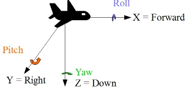
a coordinate system; in the following, we work with the WGS84 Geoid. The position parameters we use are latitude, longitude and altitude, and the attitude parameters are roll, pitch and yaw angles, defined as in Figure 2.
Figure 2. roll, pitch and yaw angles are rotation angles relative to the axis of the body frame.
Inherent parameters of the camera, called Interior Orientation Pa-rameters (IOP) also impact the georeferencing task: the focal length of the camera, its principal point location and the radial distortion of its lens. When all the orientation parameters are known for a single line, this line can be georeferenced.
1.2 Georeferencing
3 shows a projection of hyperspectral data where the navigation data used is obtained by integrating the information provided by the GPS+IMU system Ekinox-N designed by SBG Systems.
Figure 3. projection of hyperspectral data acquired while flying over EPFL (Lausanne, Switzerland), visualised in our software HypOS.
For a single flight line, trajectory models using random processes allow to achieve better ground precision (see (Lee and Bethel, 2001)), but in the general case, post-processing, using Ground Control Points (GCP) or extra information, is needed to compute a coherent and well georeferenced image. This is called Indirect Georeferencing. The GCP approach consists in matching points in our data with coordinates in the reference (i.e, on the Earth when these points have been measured on the field) and then ap-plying corrections to the navigation data according to this match-ing. In the case of a pushbroom sensor, one would need 3 GCPs per line to determine the 6 orientation parameters of a given line (see (Lee et al., 2000)), which is not feasible. But combining the direct and the indirect approach allows good georeferencing: a few GCPs can help to geometrically correct data after a first raw projection, using interpolation methods like Particle Swarm Op-timization (see (Reguera-Salgado and Mart´ın-Herrero, 2012)).
2. OUR APPROACH
In this section, our approach is detailed. It is decomposed as fol-lows: we perform a bundle adjustment of the RGB images cap-tured by our RGB camera during the flight. It utilizes the naviga-tion data output by integrating the GPS/IMU informanaviga-tion. Then, the corrected navigation data for the RGB camera is retrieved, and used to estimate the boresight between this camera and the IMU, as well as the corrected navigation data for the IMU, using a least-square compensation. The last step consists in projecting the hy-perspectral data using this new navigation data and performing a last correction, taking into account the boresight between the pushbroom sensor and the IMU; this boresight is estimated using tie points between the latest projection and the reference. Figure 4 summarizes this process.
2.1 Bundle Adjustment of RGB Images
Using feature matching techniques, RGB images can be stitched together to create a 3D model of the area. If a priori navigation data is also given, the process can correct it as well as the IOP like the focal length of the camera, the position of its principal point and the radial distortion. This process is called bundle ad-justment (see (Triggs et al., 2000) for reference). In our case, we use the navigation data integrated by the Kalman filter. Even though it is different from the navigation data for the RGB cam-era (since there is a boresight and a lever-arm between the two),
Figure 4. flowgram of our approach.
it is still close enough to be considered as a good first estimation of the orientation parameters of the camera. The bundle adjust-ment is processed using Agisoft PhotoScan (see (Agisoft, 2013)); Figure 5 shows a 3D model of ´Ecole Polytechnique F´ed´erale de Lausanne (EPFL) produced by this software.
Figure 5. digital elevation model with texture, created using Ag-isoft PhotoScan with our RGB and navigation data.
From there, we can retrieve corrected navigation data for the RGB camera.
2.2 Navigation Sensors Data Correction
The orientation parameters output by the previous step are for the frame camera. The correct parameters for navigation sensors are not the same, since there is a lever-arm as well as a boresight between them and the camera. Since our hyperspectral camera has a frequency 50 times higher than the one of our RGB camera, only one pushbroom line out of 50 can be directly corrected; we need to use the data acquired by navigation sensors to interpolate between the corrections.
a consequence, navigation sensors data can be used as such to interpolate between the corrections of the camera position.
Consider a position parameter p among latitude, longitude and altitude. Letprandpcbe respectively the raw value of this parameter (output of the Kalman Filter) and the corrected value. Lett0be the timestamp of a line corrected thanks to the bundle
adjustment. So is the line which timestamp ist0+ 50∆t, where
∆tis the sampling time of the hyperspectral camera. Since the IMU is a drifting sensor (accurate for short periods of time, but getting less and less accurate as time goes by), the variations it gives aroundt0 are highly reliable close tot0, and less when
getting closer tot0+ 50∆t. Same goes for the variations around
t0+ 50∆t. We therefore interpolatepc, fort∈[t0, t0+ 50∆t],
λ(t) is the weight given to the navigation data close tot0. Its
value is given by Equation 2.
λ(t) =t0+ 50∆t−t
50∆t (2)
2.2.2 Attitude Correction The attitude of the navigation sen-sors has to be computed. Indeed, to interpolate the attitude data, it is not possible to use the data from the navigation sensors as such, since it refers to its own frame, while the attitude given by the bundle adjustement refers to the RGB camera frame. At a given location, letRCamera
N ED be the rotation matrix from the North-East-Down local-level frame to the camera frame,RIM UN ED the one from the local-level frame to the IMU and Rbore = RCamera
IM U the rotation representing the boresight from the IMU to the camera. The relation between these matrices is given by Equation 3.
RboreRIM UN ED=R Camera
N ED (3)
Each of these rotation operators can be characterised by its roll, its pitch and its yaw, applied in this order: roll rotation around the x-axis, pitch rotation around the y-axis, and yaw rotation around the z-axis. Letr, p, ybe these 3 parameters; the corresponding rotation operator is given by Equation 4.
R(r, p, y) =
This boresight is constant during the flight as the sensors are rigidly attached to the vehicle. We call (rb, pb, yb) its roll, pitch and yaw. Similarly, at time t, let(rn(t), pn(t), yn(t))be the orientation parameters output by the navigation sensors, and (rc(t), pc(t), yc(t))the one for the RGB camera (given by the bundle adjustment). Let k be the number of RGB images avail-able, and(ti), i∈[1, k]the times of acquisition of each image.
The drifts (errors) in the orientation parameters added to the cur-rent drifts at time ti are called(dri, dpi, dyi). For each time ti, i∈[1, k], we can rewrite Equation 3 using the orientation pa-rameters of each rotation matrix. The set of equations obtained is given by 5.
and the subsequent noise from gyrometers have been added. Therefore, this model allows to keep the time-dependency of the drifts while having parameters that shall be small. Boresight pa-rameters shall also have low values, as the sensors are rigidly attached, pointing in the same direction, in our system. By re-trieving the orientation parameters from the left-hand side and the right-hand side of each equation in 5, we get a set of3k equa-tions with3k+ 3unknown parameters (all the drifts plus the 3 parameters of the boresight). This can be seen as an optimization problem: consider the vector of all the parameters to be deter-mined, as given by Equation 6.
v=
under the constraints given by the set of equations 5. With all parameters equal to 0, the equations are not verified, and for each equation there is a gap between the left-hand side and the right-left-hand side. If we callwthe column vector which elements are all these gaps andB the Jacobian matrix of the set, then it is known, using Lagrange multipliers theory, that vcan be approximated by Equation 7.
v=BT(BBT)−1w (7)
(the boresight). The rest of the corrected navigation sensors data is interpolated using the exact same interpolation method as de-scribed in 2.2.1.
2.3 Pushbroom Camera Attitude Correction
Once the attitude from the navigation sensors is known, the last step is to find the boresight between them and the pushbroom camera. A georeferenced RGB orthophoto and a georeferenced digital elevation model can be imported from Agisoft PhotoScan to our software HypOS, based on the NASA Worldwind SDK; overlooking at this unknown boresight, a first projection of the hyperspectral data can be made. Then, we manually point at cor-responding pairs of points between the RGB data and the hyper-spectral data. This is possible as the hyperhyper-spectral data can be seen as RGB, using 3 bands of the spectrum roughly correspond-ing to red, green and blue. With a large enough set of pairs, it is then possible to find the best boresight, as well as some IOP (focal length, principal point coordinates), to match these pairs. In the Earth-centered Earth-fixed frame, consider P P = (xpp, ypp, zpp)as the principal point of the pushbroom camera, andG= (xG, yG, zG)as a ground point we want to match; let (r, p, y)be the three orientation parameters of the boresight from the IMU to the camera. In the front-right-down frame of the cam-era centered at the principal point, the coordinates of a pixel are (δx, ypix+δy, f+δf)whereypixis the coordinate of the pixel along the line of the pushbroom andfis our input estimation of the focal length. If the principal point was centered relatively to the camera,δxandδy would be zero; but it is not rigourously true, thereforeδxandδyare interior orientation parameters that we might want to determine accurately.
For a given pair, Equation 8, also known as the collinearity equa-tion, should be verified.
6 unknown parameters have to be determined. This is possi-ble as long as 6 pairs of points are input. Then, these param-eters can be determined by a least-squares approximation. Let k be the number of input pairs, (Fi), i ∈ [1, k] the k corre-sponding functions as described in Equation 8,vthe vector of the six parameters to be found, andw the vector of the gaps (Fi(0,0,0,0,0,0)), i ∈ [1, k]. The estimation of the parame-ters can be refined using Equation 9.
δv= (ATA)−1AT(−w) (9)
This compensation can be applied iteratively till the correction is smaller than a given threshold. The output includes the boresight and the correction of interior orientation parameters; with these, navigation data for the pushbroom sensor is computed, and then we can georeference the data.
3. RESULTS
To assess the performance of our method, we compare here the precision of the projection before and after using it, on 3 flights of different mean elevations. These flights were performed in the
context of the Leman-Baikal project, which consists in a study of both lake Geneva (Switzerland) and lake Baikal (Russia) by making aerial surveys with hyperspectral cameras (see (Akhtman et al., 2014)). The cameras, together with the navigation sensors, are mounted on a ultralight trike. We have observed an important yaw drift along our flights, as well as a boresight, which resulted in bad georeferencing of the data. Therefore, this data is a good case study for our algorithm.
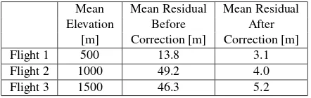
Our reference can either be the orthorectified photo output by PhotoScan or Bing Maps Imagery. The quality of each projection is characterized by its mean residual over a set of 50 reference ground control points. This has been tested on flights of different mean elevations. Results are summarized in Table 1.
Mean Mean Residual Mean Residual
Elevation Before After
[m] Correction [m] Correction [m]
Flight 1 500 13.8 3.1
Flight 2 1000 49.2 4.0
Flight 3 1500 46.3 5.2
Table 1. comparison of mean residual before and after correction for three flights of different altitudes.
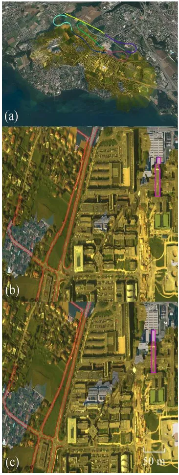
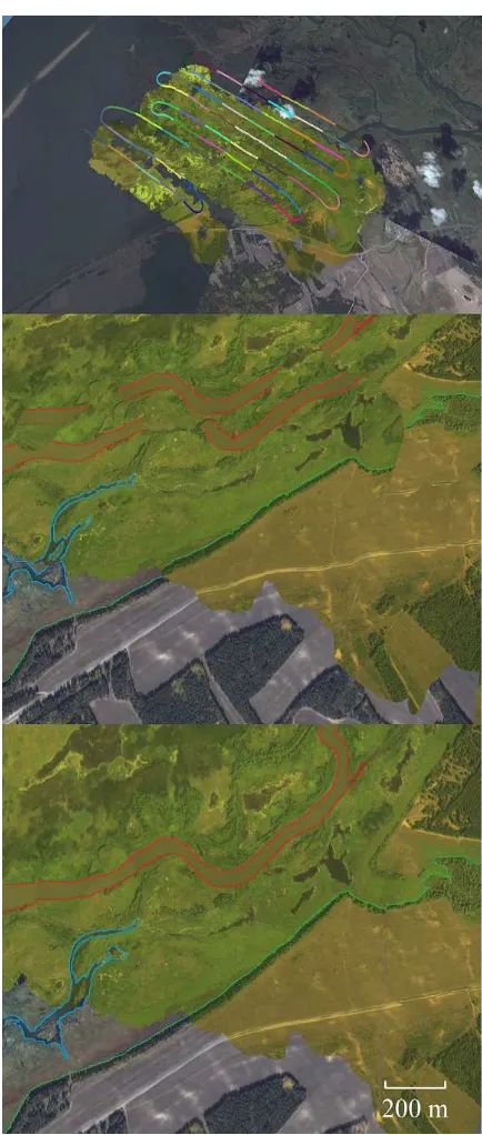
Quantitatively, images produced using our algorithm are much better georeferenced than the one created using Direct Georef-erencing. The correction gets more important with the altitude: for flights with a higher elevation, the mean residual using Direct Georeferencing grows up to 50 meters, while the impact of the height is way less important with our method. The Ground Sam-pling Distance (GSD) of our system is roughly a thousandth of the height. Consequently, the order of the residual is 1-6 GSD for the lower altitude flight, and 1-4 GSD for the other two. Qualitatively, Figures 6, 7 and 8 show, for each of these flights, the flight path, the raw projection (before correction) and the pro-jection after correction. The projected data is displayed with a lighter color to differentiate it from the reference (from Bing Maps Imagery) in the background. Particular features - roads, buildings or rivers - are highlighted in specific colors. They show that some shifts or distortions (due to misprojected overlapping lines) have been corrected in the processed images, which fit much better the background reference images and are more co-herent.
4. CONCLUSION
REFERENCES
Agisoft, L., 2013. Agisoft photoscan user manual. professional edition, version 0.9. 0.
Akhtman, Y., Constantin, D., Rehak, M., Nouchi, V. M., Bouf-fard, D., Pasche, N., Shinkareva, G., Chalov, S., Lemmin, U. and Merminod, B., 2014. Leman-baikal: Remote sensing of lakes us-ing an ultralight plane. In: 6th Workshop on Hyperspectral Image and Signal Processing.
Cariou, C. and Chehdi, K., 2008. Automatic georeferencing of airborne pushbroom scanner images with missing ancillary data using mutual information. Geoscience and Remote Sensing, IEEE Transactions on 46(5), pp. 1290–1300.
Lee, C. and Bethel, J., 2001. Georegistration of airborne hy-perspectral image data. Geoscience and Remote Sensing, IEEE Transactions on 39(7), pp. 1347–1351.
Lee, C., Theiss, H. J., Bethel, J. S. and Mikhail, E. M., 2000. Rigorous mathematical modeling of airborne pushbroom imag-ing systems. Photogrammetric Engineerimag-ing and Remote Sensimag-ing 66(4), pp. 385–392.
Mostafa, M. and Hutton, J., 2001. Airborne remote sensing with-out ground control. In: Geoscience and Remote Sensing Sympo-sium, 2001. IGARSS’01. IEEE 2001 International, Vol. 7, IEEE, pp. 2961–2963.
Reguera-Salgado, J. and Mart´ın-Herrero, J., 2012. High perfor-mance gcp-based particle swarm optimization of orthorectifica-tion of airborne pushbroom imagery. In: Geoscience and Remote Sensing Symposium (IGARSS), 2012 IEEE International, IEEE, pp. 4086–4089.
Triggs, B., McLauchlan, P. F., Hartley, R. I. and Fitzgibbon, A. W., 2000. Bundle adjustmenta modern synthesis. In: Vision algorithms: theory and practice, Springer, pp. 298–372.
Yeh, C.-K. and Tsai, V. J., 2015. Direct georeferencing of air-borne pushbroom images. Journal of the Chinese Institute of En-gineers 38(5), pp. 653–664.
Figure 7. flight path and extract from the projection before and after correction, for flight 2 (Lake Baikal region, Russia).