Bishō hikari kyōshinki shūhasū komu eno hisenkei kōgaku kōka no eikyō ni kansuru kenkyū

(1)

A thesis for the degree of Ph.D. in Engineering

Investigation into the effects of optical nonlinearities

on microresonator frequency combs

February 2019

Graduate School of Science and Technology

Keio University

(2)

(3)

(4)

(5)

Abstract

Microresonator frequency combs, which are known as microcombs or Kerr combs, can provide attractive characteristics for optical pulse lasers such as a low driving power thanks to their high quality factor (Q factor) and small mode volume, a compact size, and a high repetition frequency that corresponds to the cavity free spectral range (FSR). The repetition frequency of microcombs is typically in the 10 to 1000 GHz range, which is exceeding that of conventional optical pulse sources (<10 GHz). These characteristics are compatible with many practical applications including optical communications with wavelength division multiplexing, microwave oscillators, optical frequency synthesizers, and dual-comb spectroscopy and LiDAR.

A microcomb is formed inside a microresonator via four-wave mixing, which is driven by a continuous-wave pump laser. However, besides the four-wave mixing processes, other effects of optical nonlinearities occur owing to strong light-matter interactions in the dielectric microresonator. These effects sometimes help or disturb to generate a microcomb, and also change the properties including the repetition frequency, bandwidth, and coherence. In this thesis, the author studies the effects of cavity optomechanics, stimulated Raman scattering, and cross-phase modulation on microcombs. These understandings help to generate microcombs that have controlled-properties such as noises, operation wavelengths, spectral envelope shapes, and repetition frequencies.

Chapter 1 introduces the background to microresonators and microcombs to clarify the motivation behind this thesis. The basic generation scheme, previous researches, and microcomb applications are introduced. In addition, the related researches of eﬀects of optical nonlinearities on microcombs are introduced.

Chapter 2 explains microresonator characteristics to make it easier to understand this thesis. The contents are basic theory of microresonators, optical coupling systems, fabrication processes of microresonators and tapered ﬁbers, developed measurement methods for Q factors and cavity dispersions, and optical nonlinear processes in microresonators.

Chapter 3 explains the basic theory and measurement data of microcombs. The theory mainly deals with a Lugiato-Lefever equation, which can calculate microcomb formation inside a microresonator and provide an approximate analytical solution for a dissipative Kerr soliton. The measurement data includes microcomb spectra generated in three platforms (silica toroid, silica rod, and polished magnesium ﬂuoride microresonators) and optical transmission with soliton steps while scanning the pump frequency.

Chapter 4 describes a study of cavity optomechanical behaviors on microcomb generation and demonstrates that it is possible to suppress cavity optomechanical parametric oscillations with the generation of a Turing pattern comb (microcomb) in an anomalous dispersion toroidal

(6)

microresonator.

Chapter 5 describes a study of Raman comb generation in a silica rod microresoator that has a cavity FSR in a microwave rate. The center wavelength is controlled via detuning and coupling optimizations. This study provides the explanation of the formation dynamics, of which understanding is needed to generate smooth and phase-locked Raman combs.

Chapter 6 is a numerically study of dual-comb generation and soliton trapping in a single microresonator, whose two transverse modes are excited with orthogonally polarized dual-pumping. The simulation model is described by using coupled Lugiato-Lefever equations, which take account of cross-phase modulation and the diﬀerence in repetition frequencies.

Chapter 7 summarizes the content of each chapter and discusses future work and the outlook for microcomb research.

(7)

Contents

Appendix A Analysis of soliton solution in a single Lugiato-Lefever equation 99 Appendix B Delayed self-heterodyne measurement 101 Appendix C Dual-pump to a single transverse mode 103 Appendix D Coupling strength control with octagonal toroid microresonators 105 D.1 Introduction . . . 105

D.2 Fabrication of octagonal silica toroid microresonators . . . 106

D.3 Optical measurement of octagonal toroid microresonators . . . 107

D.4 Calculation of coupling coeﬃcient at zero gap with diﬀerent microresonator structures . . . 108

D.5 Summary . . . 110

Appendix E Constants, symbols, and relations 111 Appendix F Abbreviations 113

Bibliography 115

Acknowledgements 129

(10)

(11)

Chapter 1 Introduction and motivation

This chapter introduces the background of microresonators and microresonator frequency combs (microcombs) to clarify the motivation of this thesis. The basic generation scheme, important previous research, and microcomb applications are introduced. In addition, the related research into eﬀects of optical nonlinearities on microcombs are introduced.

1.1 Introduction of optical microresonators

Developments of laser (light amplification by stimulated emission of radiation) technologies, which were first theoretically proposed by Charles H. Townes and Arthur L. Schawlow [1] and experimentally demonstrated by Theodore H. Maiman [2], improve our standard of living. The use of coherent light has opened up applications such as optical communications, material processing, precise measurements, and definitions of physical constants.

A laser mainly contains two elements: a gain medium and an optical resonator (cavity). Note that there are no significant difference between "resonator" and "cavity" in this thesis. The typical optical resonator is a Fabry-Pérot type, which consists of two mirrors with high reflectance in the air. To manipulate and modulate the resonant light, some optical elements (e.g. gain mediums, saturable absorbers, and dispersion compensation mirrors) are put on the resonator pathway. On the other hand, optical microresonators (microcavities) confine light in dielectric materials, which have a higher refractive index than surrounding materials. Since dielectric materials have third order optical nonlinearities (and also the second order optical nonlinearities in some materials) and resonant light is confined in the small structure, light-matter interactions can be efficiently created inside the microresonator [3, 4]. The applications extend over microresonator frequency combs [5–7], biological and chemical sensors [8–10], optical signal processing [11], cavity quantum electrodynamics (QED) [12], and cavity optomechanics [13, 14].

Figure 1.1 shows images of typical microresonators: a whispering-gallery mode, a waveguide-integrated ring, and a fiber-based Fabry-Pérot microresonators. Whispering-gallery modes are resonances that confine light into the edge of a microresonator by total internal reflection, which is due to the difference of refractive indices between the resonator and its surrounding materi-als [15]. This resonant scheme can make use of various materimateri-als such as silica (SiO2) [16–18], fluoride materials [19, 20], sapphire (Al2O3) [21], polymers [22], chalcogenide glass [23], and

(12)

Fig. 1.1: Optical microresonators. (a) A whispering-gallery mode, (b) a waveguide-integrated ring, (c) a fiber-based Fabry-Pérot microresonators. Reprinted by permission from Macmillan Publishers Ltd.: A. M. Weiner, Nat. Photonics11. 533–535 (2017) [7]. Copyright 2017. lithium niobate (LiNbO3) [24]. These structures are fabricated by polishing or laser process-ing. Waveguide-integrated ring microresonators are fabricated by using CMOS-compatible processes, which can precisely control the structure and the resonant mode profiles. Also, simultaneous fabrication of a microresonator and a coupling waveguide is the one advantage for integration and realization of a stable coupling condition. The CMOS-compatible processes limit the materials, which are only silicon nitride (Si3N4) [25], silicon (Si) [26], high-index silica-glass [27], aluminium nitride (AlN) [28], aluminium gallium arsenide (AlGaAs) [29], and diamond [30]. Recently, fiber-based Fabry-Pérot microresonators, which consist of single-mode optical fibers whose facets are coated with zero group delay dielectric Bragg mirrors, have been reported [31]. This microresonator is direct-coupled to a input laser and compatible with other fiber elements. In this thesis, I used whispering-gallery mode microresonators made of silica and magnesium fluoride (MgF2).

1.2 Optical frequency combs in mode-locked lasers

An optical frequency comb is laser light having discrete laser lines, that are equidistantly spaced and mutually coherent, in the frequency domain [32–35]. Frequency comb technologies provide a precise measurement method of optical frequencies, which is a drastic improvement and simpliﬁcation of complex frequency chain systems [36]. Owing to their contributions to the development of laser-based precision spectroscopy and frequency combs, Theodor W. Hänsch and John L. Hall won the 2005 Nobel Prize in physics. In addition, frequency comb applications cover a lot of ﬁelds in research and industry, which are not only precise frequency measurement but also attosecond science, trace gas sensing, exoplanet searches, low noise microwave generation, distance measurement, and so on.

To use a frequency comb as an optical frequency ruler, it is required to know the precise frequencies of all comb lines that follow as

fm = fceo+m frep, (1.1)

(13)

1.2. Optical frequency combs in mode-locked lasers O p ti ca l P o we r Frequency f(m) = f_ceo+ m䞉f_rep mth 1st₂nd _䞉䞉䞉 _䞉䞉䞉 frep fceo Time Electric field _1/f rep (a) (b) Δφ0= 2π䞉fceo/frep

Fig. 1.2: (a) Optical spectrum and (b) pulse train in a mode-locked pulse laser. Since time and frequency domains are transformed via Fourier transformation, the repetition frequency of a pulse train is determined by the mode spacing of discrete comb lines. With the stabilization of frep and fceo, the absolute frequency is determined as follows: fm = fceo + m frep. The carrier-envelope oﬀset phaseΔϕ0of the pulse train depends on the ratio between frepand fceo.

frequency, and frep is the repetition frequency, as shown in Fig. 1.2. The repetition frequency is easy to measure by using a photodetector because it is typically around 100 MHz. On the other hand, the measurement of the carrier-envelope offset frequency needs a self-referencing technique. The self-referenced frequency comb consists of a mode-locked pulse laser (e.g. Ti:sapphire and fiber lasers), a highly nonlinear fiber (e.g. photonic crystal fibers), an f-2f

interferometer with a second-harmonic generation (SHG) crystal, and a reference microwave clock. The optical pulse train is launched to a highly nonlinear ﬁber, which broadens the spectral bandwidth to octave-spanning [37]. The octave-spanning comb includes comb lines that have frequencies of fceo+mfrepand fceo+2mfrep. The former frequency is doubled with a SHG crystal to 2fceo+2mfrep. In an f-2f interferometer, the beatnote signal can provide the frequency diﬀerence as follows:

fceo =(2fceo+2mfrep) − (fceo+2mfrep). (1.2)

The carrier-envelope oﬀset and repetition frequencies are stabilized to a reference microwave clock, whose feedback loops usually control the cavity length and the angle of the end mirror (or pump power), respectively.

(14)

1.3 Introduction of microresonator frequency combs

(micro-combs)

A microresonator frequency comb (known as a microcomb or a Kerr comb) is laser light that has a comb-like spectrum and is generated in a dielectric microresonator (e.g. made of silica, MgF2, and Si3N4) via cascaded four-wave mixing (FWM). Microcomb sources can provide attractive characteristics for optical pulse lasers such as a low driving power thanks to their high quality factor (Q factor) and small mode volume, a compact size, and a high repetition frequency that corresponds to the cavity free spectral range (FSR). The repetition frequency of microcombs is typically in the 10 to 1000 GHz range, which is exceeding that of conventional optical pulse sources (<10 GHz). These characteristics are compatible with many practical applications. This section introduces the microcomb generation scheme, important previous research, and applications.

1.3.1 Microcomb generation in optical microresonators

Figure 1.3(a) shows an illustration of the microcomb generation system with a dielectric mi-croresonator driven by a continuous-wave (CW) laser through an external waveguide. The CW laser (input) is converted to the microcomb (output) via FWM because the intracavity power builds up in the microresonator thanks to its high-Q and small mode volume, and extends the threshold for FWM in the dielectric material. When the relative phases between the comb lines are zero, the output light in the time domain becomes an optical pulse train which is known as a soliton microcomb or a dissipative Kerr soliton (the detail is explained in §3.1.3).

Figures 1.3(b) and (c) are schematics of a conventional mode-locked and a microcomb lasers, respectively. A conventional mode-locked laser consists of a resonator, a saturable absorber, a gain medium, and a pump laser. The light in multiple frequencies are generated from a gain medium, that has a broad gain spectrum and is excited with a pump laser. Since the saturable absorber works to match the mutual coherence between the light in multiple frequencies, the output light becomes a mode-locked pulse train. Here, the mode spacing in the frequency domain (the repetition frequency in the time domain) corresponds to the cavity FSR (the roundtrip time in the resonator). On the other hand, a microcomb laser consists of a microresonator and a pump laser. The comb is converted from the CW pump laser, which works as a gain supplier and is a component of the comb spectrum. The relative phases between the comb lines become zero when the all comb lines propagate at the same group velocity inside the microresonator with balance between Kerr eﬀects and anomalous dispersion (known as soliton propagation).

1.3.2 Milestones in microcomb research

The ﬁrst important research for microcombs was reported in 2007 by Max-Planck-Institute for Quantum Optics (MPQ) [5], which discovered that cascaded FWM inside a microresonator has the potential to generate broadband and equally spaced comb lines in the frequency domain. Hence microcombs have been expected for novel optical frequency comb sources that have mode

(15)

1.3. Introduction of microresonator frequency combs (microcombs) (a)

Dielectric microresonator

Input: CW Output: comb

f f t t High-Q Small volume (b) (c) Saturable absorber Gain medium Pump Pump Dielectric material (FWM inside)

Fig. 1.3: (a) Illustration of the microcomb generation system with a dielectric microresonator driven by a CW laser through an external waveguide. The CW laser is converted to the microcomb via FWM with a low threshold thanks to its high-Q and small mode volume. When the relative phases between the comb lines are zero, the output light becomes a soliton pulse train. (b) Schematic of a conventional mode-locked laser, which consists of a resonator, a saturable absorber, a gain medium, and a pump laser. The pump laser excites the gain medium, which emits light in multiple frequencies. (c) Schematic of a microcomb laser, which consists of a dielectric microresonator and a pump laser. The comb is converted from the CW pump laser, which works as a gain supplier and is a component of the comb spectrum.

spacings over 10 GHz. To achieve the larger mode spacing is difficult with conventional pulse sources. However, at that time, the generated microcombs were not pulsed in the time domain. Against the problem, an optical temporal cavity soliton, which was first demonstrated in a fiber cavity [38], plays important roles for microcomb formation and achieving soliton microcombs (pulse generation). In 2013, soliton microcomb was demonstrated in a MgF2microresonator by Swiss Federal Institute of Technology in Lausanne (EPFL) [39], which provides sech2-shaped spectral envelope in the frequency domain and picoseconds order pulses in the time domain. To date, soliton microcomb generation [7, 40, 41] has been demonstrated in many platforms such as silica disk [42], silica rod [43], Si3N4 ring [44–46], AlN ring [47], and fiber-based Fabry-Pérot [31] microresonators.

As explained in §1.2, the carrier-envelope offset frequency in a frequency comb is stabilized by using a self-referencing technique with an octave-spanning comb. In microcomb sources, there are two approaches to obtain an octave-spanning comb. One approach is to generate coherent octave-spanning comb directly in a microresonator, which was demonstrated with a Si3N4 ring microresonator [48]. However, the octave-spanning comb generation typically requires a microresonator with a large mode spacing around 1 THz, which is not possible to measure using a photodetector. The other approach is to broaden the bandwidth of a microcomb outside by using a high nonlinearity fiber. The outside broadening was demonstrated with a silica disk microresonator with a 16.4 GHz cavity FSR [49]. In this previous research, the repetition and the carrier-envelope offset frequencies were both detected and stabilized. In the past two years or so, demonstrations of microcomb applications have been reported, which are

(16)

introduced in §1.3.3.

1.3.3 Microcomb applications

Optical communications

Technologies of wavelength division multiplexing (WDM) in coherent optical communications have been developed to meet demands for the large transmission capacity. Since, for long-haul communications, data channels need to locate within the wavelength range of optical amplifiers, WDM systems require small channel spacings that are typically from 10 to 100 GHz. Although distributed feedback (DFB) laser arrays are commonly used to generate the optical carriers, this system suffers from the channel frequency drift and the spectral overlap of neighboring channels. Therefore, all channel frequencies need to be controlled with individual heaters that make the system complex and costly. By using only a microresonator and a pump laser, microcombs can provide optical carriers for many channels that have the mode spacing of tens GHz. The microcomb system makes it easy to keep the channel spacings because the channel frequencies are determined by the microresonator resonances. Recently, the WDM data transmission system with bright soliton microcombs has been demonstrated by using Si3N4 ring microresonators and achieved the data rates of tens terabits per second [50]. Also, dark pulse microcombs have been used for WDM systems with Si3N4ring microresonators that have normal dispersion [51]. Since dark pulse microcombs achieve high conversion efficiency, the system can provide high transmitted signal-to-noise ratios while using a pump power level of hybrid silicon lasers. In addition, it has been reported that WDM systems consist of Turing pattern microcombs (the comb state is explained in Chapter 3), which are generated with MgF2 microresonators and robust against frequency and amplitude noise of the pump laser [52].

Spectroscopy and imaging

Conventional Fourier-transform spectroscopy, which consists of a Michelson-type interferometer with a movable mirror, is a powerful tool to measure absorption spectra of solids, liquids, and gases. The commercial instruments for molecular spectroscopy are widely used in industry and research fields. However, their applications are restricted only to monitoring slow phenomena because the scan rate is limited to a few hertz by the mechanical motion of the scanning mirror. To overcome this limitation, dual-comb spectroscopy was proposed, which replaces a movable mirror to an additional frequency comb laser [53, 54]. This replacement improves the scan rate by several orders of magnitude. In a dual-comb system, the resolution and the scan rate are determined by the pulse repetition frequency and the difference between the repetition frequencies. Since microcombs have high repetition frequencies, microcomb systems provide low resolution but a very fast scan rate (the higher repetition frequency permits the larger difference between the repetition frequencies). Such systems are compatible with spectroscopy for solids and liquids that have broad linewidths in absorption spectra. Some demonstrations of dual-comb spectroscopy with microcombs have been reported using silica disk [55], Si3N4 ring [56], and silicon ring [57] microresonators. Also, the demonstration of dual-comb imaging with microcombs has been reported using silica disk microresonators [58].

(17)

1.3. Introduction of microresonator frequency combs (microcombs)

LiDAR

Light detection and ranging (LiDAR) is a technology to measure distances to targets, which has the advantages of high precision, long ranges, and fast scan rate. LiDAR systems can be applied to many industrial and scientific fields such as autonomous driving, industrial sensing, drone navigation, and meteorological observations. There are some approaches to providing LiDAR systems, such as utilizing an interferometer with lasers in multiple wavelengths, an electro-optically modulated CW laser, and a dual-comb laser [59]. Microcombs have the potential to realize dual-comb laser sources for LiDAR systems that have advantages including a compact size, low cost, and fast scan rates. As with dual-comb spectroscopy, the scan rate is determined by the difference of the repetition frequencies in two soliton microcombs. Recently, demonstrations of LiDAR with microcombs have been reported using silica disk [60] and Si3N4 ring [61] microresonators.

Astrocombs

Astronomical spectroscopy needs stable and accurate wavelength references to calibrate the radial velocity Doppler shift, which is obtained from stellar spectra, in the precision of 10 cm/s or smaller [62]. The conventional calibration method uses emission lines of hollow-cathode gas lamps. However, the irregular line spacings and drifts limit the detection in current spec-trographs. Recently, optical frequency combs have been studied and adopted to the calibration source owing to their stability, accuracy, and broad bandwidth. However, conventional frequency comb sources consisting of Ti:sapphire and fiber lasers have too dense mode spacings, which are typically below 10 GHz, for spectrographs. Therefore, several stages of Fabry-Pérot cavities are required to filter out unnecessary comb lines, whose complexity and imperfect filtering induce measurement errors. Here, microcombs have the potential to provide calibration sources that have mode spacings of tens GHz and cover broad bandwidth from 380 nm to 2.4 μm. The microcomb-based calibration of spectrographs has been reported using a silica disk [63] and a Si3N4ring [64] microresonators.

Optical frequency synthesizers

Optical frequency synthesizers can generate a coherent CW laser whose frequency is stabilized to an optical frequency comb [65]. The accuracy and wide range tunability help a lot of applications including frequency metrology and molecular spectroscopy. However, the size of optical frequency synthesizers is large because the frequency comb source occupies a large volume and requires complex experimental setup (e.g. a laser cavity and an f-2f interferometer). Recently, optical frequency synthesizers towards on-chip integration have been developed with growing technologies of heterogeneously integrated photonics. A recent report utilized two microcombs, which were generated from two microresonators, to realize a reference comb whose repetition and carrier-envelope oﬀset frequencies were stabilized [66]. The Si3N4 ring microresonator generated an octave-spanning microcomb that has the mode spacings of 1 THz. The silica disk microresonator generated a microcomb that has the mode spacing of 22 GHz. The octave-spanning microcomb is launched to a waveguide periodically poled lithium niobate

(18)

(PPLN) device in order to generate SHG for the detection of the carrier-envelope oﬀset frequency. The 22 GHz microcomb ﬁlled the gaps between the 1 THz mode spacings to link the neighboring lines because 1 THz mode spacing is too large to detect the beatnote signal directly. In the future, it is expected that fully integrated optical frequency synthesizers for generating CW and also pulse lasers will be realized.

Microwave oscillators

Photonic microwave oscillators have the advantages of large bandwidth, large tunability, low transmission loss, and high reconﬁguration [67]. Since microwave signals can be transformed from laser light in multiple frequencies by using a fast photodetector, frequency combs can generate low noise microwave signals thanks to their equally spaced comb lines [68]. However, such microwave oscillators with frequency combs are typically large in volume and high power consumption. Against the problems, microresonator-based microwave oscillators have been studied due to their potential for small and low power consumption devices. The laser light in multiple frequencies is generated inside a microresonator via nonlinear processes such as FWM, stimulated Raman scattering (SRS), and stimulated Brillouin scattering (SBS) [69–72]. The oscillation frequency is in the range up to tens of GHz . In this previous research, the microcomb, which is generated from a MgF2microresonator via FWM, can provide a very pure microwave signal with the phase noises of−60 dBc/Hz at 10 Hz,−90 dBc/Hz at 100 Hz, and−170 dBc/Hz at 10 MHz [69]. The phase noises of microwave signals depend on many parameters such as the thermal stability, pump intensity noise, and pump detuning.

Integration of microcomb sources

One challenge of practical microcomb applications is to integrate a microresonator and other optical devices including a pump laser and an optical input/output coupler. On-chip microres-onators (e.g. Si3N4 rings) are compatible with the integration owing to the simultaneous fabrication of a microresonator and a coupling waveguide. In addition, it has the potential for full integration, including with pump lasers, thermal heaters, high nonlinearity waveguides, photodetectors, and other devices [66, 73, 74]. However, on-chip microresonators typically have lower Q factors that require high intense pumping to generate soliton microcombs. This problem inhibits the integration because integrable pump lasers can launch at only tens of milliwatts. On the other hand, integration of a whispering-gallery mode microresonator and a coupling waveguide (e.g. prisms and tapered ﬁbers) has also been reported. Although whispering-gallery mode microresonators are not suitable for mass production, commercial optical devices with a prism-coupled microresonator already exist. This device is not microcomb sources but narrow linewidth lasers and optoelectronic oscillators [75].

(19)

1.4. Related researches into eﬀects of optical nonlinearities on microcombs

1.4 Related researches into eﬀects of optical nonlinearities on

microcombs

Since a microcomb is generated with strong pumping to a high-Q microresonator, other optical nonlinear effects simultaneously cause in the microresonator [76]. The nonlinear effects can be used to manipulate the microcomb properties and formation, or sometimes disturb the stability and mutual coherence of microcombs. Hence, to reveal the influences of the optical nonlinearities helps to achieve stable microcomb sources whose parameters are well controlled. The three following sections introduce previous researches of effects of optical nonlinearities on microcombs, which are related to this thesis.

1.4.1 Cavity optomechanics

Cavity optomechanics is the phenomenon that involves interaction between light and mechanical motion through radiation pressure [13, 14, 77]. The radiation pressure is caused by pushing the microresonator’s boundary with the high intense light. In a microresonator, a blue-detuned pumping (the pump has higher frequency than the resonance) drives optomechanical parametric oscillations (OMPOs), which modulates the resonance frequency and changes the comb line frequencies. The threshold power for OMPO becomes lower when the oscillation frequency and optical cavity decay rate are close value, for example, in a silica toroid [78] and a calcium ﬂuoride (CaF2) [79] microresonator. In such a microresonator system, OMPOs can still be present on microcomb generation and induce frequency noises whose frequency extends to 10 MHz [80]. There are few research on relation between microcomb and cavity optomechanics, which is important for suppression of frequency noises in microcombs, except for a study on temporal behavior of OMPO under microcomb generation [81]. In many previous studies of cavity optomechanics using a toroid microresonator, the oscillation modes were excited with a low pump power that was much smaller than the threshold power for FWM. Although the cavity optomechanical behavior in microcomb generation has been reported [81], it has not been well understood. The strong pump light generates a microcomb inside the microresonator, which leads to multi-optomechanical coupling with the resonances.

1.4.2 Stimulated Raman scattering

Stimulated Raman scattering (SRS) is an optical nonlinear process that can generate red-shifted light from pump light via the interaction between light and molecular vibrations. SRS can provide lasing action and optical ampliﬁcation using very high intense pump. Therefore, previous works relied on pulse excitation for Raman lasing [82–84]. On the other hand, optical microresonators with a high-Q and a small mode volume enables us to demonstrate low threshold lasing with CW pumping. Indeed, the microresonator-based Raman lasing with a CW pump has been reported using silica [85–90], silicon [91, 92], ﬂuoride materials [71, 93, 94], and even other materials [95–98].

(20)

broader Raman gain than the cavity FSR, Raman scattering strongly influences on microcomb properties and is sometimes used for microcomb generation. The influences of Raman scattering on microcombs have been studied, including spectrum broadening [99,100], self-frequency shift of a soliton [101, 102], trigger for FWM generation [103], gain competition between modulation instability and Raman [104,105], and comb generation via SRS [71,89,90,94,106]. In particular, comb generation via SRS (Raman comb) has much different approach from that via FWM and has unique properties including the operation wavelength (e.g. in visible wavelength) and mutual coherence between the comb lines (Fig. 1.4).

Recently, a phase-locked Raman comb was demonstrated using a crystalline microresonator in the weak normal dispersion regime [71, 94]. Even a soliton Raman comb is demonstrated in a silica disk microresonator at the anomalous dispersion regime, by transferring a FWM comb to a long wavelength regime via Raman processes [90]. Although microresonator-based FWM combs usually require anomalous dispersion, Raman combs have an advantage that can be generated in the normal dispersion because SRS occurs regardless of the dispersion. Phase-locked Raman combs can be used for applications such as compact pulse laser sources, sensors, optical clocks, and coherence tomography. Despite these various potential applications, methods how to control the operation wavelength have not been well studied.

Microcomb formation via FWM

Microcomb formation via SRS

1.Center of microcomb = Pump

2.Phase matching condition is required (coherent)

1.Center of microcomb≠Pump

2.Phase matching condition is NOT required (incoherent)

Fig. 1.4: Illustrations of microcomb formation via FWM and SRS. A Rama comb forms in a microresonator induced by broadband Raman gain spectrum of the host material that covers multiple resonance modes. Since FWM needs to satisfy with a phase matching condition, a microcomb via FWM can be mutually coherent. On the other hand, basically, a microcomb via SRS is mutually incoherent because SRS does not require a phase matching condition. However, in some previous researches, coherent Raman comb generation has been reported in a microresonator.

(21)

1.4. Related researches into eﬀects of optical nonlinearities on microcombs Optical frequency Optical frequency Radio frequency Comb2 Comb1 Beatnote Photodetector

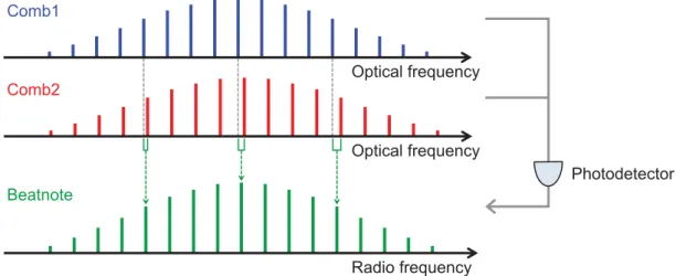
Fig. 1.5: Dual-comb in the terahertz scale and comb-like beatnote in the megahertz scale. Two combs with slightly diﬀerent repetition frequencies are down-converted to the beatnote signal by detecting with a photodetector. The beatnote is useful to monitor the absorption and other variations through the dual-comb light. This is because each comb line in the terahertz scale corresponds to the each beatnote line in the megahertz scale, that is compatible with electrical equipments.

1.4.3 Cross-phase modulation between dual-comb

Optical frequency comb sources (and also optical pulses sources) have pulse trains in the time domain and broadband spectrum in the frequency domain. The paired comb source having slightly diﬀerent repetition frequencies, that is known as dual-comb, can provide advantages such as high resolution, high sensitivity, and high data acquisition speed in optical spectroscopy and ranging. For example, the scan rate of a dual-comb spectrometer is several orders of magnitude faster than that of a Fourier transform spectrometer using a Michelson interferometer. This is because the second comb in a dual-comb system works as a reference and scan the delay automatically, instead of mechanically scanning the mirror in a Michelson interferometer. In the frequency domain, two combs in the terahertz scale can be down-converted to comb-like beatnote signal in the megahertz scale by detecting with a photodetector as shown in Fig. 1.5.

In a dual-comb system, which utilizes two types of optical pulse trains with slightly diﬀerent repetition frequencies, microcomb platforms can achieve fast scan rates for spectroscopy [55,57] and LiDAR [60, 61]. This is because a dual-comb system with optical pulse trains at high repetition frequencies can allow the large diﬀerence between the repetition frequencies, which corresponds to the scan rate in measurement systems, with low noise. Hence the key parameter is the repetition frequency of each soliton microcomb in the time domain, which corresponds to the mode spacing between comb lines in the frequency domain.

Recently, dual-comb generation in a single microresonator attracts much attention [55, 57, 61, 107–112] for dual-comb applications including spectroscopy and LiDAR. An experimental demonstration of dual-comb solitons in a single microresonator has been realized by utilizing clockwise and counter-clockwise directions [90] and spatially diﬀerent transverse modes [111]. However, it is still challenging to generate dual-comb solitons because the two propagating

(22)

solitons interact and result in modulation of repetition frequencies through cross-phase modu-lation (XPM). XPM is one of Kerr eﬀects and modulates the phase of one light with another light. In addition, although a theoretical model that takes account of XPM and the diﬀerence between repetition frequencies has been developed [108], the results of simulation and analysis for dual-comb solitons have not been well considered.

1.5 Motivation and chapter overview

A microcomb is formed inside a microresonator via FWM, which is driven by a CW pump laser. However, besides the FWM processes, other effects of optical nonlinearities occur owing to strong light-matter interactions in the dielectric microresonator. These effects sometimes help or disturb to generate a microcomb, and also change the properties including the repetition frequency, bandwidth, and coherence. In this thesis, the author studies the effects of cavity optomechanics, SRS, and XPM on microcombs. These understandings help to generate micro-combs that have controlled-properties such as noises, operation wavelengths, spectral envelope shapes, and repetition frequencies.

This thesis consists of seven chapters and is organized as follows:

Chapter 1 introduces the background to microresonators and microcombs to clarify the motivation behind this thesis. The basic generation scheme, previous researches, and microcomb applications are introduced. In addition, the related researches of eﬀects of optical nonlinearities on microcombs are introduced.

Chapter 2 explains microresonator characteristics to make it easier to understand this thesis. The contents are basic theory of microresonators, optical coupling systems, fabrication processes of microresonators and tapered ﬁbers, developed measurement methods for Q factors and cavity dispersions, and optical nonlinear processes in microresonators.

Chapter 3 explains the basic theory and measurement data of microcombs. The theory mainly deals with a Lugiato-Lefever equation (LLE), which can calculate microcomb formation inside a microresonator and provide an approximate analytical solution for a dissipative Kerr soliton. The measurement data includes microcomb spectra generated in three platforms (silica toroid, silica rod, and polished magnesium ﬂuoride microresonators) and optical transmission with soliton steps while scanning the pump frequency.

Chapter 4 describes a study of cavity optomechanical behaviors on microcomb generation and demonstrates that it is possible to suppress cavity optomechanical parametric oscillations with the generation of a Turing pattern comb (microcomb) in an anomalous dispersion toroidal microresonator.

Chapter 5 describes a study of Raman comb generation in a silica rod microresoator that has a cavity FSR in a microwave rate. The center wavelength is controlled via detuning and coupling optimizations. This study provides the explanation of the formation dynamics, of which understanding is needed to generate smooth and phase-locked Raman combs.

Chapter 6 is a numerical study of dual-comb generation and soliton trapping in a single microresonator, whose two transverse modes are excited with orthogonally polarized dual-pumping. The simulation model is described by using coupled LLEs, which take account of

(23)

1.5. Motivation and chapter overview XPM and the diﬀerence in repetition frequencies.

Chapter 7 summarizes the content of each chapter and discusses future work and the outlook for microcomb research.

(24)

(25)

Chapter 2 Optical microresonators

This chapter explains microresonator characteristics to make it easier to understand this thesis. The contents are basic theory of microresonators, optical coupling systems, fabrication processes of microresonators and tapered ﬁbers, developed measurement methods for Q factors and cavity dispersions, and optical nonlinear processes in microresonators.

2.1 Microresonator characteristics

2.1.1 Basic microresonator parameters

Resonance frequencies

Optical resonators have the discrete resonance frequency ω_m, which is related to the optical cavity length nL. m is the mode number (m ∈ N), n is the eﬀective refractive index, and L is the cavity length. The internal electric ﬁeldE(z,t)is written as

E(z,t)= E0exp{i(kz−ωmt)}, (2.1)

whereE0is the amplitude and k is the propagation constant. Since the phase of resonant light shifts 2πmper roundtrip (k L = 2πm), the resonance wavelengthλ_m and angular frequencyω_m satisfy the following equations:

λm = nL

m , (2.2)

ωm = 2πmc

nL . (2.3)

Here c is the speed of light. In the case of no dispersion (i. e. the eﬀective refractive index does not depend on the frequency), the resonance frequencies have an equal mode spacing D1 (in units of rad·Hz) as follows: ω_m = mD1. The cavity FSR is inverse to the roundtrip time as

t−1

r = D1/2πand the optical cavity length has the relation to the roundtrip time asctr = nL. The series of the resonance modes are known as transverse mode or mode family, and have the same mode proﬁle and the polarization.

(26)

Cavity dispersion

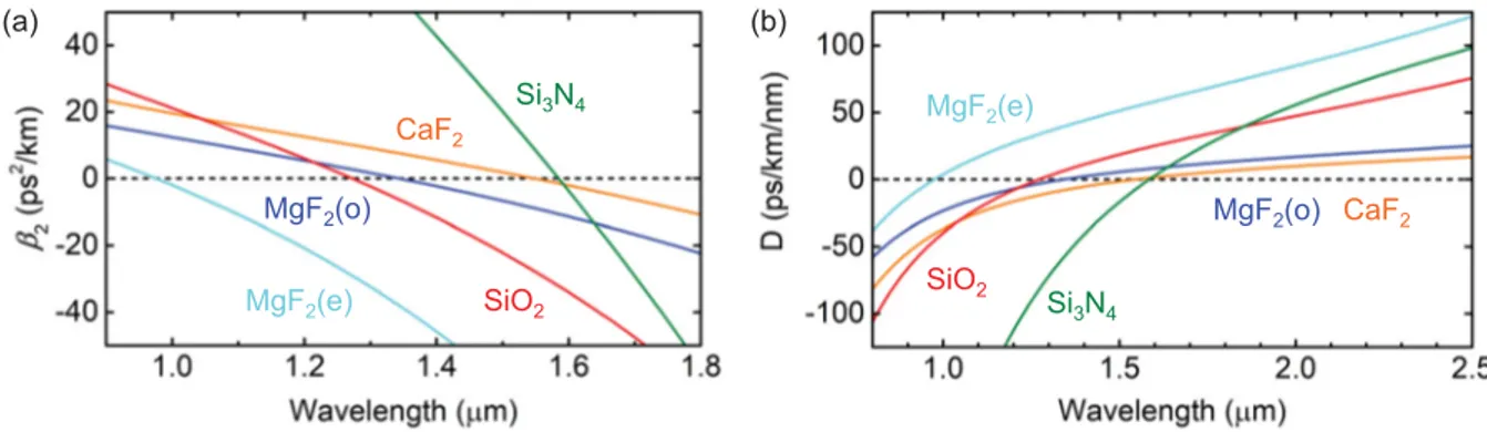
The cavity dispersion is a parameter to represent that the effective refractive index depends on the frequency, the resonance mode profile, and the polarization in a microresonator. Hence, cavity dispersion is determined by the material and geometrical dispersions. The material dispersion follows a Sellmeier equation that determines the refractive index in the medium. The geometrical dispersion can be controlled by changing the microresonator structure because the mode profiles have different occupancies of optical intensity inside the medium. For example, a large amount of evanescent fields outside the microresonator leads to less effective refractive index.

As explained above, resonance frequencies have equal mode spacings when not taking account of cavity dispersion. However, cavity dispersion changes the mode spacings depending on the frequency. The resonance frequencies can be expressed with a relative mode number μ (μ∈Z) that is obtained from the absolute mode numberm. The center mode number is deﬁned as μ = 0, which corresponds to the pump mode for microcomb generation. The resonance angular frequencyω_μ and the frequency fμare written with Taylor-expanded equations:

ωμ =ω0+D1μ+ 12D2μ 2₊ 1 6D3μ 3₊_{· · ·} =ω0+D1μ+Dint(μ), (2.4) fμ = f0+d1μ+ 1₂d2μ2+ 1₆d3μ3+· · · = f0+d1μ+dint(μ). (2.5)

Figure 2.1 is an illustration to explain Eq. (2.4). D1 is the cavity FSR that means light in the frequencyω0circulates in the microresonator at the roundtrip timetr = (D1/2π)−1. D2andD3 represent second and third order dispersion, respectively. Dintincludes all dispersion terms. The higher order dispersion can be neglected in many cases because of the relation: D2D3 · · ·. The important point for microcomb generation is the sign ofD2, whereD2> 0 (D2 < 0) denotes anomalous (normal) dispersion.

In many optical ﬁber researches, dispersion is expressed with group velocity dispersions (β2

1 2 + ⋯ 1 2 + ⋯ 1 2 + ⋯ 1 2 + ⋯ = −1 = −2 = 0 = 1 = 2 > 0: Anomalous dispersion < 0: Normal dispersion = + +1 2 + ⋯ Resonance

Fig. 2.1: Resonance frequencies taking cavity dispersion into account. This ﬁgure summarizes Eq. (2.4). Gray Lorentzian shapes represent resonance modes whose positions are diﬀerent from black dashed lines (that have equal spacings) due to the cavity dispersion.

(27)

2.1. Microresonator characteristics andβ3), which are related toD1andD2values:

β2= −nD2 cD2 1 , (2.6) β3= 3nD22 cD4 1 − nD3 cD3 1 ≈ − nD3 cD3 1 . (2.7)

Cavity dispersion is a critical parameter in microcomb research for the initial comb genera-tion, comb bandwidth, and mode-locking. The methods of measurement and calculation are introduced in §2.4.

Cavity decay rate and quality factor

The performance of each resonance mode is expressed with a cavity decay rate κ, which is related to an intrinsic decay rate κi and a coupling rate to the external waveguide κc as follows: κ = κi+ κc. The intrinsic decay rate includes loss factors including scattering at the microresonator surface, absorption and scattering inside the material, and the radiation at the bending points. The coupling eﬃciency is determined by the relation between the intrinsic decay rate and the coupling rate (the detail is explained in §2.1.2). The intracavity optical energy

Ucav(t)decays exponentially:

Ucav(t)=Ucav(0)exp(−κt). (2.8)

In general, the performance of a resonator is expressed with a quality factor (Q factor)Qand a ﬁnesseF. A Q factor is deﬁned as

Q=2π (Intracavity optical energy)

(Energy loss per optical cycle) =2π

Ucav(t)

−Ucav(t) dt 2ωπ0

= ω0_κ . (2.9)

Hence a Q factor can be determined by the cavity decay rate κ in the time domain, which corresponds to the full width at half maximum (linewidth) of the resonance mode in the frequency domain. The shape of a resonance mode is a Lorentzian function, which is explained in §2.1.2. The photon lifetimeτcavis defined asτcav = κ−1, which can be evaluated by the decay of output power from a microersonator in the time domain. The finesse is defined asF = D1/κ, where

F 1 denotes that each resonance mode can be distinguished.

Eﬀective mode area

One advantage of microresonator platforms is to confine light in the small area and volume. The effective mode areaAeff is determined by a resonant mode profile:

Aeﬀ =

(∬ |E|2dA)2

∬

|E|4_dA , (2.10)

where|E|2_{corresponds to the optical intensity. The eﬀective mode volume}_V

effcan be expressed asVeff = AeffL.

(28)

2.1.2 Optical coupling to microresonators

࢙

_ܑܖ

ሺ࢚ሻ

࢙

_ܗܝܜ

ሺ࢚ሻ

ࢇ

_૙

ሺ࢚ሻ

Microresonator Waveguide

ࣄ

_܋

ࣄ

_ܑ

Fig. 2.2: Optical coupling system between a microresonator and a coupling waveguide. a0(t)is the intracavity ﬁeld, sin(t)andsout(t)are the input and output ﬁelds, respectively. κi andκcare the intrinsic decay and coupling rates, respectively.

Optical input and output between a microresonator and a coupling waveguide are performed through an evanescent field. The typical coupling waveguides are optical tapered fibers, pigtailed fibers, prisms, and on-chip waveguides. A coupled mode equation for single resonance mode is written with a light field A0(t), which is normalized as that|A0(t)|2corresponds to the number of intracavity photons at the resonance frequencyω0as

dA0(t) dt =− κ 2A0(t) −iω0A0(t)+ √_κc sin(t)exp(−iωpt), (2.11) wheresin(t)is the input ﬁeld to the waveguide andωpis the pump frequency. Then, the phase transformation is applied asa0(t)= A0(t)exp(iωpt)that can rewrite Eq. (2.11) to

da0(t) dt =− κ 2a0(t)+i(ωp−ω0)a0(t)+ √ κcsin(t). (2.12)

In addition, the output ﬁeldsout(t)is given by

sout(t)=√κca0(t) −sin(t). (2.13)

For the stationary-state analysis, the left-hand side in Eq. (2.12) is set to zero anda0(t), sin(t), andsout(t)in Eqs. (2.12) and (2.13) are regarded as time independent. Equations (2.12) can be transformed to a0 = √_κc 1 2κ−iΔω0 sin, (2.14) |a0|2 = ₁ κc 4κ2+Δω 2 0 |sin|2, (2.15)

where Δω0 = ωp− ω0. Equations (2.14) and (2.15) represent the relation between the in-tracavity and input ﬁelds. Since |a0|2 corresponds to the number of photon stored inside the

(29)

2.1. Microresonator characteristics

(a) (b)

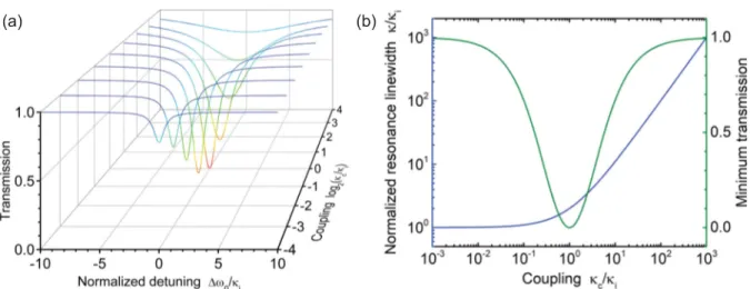
Fig. 2.3: Calculation results with Eq. (2.15). (a) Transmission of resonance modes as a function of a coupling parameter. κc/κi = 1 represents a critical coupling condition. (b) Normalized resonance linewidth (blue) and minimum transmission (green) as a function of a coupling parameter.

microresonator, the intracavity optical power Pcav can be obtained from Eq. (2.15). Also, the optical power in the coupling waveguide (Pin and Pout) can be obtained from |sin|2 and |sout|2 that correspond to the number of photons passing the waveguide per second.

Pcav = ωp|a0|2× (D1/2π), (2.16)

Pin(out) = ωp|sin(out)|2, (2.17)

where is the Planck constant devided by 2π. In experiments, microresonators are evaluated by monitoring the relation between input and output ﬁelds, which provides parameters of the cavity linewidth, transmission, and phase response:

sout sin = 1 2(κc−κi)+iΔω0 1 2(κc+κi) −iΔω0 = 1 2( κc κi −1)+i Δω0 κi 1 2( κc κi +1) −i Δω0 κi , (2.18) sout sin 2= 1 4(κc−κi)2+Δω20 1 4(κc+κi)2+Δω 2 0 = 1 4( κc κi −1) 2₊₍Δω0 κi ) 2 1 4( κc κi +1) 2+(Δω0 κi ) 2 . (2.19)

In this thesis, I use the coupling parametersηandKthat are deﬁned asη= κc/κandK = κc/κi,

respectively. The optical coupling is distinguished in three conditions: under (K < 1,η < 0.5), critical (K = 1, η = 0.5), and over (K > 1, η > 0.5) coupling conditions. The transmission of a resonance is described by Eq. (2.18), whose calculation examples are shown in Fig. 2.3. As shown in Eq. (2.18) and Fig. 2.3, the transmission has a Lorentzian function, which can be transformed from an exponential function by using Fourier transformation. By considering the build-up eﬃciency, critical coupling is an ideal condition, which can be optimized by controlling the coupling rateκc. Figure 2.4 shows transmission (blue) and phase (red) of a resonance mode in three coupling conditions (under, critical, and over coupling).

(30)

κc/κi= 0.5 (under coupling) κc/κi= 1 (critical coupling) κc/κi= 2 (over coupling)

Fig. 2.4: Calculation results with Eqs. (2.14) and (2.15) in three diﬀerent coupling conditions. The blue and red lines represent the transmission and the phase, respectively.

2.2 Fabrication of microresonators used in this thesis

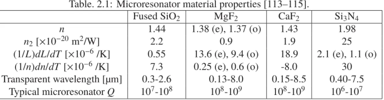
In this thesis, I use three types of microersonators to generate microcombs: silica toroid, silica rod, and polished MgF2microresonators. This section explains the fabrication processes. Table 2.1 introduces the material properties of silica, MgF2, and other commonly used optical materials.

2.2.1 Silica toroid microresonators

Silica toroid microresonators were developed in 2003 by California Institute of Technology (Caltech) [17] and used to demonstrate equally spaced microcomb generation in the ﬁrst impor-tant report in 2007 by Max-Planck-Institute for Quantum Optics (MPQ) [5]. The advantages of a toroid microresonator are on-chip fabrication, a high-Q (~100 million), and a small mode volume. Carbon dioxide (CO2) laser reﬂow processes make the smooth toroidal surface that reduces scattering losses and achieves a high-Q.

Figure 2.5 shows the fabrication processes of a toroid microresonator, including photolithog-raphy, silicon etching with xenon difluoride (XeF2), and CO2 laser reflow. First, (a) a silicon wafer with an silica layer of 2 μm thickness is prepared. Second, (b) photolithography and silica etching with a buffered hydrogen fluoride (HF) forms circular silica disks on the silicon wafer. The reaction is expressed as SiO2+ 6HFH2SiF6+ 2H2O. The silica disk have diameters that are typically from 50 to 200 μm. Third, (c) silicon etching with XeF2forms the structure of a

Table. 2.1: Microresonator material properties [113–115].

Fused SiO2 MgF2 CaF2 Si3N4

n 1.44 1.38 (e), 1.37 (o) 1.43 1.98

n2[×10−20m2/W] 2.2 0.9 1.9 25

(1/L)dL/dT [×10−6/K] 0.55 13.6 (e), 9.4 (o) 18.9 2.1 (e), 1.1 (o) (1/n)dn/dT [×10−6/K] 7.3 0.25 (e), 0.6 (o) -8.0 30 Transparent wavelength [μm] 0.3-2.6 0.13-8.0 0.15-8.5 0.40-7.5

(31)

2.2. Fabrication of microresonators used in this thesis silica disk on a silicon pillar, which can conﬁne light in a whispering-gallery mode at the edge of the silica disk. This reaction follows 2XeF2+ Si2Xe+SiF4. Optimizing the ratio between diameters of the silica disk and the silicon pillar is a key to achieve a high-Q after forming the toroidal shape. Finally, (d) the CO2 laser beam that is exposed to the silica disk from the top can melt only the edge of the silica disk because the silicon pillar works as a heat sink. The laser reﬂow process forms the toroidal shape that has a smooth surface. Typically, the Q factor improves from hundreds thousand in a disk to tens million in a toroid.

Si SiO2

(a) (b) (c) (d)

Photolithography Silicon etching Laser reflow

SEM images Optical microscope images

50 μm 50 μm

Fig. 2.5: Fabrication processes of a silica toroid microresonator. Optical microscope and scanning electron microscope (SEM) images are shown for each fabrication step. (a) Silicon wafer with a silica layer of 2 μm thickness. (b) Circular silica disk on the silicon wafer. (c) Circular silica disk on a silicon pillar. (d) Silica toroid microresonator, whose toroidal shape is formed at the edge of the silica disk by using a CO2laser reﬂow process.

50 μm 50 μm

(32)

2.2.2 Silica rod microresonators

Silica rod microresonators were developed in 2013 by National Institute of Standards and Technology (NIST) [116], which have the advantage of high-Q achievability (over 100 million), easy fabrication processes, and a wide range of cavity FSR that covers from a few to hundreds of gigahertz.

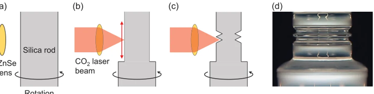
Figure 2.7 shows the fabrication processes of a silica rod microresonator. First, (a) a silica rod containing low OH (<10 ppm) and other impurities is prepared and mounted on an air spindle. Second, (b) a CO2laser beam is focused on the silica rod surface with a zinc-selenide lens (50 mm focal length) while the silica rod rotates. By scanning the focusing position along to the rod axis, a diameter of the microresonator can be controlled by melting the material. Finally, (c) the CO2laser beam is focused on the two positions of the silica rod and forms the resonator shape as shown in Fig. 2.7(d). In the steps of (b) and (c), becoming clouded in silica should be avoided because it reduces the Q. The clouded silica can be observed at other than the resonator part in Fig. 2.7. (a) (b) (c) ZnSe lens Rotation Silica rod CO2laser beam (d)

Fig. 2.7: Fabrication processes of a silica rod microresonator. (a) Silica rod is mounted and rotated on an air spindle. (b) CO2laser beam is focused on the surface of the silica rod. The focus position is scanned to melt the silica and control the diameter. (c) Microresonator structure is formed by focusing the laser beam at two positions. (d) Optical microscope image of a silica rod microresonator.

2.2.3 Polished magnesium ﬂuoride microresonators

Polished magnesium fluoride (MgF2) microresonators are ultrahigh-Q microresonators, which were used to demonstrate soliton microcomb generation in the first important report by EPFL [39]. This microresonator has the advantages of ultrahigh-Q (~1 billion) and high thermal stability thanks to its small thermo-optic coefficient. On the other hand, it is difficult to fabricate microresonators with a small diameter because of hand-cutting and polishing processes.

Figure 2.8 shows the fabricated MgF2microresonators that have diameters of 3.95 mm (left) and 4.17 mm (right)1. The fabrication processes follow three steps. First, a cylindrical base material of a few mm diameter is cut out from a bulk material (e.g. commercial MgF2lenses).

1The MgF2 microresonators used in this thesis were fabricated by M. Fuchida and A. Kubota. The images in

(33)

2.3. Tapered ﬁber coupling and quality factor measurement The base material is glued to a metal post and mounted on an air spindle. Second, the rotated base material is roughly shaped to the microresonator structure by grinding with a diamond turning. Third, the smooth microresonator surface is created by polishing with diamond particles while decreasing the particle sizes (3, 1, 0.25, and 0.05 μm), which can lead to a ultrahigh-Q.

1 mm 1 mm

Fig. 2.8: Optical microscope images of polished MgF2microresonators.

2.3 Tapered ﬁber coupling and quality factor measurement

Whispering-gallery modes can be excited through an evanescent field by using an external waveguide such as an optical tapered fiber, a pigtailed fiber, and a prism. In this thesis, a tapered fiber was used to couple light into silica toroid, silica rod, and MgF2microresonators. The tapered fiber coupling has the advantages of high coupling efficiency (over 99 %), almost lossless propagation in the tapered fiber, and a lot of flexibility of the coupling position controlled by using a three-axis stage.

2.3.1 Fabrication of tapered ﬁbers

A tapered fiber is fabricated by heating and stretching a commercial single-mode optical fiber. The smallest part of the tapered fiber has a diameter of around 1 μm (a single-mode fiber has the clad diameter of 125 μm), which is the same order as the laser wavelength (~1.55 μm) to present an evanescent field outside the fiber.

Figure 2.9(a) shows the fabrication setup where a single-mode fiber is heated with a gas torch on two one-axis automatic positioning stages. The gas torch employs oxygen (O2) and propane (C3H8) gases to burn. The heating position on the fiber is repeatedly scanned while pulling the fiber at the speed of 140 μm/s.

Figure 2.9(b) shows the transmission of an input laser while pulling the optical fiber. Typi-cally, more than 95% of transmission in the fabricated tapered fiber can be achieved by optimizing the positions of the fiber, torch, and two stages that hold the fiber. The oscillation amplitude de-pends on the propagation mode at the thinnest point of the fiber, as described in Fig. 2.9. Hence, pulling the fiber can be stopped when the fiber diameter becomes around 1 μm by monitoring the oscillation amplitude. While pulling the fiber, there are three propagation modes. First, the propagation mode is supported by the total internal reflection between the core and clad of an optical fiber, which is the general scheme to confine light in a commercial single-mode fiber.

(34)

Second, heating and stretching crush the core that changes to the mode confined between the clad and air. In this condition, the propagation mode profiles (in a multi-mode) continuously change during pulling the fiber, that causes the transmission oscillation. Finally, since the number of propagation modes becomes one (in a single-mode), the transmission oscillation is suppressed. The diameter can be calculated with the V number (Vnum) because the propagation mode is supported in a step-index fiber structure (between the core and air). The V number is expressed as Vnum = πφfibern2 1−n 2 2 λ , (2.20)

whereφfiberis the diameter of the tapered fiber,λis the laser wavelength, andn1andn2are the refractive indices inside and outside the waveguide, respectively. In a step-index fiber, the single-mode condition is obtained when the V number is 2.405. Therefore, the transmission oscillation is suppressed when the diameter of tapered fiber becomes smaller thanφfiber= 1.15 μm, which is calculated withn1= 1.44,n2 =1, andλ= 1.55 μm.

Single mode (core-clad) Multi mode (clad-air) Single mode (clad-air) (b) (a)

Fig. 2.9: (a) Tapered fiber pulling setup. (b) Transmission during heating and pulling the optical fiber. The amplitude oscillation indicates change of the propagation mode, which includes a single- and a multi-mode. When decreasing the oscillation, the pulled optical fiber has a diameter of around 1 μm, which is compatible with coupling light to a microresonator.

2.3.2 Quality factor measurement with a tapered ﬁber

The Q factor is an important parameter to evaluate whether the microresonator could build up intracavity optical power and cause optical nonlinear effects. The Q factor is determined by using the cavity decay rate following Eq. (2.9), which can be evaluated by measuring the linewidth of a resonance mode in the frequency (wavelength) domain and the photon lifetime in the time domain. Figure 2.10(a) shows the tapered fiber coupling setup to measure Q factors. A toroid chip is placed on a three-axis automatic positioning stage that can control the relative position between the microresonator and fiber. The coupling position is monitored by using microscopes from the top and side, whose views are shown in Figs. 2.10(b) and (c). Figure 2.11

(35)

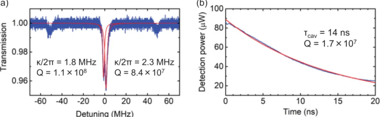
2.3. Tapered ﬁber coupling and quality factor measurement shows experimental setups used for Q factor measurement in (a-c) the frequency and (d,e) the time domains. Figures 2.12, 2.13, and 2.14 show measurement results with a silica toroid, a silica rod, and a MgF2microresonators, respectively. Fabricated microresonators in this thesis have Q factors of typically 1-10 million (silica toroid), 10-100 million (silica rod), and 100-1000 million (MgF2).

Frequency domain measurement

As explained in §2.1.2, the transmission in a resonance mode has a Lorentzian shape as a function of the detuning between the resonance and laser frequencies. Therefore, the linewidth of a resonance mode can be evaluated by monitoring the transmission while scanning the laser frequency. Here the frequency (wavelength) axis needs to be calibrated with some frequency (wavelength) marker, that are created by using the built-in function of a commercial laser (Santec TSL-510 and TSL-710), a ﬁber Mach-Zehnder interferometer (MZI), and a phase modulator. For example, Figs. 2.12(a) and 2.13(a) show measured resonance modes with 50 MHz modulated sidebands that can calibrate from a time axis in an oscilloscope to a frequency axis. As written in §2.1.1, a Q factor is determined asQ = ω0/κ(= λ0/Δλ), where λ0is the resonance wavelength andΔλis the linewidth in the wavelength domain. The frequency calibration in a broad wavelength range, which is created with a ﬁber MZI, can also be used to measure cavity dispersions. The detail is provided in §2.4.2.

Time domain measurement

Q factors can be evaluated in the time domain by monitoring the output power after stopping the laser input to the resonance mode. The output power decreases exponentially and its decay rate corresponds to the cavity decay rate. This scheme is compatible with ultrahigh-Q microresonators (Q ≥ 108) because of their long photon lifetime (corresponding to the small cavity decay rate). In this thesis, I used two methods in the time domain measurement, which are shown in Figs. 2.11 (d) and (e). In Fig. 2.11 (d), the laser frequency is scanned over the resonance mode. The scan speed (vscanin units of rad·Hz/s) needs to satisfy withτcav κ/vscan. After going across the resonance, the output of conﬁned light from the microresonator interferes with the input laser that generate an interferometer signal. In Fig. 2.11 (e), the coupled laser power is modulated with an intensity modulator, where a squared signal is applied. The cavity decay rate can be obtained by ﬁtting with an exponential function to the signal amplitude.

(36)

(a) (b) (c) Top camera Side camera ~ 1 μm Toroid chip Tapered fiber

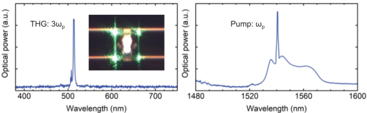
Fig. 2.10: (a) Tapered ﬁber coupling setup. The toroid chip is placed on a three-axis automatic positioning stage. The toroid microresonator is placed at the blue-emitted point on the chip in the picture (through THG). (b)(c) The microscope views from the top and the side.

FPC TLD PWM DAQ TLD OSC MZI FPC PD FG FG FG TLD FPC PM OSC PD TLD FPC FG OSC PD (a) (b) (c) (d) (e) TLD FPC IM PD OSC FG

Fig. 2.11: Experimental setups for Q factor measurement in (a-c) the frequency and (d,e) the time domains. TLD: tunable laser diode, FPC: ﬁber polarization controller, PWM: power meter, DAQ: data acquisition, FG: electrical function generator, MZI: ﬁber Mach-Zehnder interferometer, PD: photodetector, OSC: oscilloscope, SG: electrical signal generator, PM: phase modulator, IM: intensity modulator, PPG: pulse pattern generator.

(37)

2.3. Tapered ﬁber coupling and quality factor measurement κ/2π = 2.3 MHz Q = 8.4㽢107 (a) (b) τcav= 14 ns Q = 1.7㽢107 κ/2π = 1.8 MHz Q = 1.1㽢108

Fig. 2.12: Q factor measurement of silica toroid microresonators in (a) the frequency and (b) the time domains. (a) The phase modulated laser with 50 MHz bandwidth is scanned over the resonance mode (blue). Around the center dip, the two small dips can be observed that can be used to calibrate the frequency axis. Red lines represent Lorentzian functions, whose linewidths correspond to the cavity decay rates κ/2π (here: 1.8 and 2.3 MHz). The splitting is cause by the mode coupling between clockwise and counter-clockwise propagation modes. (b) Optical output power, which decreases exponentially, is monitored after turning the laser input oﬀ.

(a) (b)

τcav= 0.52 μs Q = 6.3㽢108

κ/2π = 860 kHz Q = 2.2㽢108

Fig. 2.13: Q factor measurement of silica rod microresonators in (a) the frequency and (b) the time domains. (a) The phase modulated laser with 50 MHz bandwidth is scanned over the resonance mode. (b) The input laser is scanned over the resonance at the scan speed (vscan in units of rad·Hz/s) that satisﬁes with τcav κ/vscan. The interference signal can be observed while light is output from a microresonator.

τcav= 1.24 μs Q = 1.5㽢109

(38)

2.3.3 Control of coupling condition between microresonator and ﬁber

To control the coupling condition between resonance and fiber modes is an important technique to input the laser light efficiently. The basic theory is explained in §2.1.2. In experiments, the coupling condition can be optimized by selecting the optimum diameter of a tapered fiber and controlling the relative position between the microresonator and tapered fiber [117–119]. Figure 2.15 shows measurement results of normalized resonance linewidths and minimum transmissions as a function of (a) the gap distance between the fiber and the toroid microresonator, and (b) the coupling parameter. Since the diameter of the tapered fiber at the coupling point is properly selected, the transmission reaches close to zero at the gap distance of 0.9 μm. A critical coupling condition, where the transmission is zero and κ/κi= 2, is suitable for most of microresonator experiments because input laser light is efficiently coupled to a resonance mode. When the diameter is not properly selected, the transmission cannot reach zero due to the phase mismatch between resonance and fiber modes.

(a) (b)

Experiment Theory

Fig. 2.15: Measurement of normalized resonance linewidths and minimum transmissions as a function of (a) the gap distance between the ﬁber and toroid microresonator and (b) coupling parameter. (a) The critical coupling, where the transmission is zero andκ/κi= 2, is obtained at the gap distance of 0.9 μm. (b) Experimental data is in good agreement with the theory, which is calculated by using Eq. (2.15).

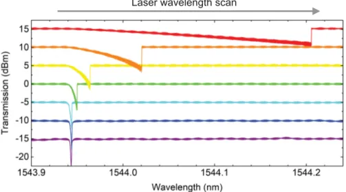
2.3.4 Thermally induced resonance shift

Thermal effects inside a microresonator have impacts on optical coupling, Q factor measurement, output noises, and other properties. For example, in order to evaluate Q factors exactly, resonance frequency shift by thermo-optic and thermal expansion effects should be avoided by reducing the input laser power. This is because the measured resonance shape is distorted from a Lorentzian shape. Figure 2.16 shows resonance modes, which are measured by scanning the pump wavelength from short to long, in a silica toroid microresonator with various input laser powers. With a higher input power, the shape of the resonance mode changes from Lorentzian to triangular. This frequency shift depends on changes of the effective refractive index and the