RELATIVE RISK OF DISEASE USING
GENERALIZED LINEAR MIXED MODEL
1Kismiantini
Department of Mathematics Education,Yogyakarta State University Karangmalang, Yogyakarta 55281, Indonesia
e-mail: [email protected]
Abstract
A traditional approach to measure a relative risk of disease is standardized mortality ratio (SMR). SMR is the ratio of observed number of count in an area and expected number of count in an area. The number of count in an area are assumed to have independent Poisson distribution. SMR has the greatest uncertainty (when disease is rare and/or small geographical area), because they have small population and large of standard error. Statistical smoothing might solve that problem by borrowing strengthness (precision) of other data, such as a bayesian approach with poisson-gamma model. If random area effect is included into the Poisson-gamma model, estimation to risk relative will be obtained difficulty. Generalized linear mixed model is an alternative approach to solve the problems to get a relative risk of disease.
Keywords: relative risk, generalized linear mixed model
1. Introduction
A method for displaying the geographical distribution of disease occurrence is disease mapping. The aim of disease mapping is obtain relative risk estimates for each study area (Wakefield, 2006). The traditional approach to measure a relative risk of disease is standardized mortality ratio (SMR). However, this approach has been criticized. One of criticism is the instability of the crude SMR, especially when rare diseases are investigated in an area with small population. In such a case, both the observed and the expected values are low. As a result, an area with a small population tends to present an extreme SMR, yielding a map which is dominated by the least reliable information (Bernardinelli & Montomoli, 1992).
Many researchers have sought an alternative solution for SMR problems. Empirical Bayes (EB) estimation (using Poisson-gamma model, the log-normal model and the CAR-normal model) provides a more stable risk estimate such as leading to a smooth map with fewer extremes in the relative risk estimate (Clayton & Kaldor, 1987). Wakefield (2006) proposed a simple Poisson-gamma two stage model that offers analytic tractability and ease of estimation and is useful for exploratory analyses using empirical Bayes method. If area random effect is included into the Poisson-gamma model,
1
estimation to relative risk will not tractable. Generalized linear mixed model is an alternative approach to solve that problem. The methods are illustrated using diabetes data to get relative risk of disease.
2. Standardized Mortality Ratio (SMR)
The most common of summary measure of health outcomes for disease mapping is standardized mortality ratio (SMR). If Yi is the number of incident cases in county i
and Ei is the expected number of incident cases, =
=
risk to each county and is a random variable,
(
i i)
Then the ratio of observed to expected counts (Yi Ei ) is the standardized mortality ratio.
The ratio
θ
ˆi =Yi Ei is obtained by maximizing likelihood function. This SMR is an unbiased maximum likelihood estimator. The variance of the estimatoris
( )
3. Generalized Linear Mixed Model
Generalized Linear Mixed Models (GLMM), assume normal (Gaussian) random effects. Conditional on these random effects, data can have any distribution in the exponential family (McCullogh & Searle, 2001). The exponential family comprises many of the elementary discrete and continuous distributions. The binary, binomial, Poisson, and negative binomial distribution, for example, are discrete members of this family. The normal, beta, gamma, and chi-square distributions are representatives of the continuous distributions in this family.
The basic model of GLMM is suppose that Yrepresents the
(
n×1)
vector ofThe GLMM contains a linear mixed model inside the inverse link function. This model component is referred to as the linear predictor,
Z
X +
=
The variance of the observations, conditional on the random effects is
variance function a
( )
µ =µ2 and[ ]
=µ
2φ
Y
Var . If =0andR =φI, the GLMM
reduces to a generalized linear model (GLM) or a GLM with overdispersion.
4. Relative Risk of Disease Using Generalized Linear Mixed Model
Let Yi is the response of the ith county and let assumed that Yi has probability
function belonging to the Poisson distribution withEiθi. Then the model for the region-specific relative risk using GLMM is (Breslow & Clayton, 1993)
{
i}
i mi =exp ′ +γ , =1, ,
θ X
Since the mean of the Poisson variates, conditional on the random effectsµi =Eiθi, applying a log link yields
{ }
µi =log{ }
Ei +X′ +γi logwhere the term log
{ }
Ei is an offset, is a vector of coefficients regression, X is a matrixof independent variables as fixed effects, and the γi are area random effects,
(
2)
, 0
~ σ
γi N .
5. Data Analysis
Diabetes disease data is used to illustrate the generalized linear mixed model to estimate the relative risk of disease. The data is obtained from “Puskesmas Srandakan” for 2007 year. The data is taken from 50 villages at Bantul municipality. A variable of interest is a relative risk of diabetes disease, response variable Yi is number of risk of diabetes in the i-th villages, ni is number of people in the i-th villages, and Ei is expected number of risk of diabetes in the i-th villages. The standardized mortality ratio of θi is
given by
θ
ˆi =Yi Ei,where =i i i
i i
i n Y n
E . As covariates are average of age in the
i-th villages and average of sugar rate in the i-th.
Analysis of the data using SAS 9.1, PROC GLIMMIX to get ˆ , covariance parameter estimate, relative risks of disease and standard error for GLMM, and Ms EXCEL to get relative risks and standard error for SMR.
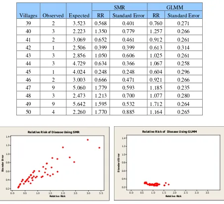
From Table 1 shows that a small population (small number of people in the ith village) has low expected counts, SMR and standard error are high (see 9th observation). Area with high population (high number of people in the ith village) has high expected counts, SMR and standard error are low (see 29th observation). Generally, SMRs have the greatest uncertainty because they have small population then standard error are high. Relative risks using GLMM provide a more stable risk estimate such as yielding low standard error than using SMR.
Table 1. Relative risk (RR) of diabetes disease based on SMR and GLMM
Villages Observed Expected
SMR GLMM
RR Standard Error RR Standard Error
Villages Observed Expected
SMR GLMM
RR Standard Error RR Standard Error
2 2 2.724 0.734 0.519 1.000 0.261
3 6 5.046 1.189 0.485 1.037 0.240
4 3 2.213 1.356 0.783 0.952 0.270
5 5 1.683 2.970 1.328 1.194 0.288
6 3 3.901 0.769 0.444 1.046 0.250
7 7 5.032 1.391 0.526 1.049 0.245
8 3 1.906 1.574 0.909 1.578 0.301
9 3 1.504 1.995 1.152 1.281 0.271
10 1 3.996 0.250 0.250 0.638 0.313
11 4 4.369 0.915 0.458 0.824 0.264
12 1 3.230 0.310 0.310 0.862 0.258
13 2 3.532 0.566 0.400 0.833 0.286
14 9 6.062 1.485 0.495 1.128 0.238
15 5 3.892 1.285 0.575 1.079 0.247
16 9 3.689 2.440 0.813 1.509 0.243
17 2 2.459 0.813 0.575 1.004 0.264
18 2 2.336 0.856 0.605 1.090 0.282
19 5 3.244 1.541 0.689 1.185 0.257
20 3 3.589 0.836 0.483 1.046 0.256
21 3 3.840 0.781 0.451 0.944 0.252
22 1 2.464 0.406 0.406 0.649 0.303
23 6 2.658 2.258 0.922 1.140 0.296
24 4 3.050 1.311 0.656 0.958 0.273
25 2 4.488 0.446 0.315 1.019 0.260
26 2 2.327 0.860 0.608 0.684 0.315
27 2 3.826 0.523 0.370 0.898 0.265
28 1 2.733 0.366 0.366 0.685 0.289
29 5 6.961 0.718 0.321 1.045 0.237
30 6 5.259 1.141 0.466 1.178 0.268
31 2 3.301 0.606 0.428 0.672 0.294
32 4 5.046 0.793 0.396 0.893 0.257
33 1 4.474 0.224 0.224 0.832 0.253
34 4 4.176 0.958 0.479 1.060 0.264
35 1 3.499 0.286 0.286 0.748 0.272
36 2 3.968 0.504 0.356 0.874 0.262
37 2 2.766 0.723 0.511 0.652 0.310
Villages Observed Expected
SMR GLMM
RR Standard Error RR Standard Error
39 2 3.523 0.568 0.401 0.760 0.271
40 3 2.223 1.350 0.779 1.257 0.266
41 2 3.069 0.652 0.461 0.912 0.261
42 1 2.506 0.399 0.399 0.613 0.314
43 3 2.856 1.050 0.606 1.025 0.261
44 3 4.729 0.634 0.366 1.067 0.258
45 1 4.024 0.248 0.248 0.604 0.296
46 2 3.003 0.666 0.471 0.921 0.266
47 9 5.060 1.779 0.593 1.185 0.235
48 3 2.473 1.213 0.700 1.077 0.280
49 9 5.642 1.595 0.532 1.712 0.264
50 4 2.260 1.770 0.885 1.164 0.265
Figure 1 shows that the relative risk increases as standard error increases. Figure 2 shows that the relative risk of disease using GLMM produced higher precision of estimate than SMR, because they have smaller standard error.
Table 2. Covariance Parameter Estimates
Covariance Parameter
Estimate Standard Error
Villages 0.07398 0.07016
Table 2 shows the estimate of the variance of the villages log-relative risks. There is significant village-to-village heterogeneity in risks. If the covariate were removed from the analysis, the heterogeneity in village-specific risks would increase. (The fitted SMRs in Table 1 were obtained without covariate X in the model).
6. Conclusions
The crude of SMR can reduce by inclusion covariates in the model. If there is significant county-to-county heterogeneity in relative risk, a Poisson regression analysis using GLMM can accommodate it.
7. References
Bernardinelli L. & Montomoli C. 1992. Empirical Bayes versus fully Bayesian analysis of geographical variation in disease risk. Statistics in Medicine 11: 983-1007.
Clayton D. & Kaldor J. 1987. Empirical Bayes estimates of age-standardized relative risks for use in disease mapping. Biometrics 43:671-681.
Kleinman, K., Lazarus, R. & Platt, R. 2004. A generalized linear mixed models approach for detecting incident clusters of disease in small areas, with an application to biological terrorism. American Journal of Epidemiology 159: 217-224.
McCulloch, C.E. & Searle S.R. 2001. Generalized, Linear, and Mixed Models. New York: John Wiley & Sons.
SAS Institute Inc. 2005. The Glimmix Procedure, Nov 2005. North Carolina: SAS Institute Inc.