AN UPPER BOUND ON THE REACHABILITY INDEX FOR A
SPECIAL CLASS OF POSITIVE 2-D SYSTEMS∗
ESTEBAN BAILO†, JOSEP GELONCH†, AND SERGIO ROMERO-VIV ´O‡
Abstract. The smallest number of steps needed to reach all nonnegative local states of a positive two-dimensional (2-D) system is the local reachability index of the system. The study of such a number is still an open problem which seems to be a hard task. In this paper, an expression depending on the dimensionnas well as an upper bound on the local reachability index of a special
class of systems are derived. Moreover, this reachability index is greater than any other bound proposed in previous literature.
Key words. Hurwitz products, Influence digraph, Local reachability index, Nonnegative ma-trices, Positive two-dimensional (2-D) systems, Reachability.
AMS subject classifications.93C55, 15A48, 93B03.
1. Introduction. Positive two-dimensional systems have received considerable attention in the last decade, as they naturally arise in different physical problems such as the pollutant diffusion in a river (see [16]), gas absorption and water stream heating (see [25]), among others. The structural properties of these 2-D state-space models have been recently analyzed in [18], [21] and [22].
One of the most frequent representations of positive 2-D systems is the Fornasini-Marchesini state-space model (see [17] and [18]) which is as follows:
xi+1,j+1=A1xi+1,j+A2xi,j+1+B1ui+1,j+B2ui,j+1
(1.1)
with local states x·,· ∈ Rn+, inputs u·,·∈ Rm+, state matrices A1, A2 ∈ Rn+×n, input
matrices B1, B2 ∈ Rn+×m and initial global state χ0 := {xh,k : (h, k)∈ C0} being
the separation setC0:={(h, k) : h, k∈Z, h+k= 0}. Let us denote this system by
(A1, A2, B1, B2).
If any nonnegative local state is achieved from the zero initial global state choosing a nonnegative input sequence, then the system is said to be locally reachable. Local
∗ Received by the editors September 19, 2007. Accepted for publication December 29, 2008. Handling Editor: Daniel Szyld.
†Departament de Matem`atica, Universitat de Lleida, Av. Alcalde Rovira Roure 191, 25198 Lleida, Spain ([email protected], [email protected]).
‡Institut de Matem`atica Multidisciplinar. Departament de Matem`atica Aplicada, Universitat Polit`ecnica de Val`encia, Val`encia, Spain ([email protected]). Supported by Spanish DGI grant number MTM2007-64477 and DPI2007-66728-C02-01.
reachability is equivalent to the possibility, in a finite number of steps, of attaining
each vector of the standard basis of Rn or alternatively a positive multiple of the
aforementioned vectors (see [18]).
The smallest number of steps needed to reach all local states of the system is the local reachability index of that system. This index plays an important role because it enables us to determine in a finite number of steps whether a system is locally reachable or not. Moreover, once this index is obtained, several new open problems could be addressed such as the study of reachability algorithms (see [4], [11] and [24]), of a canonical form by means of an appropriated positive similarity ([5] and [7]), of the definition of the pertaining complete sequence of invariants (see [5], [8] and [10]) as well as the analysis of this property under feedback ([6] and [20]) and so on.
The reachability index for positive 1-D systems has been studied in [5], [9], [14],
[15] and [26] among others, and it is always bounded byn(see [12] and [13]). However,
despite the numerous research efforts, an upper bound on such a number for a positive 2-D system is still an unanswered question.
With regard to this subject, different studies such as [18] and [23] have provided the first results, which have been revised in [2] and [3]. Lately, in [1], the local reachability index has been characterized for a particular class of positive 2-D systems, which are a generalization of the systems presented in [2] and [3], and an upper bound
on this index has been derived which even turns to be (n+1)4 2 in suitable conditions.
However, it is worth mentioning that the obtained upper bound is valid for this class of chosen systems but not in general.
This work has been organized as follows: Section II presents some notations and basic definitions. Finally, in Section III, a special class of positive 2-D systems is shown to be always (positively) locally reachable. Moreover, an expression depending
on the dimensionnfor the corresponding indices is deduced as well as its associated
tight upper bound.
2. Notations and Preliminary Definitions. We denote by ⌊z⌋ the lower
integer-part ofz∈Rand bycolj(A) thejth column of the matrixA.
Definition 2.1. The Hurwitz products of the n×n matrices A1 and A2 are defined as follows:
• A1i⊔⊔jA2= 0, when either iorj is negative,
• A1i⊔⊔0A2=Ai1, ifi≥0, A10⊔⊔jA2=Aj2, ifj ≥0,
• A1i⊔⊔jA2=A1(A1i−1⊔⊔jA2) +A2(A1i⊔⊔j−1A2), ifi, j >0.
Note that
i+j=ℓ
Definition 2.2. (see [18]) A 2-D state-space model (1.1) is (positively) locally
reachableif, upon assumingχ0= 0, for every statex∗∈Rn+, there exists (h, k)∈Z×Z, h+k >0, and a nonnegative input sequenceu·,·such that xh,k =x∗. When so, the
state is said to be(positively) reachable inh+k steps. The smallest number of steps
allowing to reach all nonnegative local states represents the local reachability index
ILR of such a system.
Characterizations of the local reachability of the positive 2-D systems (1.1) can
be established in terms of the reachability matrix of the quadruple (A1,A2,B1,B2).
The reachability matrix ink-steps is given by
Rk = [B1 B2 A1B1 A1B2+A2B1 A2B2 A21B1 · · · Ak2−1B2]
= [ (A1i−1⊔⊔jA2)B1+ (A1i⊔⊔j−1A2)B2]i,j≥0,0<i+j≤k
where k belongs to N. It is known (see [18]) that the local reachability property
holds if and only if there are n pairs (hi, ki) ∈ N×N, i = 1, . . . , n, and n indices
j=j(i)∈ {1,2, . . . , m} such that (A1hi−1⊔⊔kiA2)colj(B1) + (A1hi⊔⊔ki−1A2)colj(B2)
is a positiveith monomial vector, that is, there existsk∈Nsuch that Rk contains
ann×nmonomial matrix. We recall that a positiveith monomial vector (or simply
i-monomial vector throughout this paper) is a positive multiple of theith unit vector
ofRn. In the same way, a monomial matrix is a nonsingular matrix having a unique
positive entry in each row and column.
To study the properties of the local reachability index we use digraph theory. Namely, we consider a family of coloured digraphs constructed from the matrices of
the system (A1,A2,B1,B2) as follows:
Definition 2.3. (see [18]) Associated with system (1.1), a directed digraph
called 2-D influence digraph is defined. It is denoted by D(2)(A
1, A2, B1, B2) and it
is given by (S, V,A1,A2,B1,B2), where S = {s1, s2, . . . , sm} is the set of sources,
V = {v1, v2, . . . , vn} is the set of vertices, A1 and A2 are subsets of V ×V whose
elements are named A1-arcs andA2-arcs (or simply 1-arcs and 2-arcs) respectively,
whileB1andB2 are subsets ofS×V whose elements are taggedB1-arcsandB2-arcs
(or simply 1-arcs and 2-arcs) respectively. There is anA1-arc (A2-arc) from vj to vi
if and only if the (i, j)th entry ofA1(A2) is nonzero. There is aB1-arc (B2-arc) from
sℓ tovi if and only if the (i, ℓ)th entry ofB1 (B2) is nonzero.
Definition 2.4. A path in D(2)(A
1, A2, B1, B2) from vi1 to vip is an
alternat-ing sequence of vertices and arcs {vi1,(vi1, vi2), vi2, . . . ,(vip−1, vip), vip} such that
(vik, vik+1)∈ A1∪ A2∪ B1∪ B2 for all k= 1,2, . . . , p−1. A path is termed closed
if the initial and final vertices coincide. In accordance with reference [18], ansℓ-path
is a path where vi1 = sℓ. The path length is defined to be equal to the number of
the path P. Furthermore, the pair (p, q) is called the composition of P. Finally, for
abbreviation, acircuitis a closed path and if each vertex appears exactly once as the
first vertex of an arc, then the circuit is said to be acycle.
Remark 2.5. LetP andQbe two paths{vi
1,(vi1, vi2), vi2, . . . ,(vip−1, vip), vip}
and {vj1,(vj1, vj2), vj2, . . . ,(vjq−1, vjq), viq} such that vip = vj1. To shorten, we
denote the path from vi1 to vjq consisting of the suitable adjacent joint ofP and Q
briefly byP ⊔ Q. Besides that, ifC is a cycle, from now on,ηC stands for the circuit
resulting of doingη laps around the cycle,η being a positive integer.
Remark 2.6. In the sequel, to avoid ambiguities, we will write an 1-arc (2-arc)
connecting two consecutive verticesvk andvk+1 simply asvk −→vk+1 (vk vk+1),
that is, using continuous arrows (dashed arrows).
Definition 2.7.(see [18] and [19])If there exists ansℓ-path inD(2)(A
1, A2, B1, B2)
from the source sℓ to the vertex vi, then vi is said to be reachable fromsℓ. Besides
that, if for any ℓ ∈ {1, . . . , m}, all sℓ-paths of composition (p, q) end in the same
vertexv∈V, thenv is said to bedeterministically reachablefrom the sourcesℓ with
composition (p, q).
The shortest length of the sℓ-paths deterministically reaching v is called the ℓ
-indexofv, i.e.
Iℓ(v) =
min{p+q|(p, q)ℓ is the composition of an sℓ−path deterministically reaching v}.
Thedetermination indexofvisID(v) = min
ℓ=1,...,m{Iℓ(v)}.
We observe thatID(v) stands for the minimum number of steps where a positive
multiple of thevth vector of the standard basis ofRn is deterministically reachable.
Therefore, taking into account that the system is locally reachable when each one of
thevth vectors for anyv∈V is deterministically reachable (see [18]), then, obviously,
the local reachability index ILR of a positive 2-D system is the maximum of the
determination indicesv for allv∈V, that is,ILR= max
v∈V{ID(v)}.
3. Local Reachability Index for a new family of systems. In [3], the authors showed with the following example that the local reachability index can be
greater than (n+1)4 2:
Example 3.1. Let (A1, A2, B1, B2)be a positive 2-D system given by
(A1, A2, B1, B2) =
0 0 0
1 1 0
0 1 0
,
0 1 0
0 0 0
0 0 1
with a 2-D influence digraph corresponding to Fig. 3.1 where continuous arrows (dashed arrows) represent 1-arcs (2-arcs). Thus, the system is locally reachable with
ILR = 6, while ( n+1)2
4 = 4 for n= 3.
[image:5.612.72.442.394.649.2]s 1 v 2 v 3 v
Fig. 3.1.Digraph for the system in example 3.1
On the basis of this example, we have obtained a new family of systems whose local reachability index largely exceeds the prior upper bound.
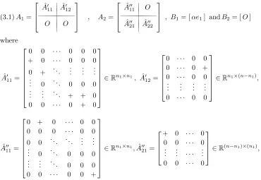
Let us consider annth order positive 2-D system (A1, A2, B1, B2) withn≥n1≥
3,B2=O, whereOis the zero matrix of an appropriate size,B1= [αe1] withα >0
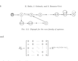
(that is, a 1-monomial column vector) and 2-D influence digraph given in Fig. 3.2
where the verticesv1, v2, . . . , vn have been relabeled as the subindices 1, 2, . . . , nto
simplify. The preceding replacement is also carried out throughout this paper.
Therefore, the matrices of the system (A1, A2, B1, B2) are given as follows:
A1=
ˆ
A′ 11 Aˆ′12
O O
, A2=
ˆ A′′ 11 O ˆ A′′ 21 Aˆ′′22
, B1= [αe1] andB2= [O]
(3.1) where ˆ A′ 11=
0 0 · · · 0 0 0 + 0 · · · 0 0 0
0 + . .. ... ... ...
..
. 0 . .. 0 0 0
..
. ... . .. + + 0
0 0 · · · 0 + 0
∈Rn1×n1, Aˆ′ 12=
0 · · · 0 0 0 · · · 0 + 0 · · · 0 0
..
. ... ... ...
0 · · · 0 0
∈Rn1×(n−n1),
ˆ A′′ 11=
0 + 0 · · · 0 0 0 0 0 · · · 0 0
0 0 . .. ... ... ...
..
. 0 . .. 0 0 0
..
. ... . .. 0 0 0
0 0 · · · 0 0 +
∈Rn1×n1,Aˆ′′ 21=
+ 0 · · · 0 0 0 · · · 0 ..
. ... · · · ... 0 0 · · · 0
s 1 2 n1-2 n1-1 n1
n n
1+1 n1+2
[image:6.612.72.404.59.321.2]3
Fig. 3.2.Digraph for the new family of systems.
and
ˆ
A′′ 22=
0 0 · · · 0 0 + 0 · · · 0 0
0 + . .. ... ...
..
. . .. ... 0 ...
0 · · · 0 + 0
∈R(n−n1)×(n−n1),
+ denoting a strictly positive entry.
Notice that we may consider for the sake of simplicity all strictly positive entries equal to one. Furthermore, it is worth pointing out that we may assume that the digraph for this family of systems is reduced to be the digraph given in Fig. 3.3 in
the casen=n1. Then, we observe that the matrices of the system given in example
3.1 are structured as those seen above for n = 3 and n1 = 3. It is convenient to
establish now two preliminary technical lemmas in order to get an expression of the local reachability index for this class of systems.
s 1 2 3 n-2 n-1 n
Fig. 3.3.Digraph for the new family of systems in the casen=n1.
Preliminarily, to simplify notation, we define the paths (see Fig. 3.2) P0 ≡
{s −→ 1}, Pk
1 ≡ {1 −→ 2 −→ · · · −→ k} for 2 ≤ k ≤ n1−1, P1 = P1n1−1,
P2j≡ {1(n1+1)· · ·j}forn1+1≤j≤n,P2=P2n,P3≡ {n−→21}
and P4 ≡ {(n1−1) −→ n1} whose compositions are (1,0), (k−1,0), (n1−2,0),
(0, j−n1), (0, n−n1), (1,1) and (1,0) respectively. In the same way, we define the
cycles C1 ≡ {1 −→ 2 1}, C2 ≡ {(n1−1) −→ (n1−1)}, C3 ≡ {n1 n1} and
C4=P2⊔ P3with respective compositions (1,1), (1,0), (0,1) and (1, n−n1+ 1).
then there is at least ans-path of composition (p+λ, q+δ) terminating at a vertex belonging toV \ {n1} for everyλandδ∈Z+ such that 0≤δ≤n−n1+λ.
Proof. Firstly, assuming that we have ans-path P of composition (p, q) ending
in vertex 1, then the cycleC1 allows us to affirm that for allη∈Z+ there is also an
s-path of composition (p+η, q+η) terminating at vertex 1 since this cycle adds (η, η)
to the composition of the initial path after doingη laps.
Combining these s-paths P ⊔ηC1 with both the paths P1k for 2 ≤ k ≤ n1−1
and the path P1 and the cycle C2, it is immediately seen that for all α ∈ Z+ we
can find s-paths of composition (p+η +α, q+η) ending in a vertex belonging to
V1={1,2,3, . . . , n1−1}. Thus, takingλ=η+αandδ=η, it is inferred that there
ares-paths of composition (p+λ, q+δ) terminating at a vertex belonging toV1 for
everyλ∈Z+ and 0≤δ≤λ.
Consequently, if n1 = n ≥ 3, then the assertion of this theorem is established
because, in this case, the inequality 0≤δ≤n−n1+λis reduced to 0≤δ≤λand
V \ {n1}=V1.
Secondly, ifn > n1≥3, the pathsP2j,n1+ 1≤j≤n, allow us to claim that for
allβ∈Z+satisfying 1≤β≤n−n1there is ans-path of composition (p+η, q+η+β)
terminating at a vertex belonging toV2={n1+ 1, n1+ 2, . . . , n}. Choosingλ=ηand
δ=η+β, we have ans-path of composition (p+λ, q+δ) ending in a vertex belonging
toV2 for allλ, δ∈Z+ withλ+ 1≤δ≤n−n1+λ. Hence, sinceV \ {n1}=V1∪V2
the statement of this lemma is easily derived from.
Remark 3.3. In the event that n > n1, we stress that for a fixed valuep∈N
thes-paths consisting exactly ofp1-arcs which terminate at vertex 1 are only those
equal toP0⊔αC1⊔βC4withα+β+ 1 =p(except for some other rearrangements of
the same cycles, for instance,P0⊔ C4⊔ C1⊔(β−1)C4⊔(α−1)C1). With respect to
their lengths, the longest path is clearlyP0⊔(p−1)C4. Then,P0⊔(p−1)C4⊔ P2 is
the greatest in length among thoses-paths consisting precisely ofp1-arcs which end
in a vertex belonging toV \ {n1} and this vertex isn.
Analogously, P0⊔(p−1)C1 is the longest s-path among those of composition
consisting precisely ofp1-arcs which terminate atV\ {n1}, namely at vertex 1, when
n=n1.
Lemma 3.4. Letpbe any natural number, then there is ans-path of composition (p, β), β ∈ Z+, ending in a vertex belonging to V \ {n1} if and only if 0 ≤ β <
(n−n1+1)p. Besides that, there is a uniques-path of composition(p,(n−n1+1)p−1)
terminating at a vertex belonging toV \ {n1}.
enables us to assert that we can find s-paths of composition (1, β) with 0 ≤ β <
n−n1−1 ending in a vertex ofV \ {n1}because the pathP0terminates at vertex 1
and has composition (1,0). Conversely, according to the 2-D influence digraph given
in Fig. 3.2, thes-paths of composition (1, β) are onlyP0(withβ= 0) andP0⊔ P2n1+β
where 1≤β ≤n−n1. We observe that each of them ends in a vertex belonging to
V \ {n1}and in addition, forβ=n−n1, the correspondings-path is exactlyP0⊔ P2
whose final vertex isn. Hence, the assertion of this lemma forp= 1 is proven.
Let us assume that the same statement holds forp=α, that is,
• There exist s-paths of composition (α, β) ending in a vertex of V \ {n1} if
and only if
0≤β <(n−n1+ 1)α.
(3.2)
• There is a unique s-path of composition (α,(n−n1+ 1)α−1) ending in a
vertex belonging toV\{n1}. In fact, thiss-path is preciselyP0⊔(α−1)C4⊔P2
which terminates at vertexn.
Let us take now the case in whichp=α+ 1. We know that for everyt∈Nthere
exists-pathsP0⊔(t−1)C4of composition (t,(t−1)(n−n1+ 1)) terminating at vertex
1. In particular for eacht ∈ Nsatisfying 1 ≤t ≤α+ 1, we can apply successively
Lemma 3.2 to each one of these paths, taking p = t, q = (t−1)(n−n1+ 1) and
settingλ=α+ 1−t, that is, such thatp+λ=α+ 1. Hence, we can find at least an
s-path of composition (α+ 1, β) ending in a vertex ofV \ {n1}for eachβ∈Z+ such
thatq≤β≤q+n−n1+λ, so:
(t−1)(n−n1+ 1)≤β≤t(n−n1+ 1) +α−t .
(3.3)
Plugging the different values oftinto equation (3.3), we can assure that there is
at least an s-path of composition (α+ 1, β) for each 0 ≤β < (n−n1+ 1)(α+ 1)
terminating at a vertex belonging toV \ {n1}.
Let us suppose that there exists an s-path of composition (α+ 1, β) ending in
a vertex of V \ {n1} with β ≥ (n−n1+ 1)(α+ 1) and that such a vertex is v. If
v∈V1then we could construct ans-path of composition (α, β) for this sameβsimply
removing the last 1-arc of the initial path. This contradicts our inductive assumption.
Ifv∈V2 thenv=n1+kwherek∈ {1, . . . , n−n1}. Hence, the path constructed by
eliminating the lastk2-arcs of the starting path terminates at vertex 1. Moreover, it
has composition (α+ 1, β−k) withβ−k≥(n−n1+ 1)(α+ 1)−k > α(n−n1+ 1)
but this is impossible since P′ :=P
0⊔αC4 of composition (α+ 1, α(n−n1+ 1)) is
the longest among thoses-paths consisting ofα+ 1 1-arcs and ending in vertex 1 (see
We also conclude from remark 3.3 thatP′⊔ P
2 =P0⊔αC4⊔ P2 is the greatest
in length among those s-paths consisting exactly ofα+ 1 1-arcs which terminate at
vertexn. Thus, the proof is complete.
Case n = n1 ≥ 3: The same conclusion can be drawn for this situation, with
thes-pathsP0⊔(p−1)C4replaced by the s-pathsP0⊔(p−1)C1. It deserves to be
mentioned that the uniques-path of composition (α,(n−n1+ 1)α−1) = (α, α−1)
ends in vertex 1 instead of vertexn.
The following theorem provides us an expression of the reachability index for the specific class of systems we are considering in this paper.
Theorem 3.5. Let (A1, A2, B1, B2) be a positive 2-D system given as in (3.1).
Then, it is (positively) locally reachable and its local reachability index ILR is:
ILR=n1(n−n1+ 2).
(3.4)
Proof. Casen > n1≥3: Let us examine the deterministically reachable verticesv
and their corresponding determination indicesID(v). In particular, let us check that
every vertex is deterministically reachable and that ID(n1) provides the maximum
determination index, that is,ID(n1) =ILR.
We start by noting that we can find a unique path of composition (ℓ,0) ending in
ℓ, for allℓ∈V1={1, . . . , n1−1}. Then eachℓ,ℓ∈V1, is deterministically reachable
with composition (ℓ,0). In fact,
(A1ℓ−1⊔⊔0A2)B1= (A1ℓ−1⊔⊔0A2)αe1=βeℓ.
whereβ >0.
Likewise, every vertexℓwithℓ∈V2={n1+ 1, . . . , n} is deterministically
reach-able with composition (1, ℓ−n1) since
(A10⊔⊔ℓ−n1A2)B1= (A10⊔⊔ℓ−n1A2)αe1=γeℓ.
whereγ >0. That is, there exists a unique path of composition (1, ℓ−n1) terminating
atℓ, for allℓ∈V2. Hence, obviously
ID(1) = 1, ID(2) = 2, . . . , ID(n1−1) =n1−1,
ID(n1+ 1) = 2, ID(n1+ 2) = 3, . . . , ID(n) =n−n1+ 1.
(3.5)
Therefore, to complete the local reachability analysis of this system, it is necessary
to analyze whether the vertex n1 is deterministically reachable or not as well as
we must calculate the shortest length among thoses-paths of 2-D influence digraph
deterministically reachingn1.
In order to obtain an s-path ending in vertex n1, we emphasize that an s-path
may end in vertexn1 only if it contains at least n1 1-arcs. Notice that the s-path
P0⊔P1⊔P4of composition (n1,0) terminates at vertexn1. Furthermore, in accordance
with Lemma 3.4, there is an s-path of composition (n1+λ, β) ending in V \ {n1}
if and only if 0 ≤ β < (n1+λ)(n−n1+ 1). Hence, if there exists an s-path of
composition (n1+λ, β) withβ ≥(n1+λ)(n−n1+ 1), then this one can terminate
uniquely at vertex n1. Note that it is straightforward that if there is an s-path of
composition (n1, n1(n−n1+ 1)) then it is the shortest among those s-paths of the
2-D influence digraph deterministically reachingn1. Such ans-path of composition
(n1, n1(n−n1+ 1)) deterministically reachingn1isP0⊔ P1⊔ P4⊔(n1(n−n1+ 1))C3.
Thus,ID(n1) =n1+ (n−n1+ 1)n1=n1(n−n1+ 2). Consequently, all vertices are
deterministically reachable and the system is locally reachable. It is obvious that the
determination indexID(n1) is greater than the determination indices found in (3.5).
Hence,
ILR =ID(n1) =n1+n1(n−n1+ 1) =n1(n−n1+ 2),
which completes the proof.
Case n=n1≥3: The details are left to the reader since similar considerations
as formerly indicated show that
ID(1) = 1, ID(2) = 2, . . . , ID(n−1) =n−1, ID(n) =ID(n1) = 2n.
and hence the theorem follows.
From this result we conclude:
Corollary 3.6. The maximum local reachability index ILR for a positive 2-D
system given as in(3.1)for a natural number n1 is attained at
n1= n
2 + 1 ifn is an even natural number and
n1= n+ 1
2 or
n+ 3
2 ifn is an odd natural number. (3.6)
Hence, the maximumILR is achieved for those systems satisfying n1=n2+ 1and
can be written uniformly like:
ILR =
n
2
+ 1 n+ 1−n
2
.
(3.7)
Moreover,ILR is upper bounded by (n+2)
Proof. For a fixed natural numbern, we obtain that n1= (n+2)2 is the point of
maximum of the function ILR =ID(n1) =n1(n−n1+ 2), since its derivative with
respect ton1, dIDdn(n1)
1 , is positive forn1<(n+ 2)/2 and negative for n1>(n+ 2)/2.
Thus, if n is an even natural number then, n1 = (n+2)2 = n2 + 1 = n2+ 1, but
if n is an odd natural number then n1 cannot take the value (n+2)2 , since it is not
a natural number and in this case, we deduce that the vertex n1 has to be n+12 =
n
2
+ 1 or n+3
2 =
n
2
+ 2, studying the closest natural values in this parabola to the
aforementioned one corresponding ton1which is the desired initial assertion. In fact,
ID(
n+ 1
2 ) =
n+ 1
2 (n−
n+ 1
2 + 2) = (n+ 1)
2
(n+ 3)
2 =
n+ 3
2 (n−
n+ 3
2 + 2) =ID( n+ 3
2 ).
In addition, it is clear that ifnis an even natural number, an upper bound onILR
given in expression (3.7) is (n+2)4 2. In the same way, if nis an odd natural number,
an upper bound on ILR given in expression (3.7) is (n+1)(4n+3). HenceILR≤ (n+2)
2 4
since (n+ 2)2= (n+ 1)(n+ 3) + 1 which proves this corollary.
Dimension n 4 5 6 7 10 11 15 20
ILR
n
2
+ 1 n+ 1−n
2
9 12 16 20 36 42 72 121
Table 3.1
Minimum values corresponding to the upper bounds onILRfor any positive2-D system.
Remark 3.7. As a consequence of the preceding corollary, we can state that an
upper bound onILR for any (positively) locally reachable 2-D system must be greater
than or equal to (n+2)4 2.
The study of an upper bound on the whole is still an open problem.
Acknowledgments. We wish to express our gratitude to the reviewers for the several helpful comments which have allowed us to improve the clarity of this paper.
REFERENCES
[1] E. Bailo , J. Gelo nch, and S. Ro mero -Viv´o. ´Indice de alcanzabilidad: Sistemas 2D positivos con 2 ciclos (In Spanish).Proceedings of XX CEDYA-X CMA, Sevilla (Spain), 2007. [2] E. Bailo, J. Gelonch, and S. Romero. Additional results on the reachability index of positive
2-D systems.Lecture Notes in Control and Information Sciences, 341:73–80, 2006. [3] E. Bailo, R. Bru, J. Gelonch, and S. Romero. On the reachability index of positive 2-D systems.
IEEE Trans. Circuits Syst. II: Express Brief, 53(10):997–1001, 2006.
[4] R. Bru, L. Cacceta, and V. G. Rumchev. Monomial subdigraphs of reachable and controllable positive discrete-time Systems.Int. J. Appl. Math. Comput. Sci., 15(1):159–166, 2005. [5] R. Bru, C. Coll, S. Romero, and E. S´anchez. Reachability indices of positive linear systems.
[6] R. Bru, C. Coll, S. Romero and E. S´anchez. Some problems about structural properties of positive descriptor systems.Lecture Notes in Control and Information Sciences, 294:233– 240, 2004.
[7] R. Bru, S. Ro mero , and E. S´anchez. Canonical forms of reachability and controllability of positive discrete-time control systems.Linear Algebra Appl., 310:49–71, 2000.
[8] R. Bru, S. Ro mero -Viv´o, and E. S´anchez. Reachability indices of periodic posi-tive systems via posiposi-tive shift-similarity. Linear Algebra Appl., 429(1): 1288–1301, doi:10.1016/j.laa.2008.01.033, 2008.
[9] P. Brunovsky. A classification of linear controllable systems.Kybernetika, 3(6):173–188, 1970. [10] C. Coll, M. Fullana, and E. S´anchez. Some invariants of discrete-time descriptor systems.Appl.
Math. on Computation, 127:277–287, 2002.
[11] C. Commault. A simple graph theoretic characterization of reachability for positive linear systems. Systems and Control Letters, 52(3-4):275–282, 2004.
[12] P. G. Coxson and H. Shapiro. Positive reachability and controllability of positive systems.
Linear Algebra Appl., 94:35–53, 1987.
[13] P. G. Coxson, L. C. Larson, and H. Schneider. Monomial patterns in the sequenceAkb .Linear Algebra Appl., 94:89–101, 1987.
[14] M. P. Fanti, B. Maione, and B. Turchiano. Controllability of linear single-input positive discrete time systems. International Journal of Control, 50:2523–2542, 1989.
[15] M. P. Fanti, B. Maione, and B. Turchiano. Controllability of multi-input positive discrete time systems. International Journal of Control, 51:1295–1308, 1990.
[16] E. Fornasini. A 2-D systems approach to river pollution modelling. Multdim. Syst. Signal Proc., 2(3):233–265, 1991.
[17] E. Fornasini and G. Marchesini. State-Space realization of two-dimensional filters. IEEE Transactions on Automatic Control, AC-21(4):484–491, 1976.
[18] E. Fornasini and M. E. Valcher. Controllability and Reachability of 2-D Positive Systems: A Graph Theoretic Approach.IEEE Trans. Circuits Syst. I: Regular Papers, 52(3):576–585, 2005.
[19] L.R. Foulds. Graph Theory Applications(2nd
edition). Springer Verlag, New York, 1995. [20] T. Kaczorek. Reachability and controllability of positive linear systems with state feedbacks.
Proceedings of the 7th Mediterranean Conference on Control and Automation (MED99), Haifa (Israel), 1999.
[21] T. Kaczorek. Reachability and controllability of 2D positive linear systems with state feedback.
Control and Cybernetics, 29(1):141–151, 2000.
[22] T. Kaczorek. Positive 1D and 2D Systems. Springer, London, United Kingdom, 2002. [23] T. Kaczorek. Reachability index of the positive 2D general models. Bull. Polish Acad. Sci.,
Tech. Sci., 52(1):79–81, 2004.
[24] T. Kaczorek. New reachability and observability tests for positive linear discrete-time systems.
Bull. Polish Acad. Sci., Tech. Sci., 55(1):19–21, 2007.
[25] W. Marszalek. Two-dimensional state space discrete models for hyperbolic partial differential equations Appl. Math. Model., 8(1):11–14, 1984.
[26] V. G. Rumchev and D. J. G. James, Controllability of positive linear discrete time systems.