Contact Geometry of Curves
⋆Peter J. VASSILIOU
Faculty of Information Sciences and Engineering, University of Canberra, 2601 Australia
E-mail: [email protected]
Received May 07, 2009, in final form October 16, 2009; Published online October 19, 2009 doi:10.3842/SIGMA.2009.098
Abstract. Cartan’s method of moving frames is briefly recalled in the context of immersed curves in the homogeneous space of a Lie group G. The contact geometry of curves in low dimensional equi-affine geometry is then made explicit. This delivers the complete set of invariant data which solves theG-equivalence problem via a straightforward procedure, and which is, in some sense a supplement to the equivariant method of Fels and Olver. Next, the contact geometry of curves in general Riemannian manifolds (M, g) is described. For the special case in which the isometries of (M, g) act transitively, it is shown that the contact geometry provides an explicit algorithmic construction of the differential invariants for curves in M. The inputs required for the construction consist only of the metric g
and a parametrisation of structure group SO(n); the group action is not required and no integration is involved. To illustrate the algorithm we explicitly construct complete sets of differential invariants for curves in the Poincar´e half-space H3
and in a family of constant curvature 3-metrics. It is conjectured that similar results are possible in other Cartan geometries.
Key words: moving frames; Goursat normal forms; curves; Riemannian manifolds
2000 Mathematics Subject Classification: 53A35; 53A55; 58A15; 58A20; 58A30
1
Introduction
The classical topic of immersed submanifolds in homogeneous spaces via rep`ere mobileor mo-ving frames is discussed here in the simplest case, that of curves. Several authors have written on the method of rep`ere mobile, over the years since Cartan’s works, such as [5]; these include S.S. Chern [6], J. Favard [8], P.A. Griffiths [12], G.R. Jensen [14], M.L. Green [11], R. Su-lanke [26], R. Sharpe [21] and M.E. Fels & P.J. Olver [9, 10]. Some of these authors have the goal of placing Cartan’s method on a firm theoretical foundation as well as extending its range of application beyond the classical realm. More recently, a reformulation of the method of moving frames, due to Fels and Olver [9,10] has lead to renewed activity and a great many new applications and perspectives, have arisen (see [18] and references therein). Whereas Car-tan emphasised the construction of canonical Pfaffian systems whose integral manifolds are the Frenet frames along the submanifold, a much more direct approach is favoured in the Fels–Olver formulation and this has a number of significant advantages. However, in this paper, we shall reconsider the role of Pfaffian systems in the method of moving frames in the light of recent results in the geometry of jet spaces with the principal goal of making the contact geometry of curves more explicit and giving some indication about its possible applications. Another goal is to provide additional insight into the relationship between Cartan’s method of moving frames and the equivariant method of Fels and Olver1.
⋆This paper is a contribution to the Special Issue “´Elie Cartan and Differential Geometry”. The full collection
is available athttp://www.emis.de/journals/SIGMA/Cartan.html
1A point we make herein is that the geometry of jet spaces provides a useful mediation between the two
The considerations in this paper were inspired by a paper of Shadwick and Sluis [20], in which the authors observed that many of the Pfaffian systems derived by Cartan admit a Cartan pro-longation which is locally diffeomorphic to the contact distribution on jet space Jk(R,Rq), for
somekandq, thereby explicitly adding contact geometry to Cartan’s method of moving frames. Another way to view the aims of this paper is the further development of the ideas in [20] in re-lation to moving frames for curves by exploring the application of a recent generalisation [27,28] of the Goursat normal form from the theory of exterior differential systems [25,3] allowing for the explicit determination of differential invariants and other invariant data in cases which have not been previously explored in detail. Of particular interest are curves in general Cartan geo-metries and in this paper we have focused on the Riemanniancase and conjecture that similar results hold for other Cartan geometries.
We show that given any n-dimensional Riemannian manifold (Mn, g) then the Pfaffian system whose integral manifolds determine the Frenet frames along curves in M has a Car-tan prolongation which can be identified with the contact system on jet space Jn(R,Rn−1).
The explicit construction of the identification requires only differentiation. In case the isome-tries of (Mn, g) act transitively then the construction of the differential invariants that
set-tles the equivalence problem for curves up to an isometry differs from the approach of Fels– Olver in that explicit a priori knowledge of the isometries or even the infinitesimal isometries is not required; as in the Fels–Olver method no integration is called for. The inputs for al-gorithm Riemannian curves consist only of the metric g and a realisation of the Lie group SO(n).
Moreover, a contention of this paper is that the contact geometry of submanifolds to be described belowshould bea fundamental fact and lead to useful points of view that complement and enhance the geometric analysis of submanifolds by existing methods such as Cartan’s method of moving frames and the equivariant moving frames method of Fels and Olver.
The content of this paper is as follows. After briefly recalling the method of moving frames, as practiced by Cartan, we study one of the simplest non-trivial examples: curves in 2-dimensional equi-affine geometry. It is then shown how the (classical) Goursat normal form applies to give the unique differential invariant and moving frame, explicitly. This familiar, illustrative example encapsulates the ideas proposed in this paper and is simple enough so that all de-tails can be given. An account of the generalised Goursat normal form [27, 28] is then given in the special case of total prolongations (uniform Goursat bundles) in preparation for the study of immersed curves in higher dimensional Cartan geometries. Section 4 illustrates the principles developed in the previous section by applying it to study curves in 3d-equi-affine geo-metry, computing the complete set of differential invariants via the generalised Goursat normal form.
Section 5 is devoted to the contact geometry of curves in any Riemannian manifold and contains the main application of the paper. The general method is used to explicitly derive the differential invariants for curves in the Poincar´e half-spaceH3 and for curves in a family of constant curvature 3-metrics. These invariants do not seem to have appeared in the literature before. The results demonstrate that the contact geometry of submanifolds can offer an alter-native path to invariant data for curves besides the Fels–Olver equivariant method and Cartan’s method which, in the latter case, relies so much on geometric insight and special tricks for the construction of the Frenet frames2.
Finally, it should be mentioned that while this paper only explores the case of curves, the contact geometry of higher dimensional submanifolds could be similarly studied, commencing with the well known characterisation of contact systems in any jet space given in [2,30].
2In Cartan’s writings the distinction between the Frenet frames along a submanifold and the exterior differential
2
Method of rep`
ere mobile applied to curves
According to [14] the general problem treated by Cartan in [5] and elsewhere is that of the
invariants of submanifolds in the homogeneous space of a Lie group G under the action of G. In this section, I will give a very brief description of the method of rep`ere mobile, Cartan’s principal tool for addressing this type of problem. More complete discussions can be found in the references quoted above such as [8,12,14,26]. The exposition given by Cartan in [4] is still well worth reading.
LetGbe a Lie group and H⊂Ga closed subgroup. Then we have theH-principal bundle
H ι //G
π
G/H
of left cosets ofH inGand we letM :=G/H. Mapπ is the natural projection assigning a left-cosetgHto each element ofg∈G. There is a natural left-action ofGonM: g·zH =gzH, for all g∈G. Letxbe a local coordinate system on M. Cartan typically began with a representation ofGwhich could be “decomposed” into columnse1, e2, . . . , er ofH⊂Gand x, a column vector
whose components are the coordinates x on M. Cartan defines differential 1-formsωi, 1≤i≤r by
dx=
r X
i=1
ωi⊗ei. (1)
The 1-forms ωi are semi-basic for π. Furthermore, we have 1-formsωj
i defined by
dei = r X
j=1
ωji ⊗ej. (2)
The 1-forms ωi,ωij, i, j= 1, . . . , rare the components of the Maurer–Cartan form ω on G; the integral submanifolds of the Pfaffian system
ω1 = 0, ω2 = 0, . . . , ωr= 0
foliatesG by the left cosets ofH.
Suppose f : T → M is an immersion of a manifold T into M. Then a moving frame is a local map F : T → G such that f = π ◦ F. That is, the moving frame assigns to each point t ∈ T a coset f(t) ∈ G/H. With this general set up, Cartan addresses the following problem for submanifolds of M. Let f1 : T1 → M and f2 : T2 → M be submanifolds. Find necessary and sufficient conditions, in the form of differential invariants, such that there is a local diffeomorphismµ:T1 →T2 and elementg∈Gsuch that
f2◦µ=g·f1.
The ‘◦’ denotes function composition while ‘·’ continues to denote the left-action of G on M. A special case of this is the so-calledfixed parametrisationproblem where one takesT1 =T2=T andµis the identity onT. Thiscongruence problemis the one that will be studied in this paper. In case the submanifolds ofM are curves, Cartan begins by choosing a codimension 1 subset of the semibasic 1-forms and defines the Pfaffian system
One studies the solutions of Ω since these project via π down to curves in G/H, which are the objects of interest. One way to do this is via the Cartan–K¨ahler theorem [3]. Accordingly, one computes the exterior derivatives of the ωj, j = 2, . . . , r and appends these “integrability conditions” to Ω forming the differential ideal ¯Ω with independence form ω1. This procedure allows one to prove existence of integral curves for Ω and provides information about the number of such integral curves. However, this makes no use of the special origin of the 1-forms in Ω, arising as they do from the Maurer–Cartan form ω on G. As a result of this one can go much further. From the structure equations of ω and the vanishing of the exterior derivativesdωi we
deduce additional 1-form equations of the form
ωij−pjiω1 = 0,
for some functionspji onG, which are appended to Ω as integrability conditions, thereby forming the new Pfaffian system
¯
Ω : ω2= 0, ω3 = 0, . . . , ωr= 0, ωij−pjiω1 = 0.
In essence, the method of moving frames consists of using the fact that H acts on the fibres of G → G/H on the right inducing a transformation of the Maurer–Cartan formω on G, [23, Chapter 7]. Indeed, the transformation
(x, e1, . . . , er)7→(x, e1, . . . , er)h, ∀h∈H (3)
on Ginduces the transformation
ω7→Ad(h−1)ω+h−1dh=ωe (4)
on the Maurer–Cartan form ω. In turn, this induces a transformation on the functions pji. To proceed further we recall the notion of a Cartan prolongation.
Definition 1. Let I be a Pfaffian system on manifold M and p : Mc → M a fibre bundle. A Pfaffian systemIb on Mcis said to be aCartan prolongation of (M,I) if
1) p∗I ⊆Ib;
2) for every integral submanifold σ : S → M of I there is a unique integral submanifold
b
σ :S→Mcof Ibthat projects to σ; that is, σ=p◦σ.b
We say that σb is theCartan liftof σ.
If we choose to view (G×Rs,Ω), where the factor¯ Rscarries the “parameters”pj
i, as a Cartan
prolongation of (G,Ω) then (3) induces a reduction of the trivial bundle G ×Rs → G by
normalising the coordinates pji on the fibres to simple constants like 0 and±1.
Once ¯Ω has been normalised, the process begins again by taking exterior derivatives of the enlarged, normalised Pfaffian system arising from ¯Ω. Each step selects a subgroup K ⊂H. If the process terminates atK ={identity}ofGthen the resulting Pfaffian system arising from ¯Ω is canonical. The integral submanifolds of ¯Ω are the Frenet frames,F. Hereafter we shall label this canonical Pfaffian system by the symbol ΩF.
The main assertion made in this paper is that the canonical Pfaffian system ΩFdetermining
each Frenet frame along an immersed curve admits a Cartan prolongation ΩbFon E :=G×Rν
for someν, so that (E,ΩbF) is locally diffeomorphic to a jet space (Jk(R,Rq),Ωk(R,Rq)) where
carry the differential invariants of the problem. Indeed, the integral manifolds of ΩbF, say,
where I ⊆R is an interval. Hereafter, one of our goals is to give examples which demonstrate
the assertion made above, namely that the Pfaffian systemΩbFcan be identified with a contact
system. This identification can be constructed explicitly and provides explicit coordinate for-mulas for all the invariant data: differential invariants, Fels–Olver equivariant moving frames and invariant differential forms. In Section 5 we will prove that this procedure can be applied to curves in any Riemannian manifold and in that case it is algorithmic3. Importantly, one is not required to explicitly know the group action a priori. Before this we will work out some pedagogical examples. The first of these is sufficiently low dimensional so that all details can be given.
2.1 Curves in the equi-af f ine plane
The goal in this subsection is to provide a simple illustration of the method of moving frames as described in the previous subsection. We will construct the Frenet frame F for a plane curve up to equi-affine transformations by constructing the canonical Pfaffian system ΩFand
the appropriate Cartan prolongation ΩbF, as described above. Here equi-affine transformations
means the standard transitive action of the Lie group G = SL(n,R)⋉ Rn on Rn. For plane
andad−bc= 1. We call this homogeneous space theaffine planeand denote it byA2. For local
coordinates on A2 we take x, the first column of g ∈ G and e1, e2 are the next two columns
3In this paper a construction or procedure is said to bealgorithmicif it can be performed only by differentiation
where β = (1 +bc)/a, where we have chosen a chart on SL(2,R) in which a 6= 0; note that
ω1
1 +ω22 = 0. It is useful to record the structure equations
dω1 =ω1∧ω11+ω2∧ω12,
dω2 =ω1∧ω12−ω2∧ω11,
dω11 =ω21∧ω12, (6)
dω12 =−2ω11∧ω12, dω21 = 2ω11∧ω21.
Successive adapted frames are integral curves of certain Pfaffian systems which will be denoted by Ωi,i= 1,2, . . .. The first adapted frames for curves inA2 are integral curves of the Pfaffian system Ω1, consisting of the single 1-form equation
Ω1 : ω2 = 0
with independence form ω1. From structure equations (6), we obtain 0 = dω2 ≡ ω1 ∧ω2 1 mod ω2 and hence to complete Ω1 to a differential ideal ¯Ω1 we extend it by appending the 2-form equation ω21∧ω1 = 0. This equation implies that there is a function p on G such that the 2-form equation can be replaced by ω2
1−p ω1 = 0, a kind of “first integral”. We extend Ω1 by this 1-form equation and rename the extended Pfaffian system ¯Ω1 to get
¯
Ω1 : ω2 = 0, ω12−p ω1= 0.
Note that the reconstituted ¯Ω1 is no longer a differential ideal.
As discussed in Section 2, an element h ∈ H acts on the frame [x, e1, e2] over each point x ∈ G/H on the right inducing the transformation (4) on the Maurer–Cartan form on G. This, in turn induces a transformation on the function p. The subgroup H1 ⊂ H that leaves Ω1-invariant has representation
1 0 0
0 a b
0 0 1/a
.
We obtain
e
ω1 =a−1ω1, ωe2 =aω2, eω21 =a2ω12.
Hence
0 =ω12−p ω1=a−2ωe21−p aωe1 =a−2(ωe12−p a3ωe1).
The Pfaffian system ¯Ω1 is transformed to
e
ω2 = 0, ωe12−p a3eω1 = 0.
That is, the function pundergoes the transformationp7→a3p. Accordingly, we can chooseaso that ap3= 1 and transform ¯Ω1 to4
Ω2 : ω2 = 0, ω12−ω1 = 0.
4We have made a tacit genericity assumption thatp6= 0. The casep= 0 must be considered separately, as
The integral submanifolds of Ω2, with independence form ω1 are the “second order frames” for curves inA2. The subgroup H2⊂H1 ⊂H that preserves the elements of Ω2 is
1 0 00 1 b 0 0 1
.
We must now extend Ω2 to a differential ideal by computing the exterior derivative ofω2 1−ω1. From the structure equations we obtain 3ω11∧ω1 = 0. As before, there is a functionqonGsuch that the 2-form equation can be replaced by
ω11−qω1= 0
so that (the reconstituted) ¯Ω2 is given by the 1-form equations
¯
Ω2 : ω2 = 0, ω12−ω1 = 0, ω11−qω1= 0 (7)
and is no longer a differential ideal.
By performing aH2 change of frame the 1-forms in (7) become
e
ω2 =ω2, ωe12−eω1 =ω12−ω1, ωe11=ω11−b ω21.
Thus Ω2 is invariant under aH
2 change of frame while
0 =ω11−qω1=ωe11+ (b−q)ωe1.
We can chose b=q to obtain the 1-form equation eω11 = 0, and giving rise to the final adapted frame (dropping tildes)
Ω3 : ω2 = 0, ω12−ω1 = 0, ω11 = 0
which “reduces the isotropy group to the identity”. Thus, Ω3 is the Pfaffian system Ω
F and
its integral curves are the Frenet lifts F of curves in A2. Computing the exterior derivative of
ω11 = 0 we obtain the 2-form equation ω12∧ω1 = 0 and hence there is a function κ on G such thatω1
2−κω1 = 0. This time there is no freedom left in our choice of frame that enablesκto be transformed away. The functionκhere is intrinsic. Hence, in this case, the Cartan prolongation we seek is the Pfaffian system ΩFaugmented by the 1-form equationω12−κω1 = 0
b
ΩF: ω2 = 0, ω21−ω1 = 0, ω11 = 0, ω12−κω1= 0,
on G×Rκ. The integral curves of ΩbFwith independence form ω1 determine the unique
equi-affine invariant for plane curves.
Theorem 1. LetI ⊆Rbe an interval and γi :I →A2 be two immersed curves in the equi-affine
plane, each parametrised by equi-affine arc-length. Then there is an element g ∈ G such that
γ2=g·γ1 if and only if their Cartan lifts Γbi:I →G×R satisfy
b
Γ∗1κ=bΓ∗2κ (8)
identically on I.
Proof . Let us firstly recall that (G×R,ΩbF) → (G,ΩF) is a Cartan prolongation and Γbi is
andbΓiare Cartan lifts ofγi. FinallyΓbi are integral submanifolds ofΩbFonG×Rand consquently
fori= 1,2 we have
b
Γ∗iω2 =Γb∗iω11 = 0, Γb∗iω12 = bΓi∗κ bΓ∗iω1, Γbi∗ω21 =Γb∗iω1. (9)
Since both curves are parametrised by equi-affine arc-length swe have bΓ∗1ω1 =Γb∗2ω1 = ds. From this and from (9) we deduce that
Γ∗1ΩMC= Γ∗2ΩMC, (10)
where ΩMCis the Maurer–Cartan form onG. It follows from the standard theorem about maps into a Lie group [22, Chapter 10, Theorem 18] that there is a fixed element g ∈ G such that γ2=g·γ1.
Conversely, if γ2 = g·γ1 for some g ∈ G, then the Frenet lifts Γi of γi satisfy (10) and
are integral submanifolds of ΩF. But since ΩbF is a Cartan prolongation of ΩF, there are
Car-tan lifts bΓi of Γi which are integral submanifolds of ΩbF. Equation (8) follows from this and
equation (10).
Remark 1. This theorem encapsulates the basic idea of this paper and is proposed as a model for the study of curves in any Cartan geometry. The relationship between Theorem 1 and diagram (5) should be clear. The idea now is that by the Goursat normal form G×R,Ωb⊥
F
is locally diffeomorphic to the jet bundle J4(R,R),C(4)
1
, whereC1(4) is the contact sub-bundle of T J4(R,R). That is, there is a local diffeomorphismφ:G×R→J4(R,R) such thatφ
∗Ωb⊥F =C
(4) 1 . In fact, Theorem 1 proves that knowing the diffeomorphismφexplicitly constructs the unique invariant κ for plane equi-affine curves explicitly, namely the equi-affine curvature, as well as the equi-affine arc-length. Explaining this is the goal of the next subsection.
2.2 Goursat normal form
The Goursat normal form is a local characterisation of the contact distribution on Jk(R,R)
for all k ≥ 1, which we denote C(1k). The original theorem is not due to Goursat who was its populariser. It appears the theorem is originally due, in some form, to E. von Weber but the statement of it I give below essentially arises from a 1914 work of Cartan. A good reference is [25]. This reference describes an interesting, relevant but largely forgotten work of Vessiot [29]. First we establish some notation and definitions.
2.2.1 The derived f lag
SupposeM is a smooth manifold andV ⊂T M a smooth sub-bundle of its tangent bundle. The structure tensor is the homomorphism of vector bundles δ: Λ2V →T M/V defined by
δ(X, Y) = [X, Y] mod V, for X, Y ∈Γ(M,V).
If δ has constant rank, we define the first derived bundle V(1) as the inverse image of δ(Λ2V) under the canonical projectionT M →T M/V. Informally,
V(1)=V+ [V,V].
The derived bundlesV(i) are defined inductively:
assuming that at each iteration it defines a vector bundle, in which case we shall say that V is
regular. For regularV, by dimension reasons, there will be a smallestkfor whichV(k+1) =V(k). This kis called thederived length of V and the whole sequence of sub-bundles
V ⊂ V(1)⊂ V(2)⊂ · · · ⊂ V(k)
thederived flag ofV. We shall denote byV(∞) the smallest integrable sub-bundle containing V.
2.2.2 Cauchy bundles
Let us define
σ : V →Hom(V, T M/V) by σ(X)(Y) =δ(X, Y)
Even if V is regular, the homomorphism σ need not have constant rank. If it does, let us write Char V for its kernel. The Jacobi identity shows that CharV is always integrable. It is called the Cauchy bundle or characteristic bundle of V. If V is regular and each V(i) has a Cauchy bundle then, we say that V istotally regular. Then by the derived typeof V we shall mean the list {V(i),CharV(i)}of subundles.
Theorem 2 (Goursat normal form). Let V ⊂ T M be a smooth, totally regular, rank 2
sub-bundle over smooth manifold M such that
a) V(∞)=T M;
b) dimV(i+1)= dimV(i)+ 1, while V(i) 6=T M.
Then there is a generic subsetMˆ ⊆M such that in a neigbourhood of each point of Mˆ there are local coordinates x, z0, z1, z2, . . . zk such that V has local expression
(
∂x+ k X
j=1
zj∂zj−1, ∂zk
)
,
where k= dimM −2. That is, V is locally equivalent to C1(k) on Mˆ.
A proof can be found in [25, pp. 157–159]. The proof of a much more general result in which the Goursat normal form is a special case is given in [28]. The significance of the latter is that an procedure is provided for constructing the local contact coordinates x, z0, . . . , zk. This is
procedureContact B on page 287 of [28] with ρk = 1 and ρ1 =ρ2 =· · ·=ρk−1 = 0; theρi are
defined in Section 3. In this special case we have the following.
Procedure Contact for the Goursat normal form
INPUT: Sub-bundle V ⊂ T M of derived length k which satisfies the hypotheses of Theorem2.
a) Fix any first integral of CharV(k−1), denotedx, and any sectionZofV such thatZx= 1.
b) Define a distribution Πk as follows:
Πl+1 = [Z,Πl], Π1 = CharV(1), 1≤l≤k−1.
c) Letz0 be any invariant of Πk such thatdx∧dz0 6= 0. d) Define functionsz1, z2, . . . , zk by zj =Zzj−1,j= 1, . . . , k.
OUTPUT: Functions x, z0, z1, . . . , zk are contact coordinates forV.
2.3 Equi-af f ine invariants & the Goursat normal form
We use this procedure to construct the various invariant objects for this geometry. In fact we will construct the Frenet frames by constructing all the integral submanifolds of ΩbF. So we set
V :=Ωb⊥
F:
V =∂ω1 +∂ω2
1 +κ∂ω12, ∂κ .
Note that we have adopted the usual convention of denoting the frame dual to
ω1, ω2, ω11, ω12, ω21
Calculation verifies that the hypotheses of Theorem 2are met and that the derived length ofV is k= 4. Then step a) of Contactrequires that we construct at least one invariant of
CharV(3) =∂b, ∂κ, a∂a+c∂c
which has invariants x, y, a/c. Any one of these can be taken as the “independent variable”. Sincex, yare local coordinates onG/SL(2,R), we shall choosexfor this purpose. It then follows
that we may take Z to be
Step b) requires the construction of Π4. We get
Hence if we express the curve in A2 as a graph (x, f(x)) then we deduce from φ−1 that the
equi-affine curvature is the well known expression
κ:= 5f
′′′(x)2−3f′′(x)f′′′′(x)
9f′′(x)8/3 = 1 2 f
′′(x)−2/3′′ .
We also obtain the unique G-invariant 1-form, the equi-affine arc length by pulling back ω1 by φ−1,
(φ−1)∗ω1 =f′′(x)1/3dx
and the Frenet frame
F=
1 0 0
x f′′(x)−1/3 −3−1f′′′(x)f′′(x)−5/3
f(x) f′(x)f′′(x)−1/3 (f′′(x)2−3−1f′′′(x)f′(x))f′′(x)−5/3
of the curve (x, f(x)) by pulling back an arbitrary element g ∈ G by φ−1. Of course, we can express everything in terms an arbitrary immersion (x(t), y(t)) intoA2, rather than as a graph.
Remark 2. Note that the procedure we have just described for the invariant data of curves in A2 is not algorithmic; we had to solve differential equations to obtain the equivalence φ. In
practice, however, we find that when the contact system is that of Jk(R,Rq) whereq > 1, this
integration can often be avoided. We will illustrate this for curves inA3 and prove, in Section5,
that it holds for curves in any Riemannian manifold of dimension greater than 2.
3
On the generalised Goursat normal form
To carry out the programme of the previous section for curves immersed in manifolds of dimen-sion greater than two we must be able to characterise the contact distributions on jet spaces Jk(R,Rq), for all k, q ≥ 1; the case q = 1 being the Goursat normal form. In principle this
generalisation should include partial prolongations of the contact distribution on J1(R,Rq) and
such a characterisation exists – the generalised Goursat normal form [27, 28]. However, so far the full scope of this characterisation has not been required. It turns out that onlytotal prolon-gations of the first order jet space are sufficient. Accordingly, we will only briefly review those parts of [27,28] that are needed for the results to be described in this paper.
3.1 The singular variety
For eachx∈M, let
Sx ={v∈ Vx\0|σ(v) has less than generic rank}.
Then Sx is the zero set of homogeneous polynomials and so defines a subvariety of the
pro-jectivisation PVx of Vx. We shall denote by Sing(V) the fibre bundle over M with fibre over
x∈M equal toSx and we refer to it as the singular variety ofV. ForX∈ V the matrix of the
homomorphismσ(X) will be called thepolar matrixof [X]∈PV. There is a map deg
V :PV →N well defined by
degV([X]) = rank σ(X) for [X]∈PV.
a diffeomorphism φ:M1 →M2 that identifies them, then Sing(V2) and Sing(φ∗V1) are equiva-lent as projective subvarieties of PV2. That is, for each x ∈ M1, there is an element of the
projective linear group P GL(V2|φ(x),R) that identifies Sing(V2)(φ(x)) and Sing(φ∗V1)(φ(x)). We hasten to point out that the computation of the singular variety for any given sub-bundleV ⊂T M is algorithmic. One computes the determinantal variety of the polar matrix for generic [X].
3.1.1 The singular variety in positive degree
IfX∈CharV then degV([X]) = 0. It is convenient to eliminate lines of degree zero and for this reason we pass to the quotient Vb := V/CharV. We have structure tensor δb: Λ2V →b T M /d V,b well defined by
b
δ(X,b Yb) =π([X, Y]) mod V,b
where T Md =T M/CharV and
π : T M →T Md
is the canonical projection. The notion of degree descends to this quotient giving a map
degVb : PV →b N
well defined by
degVb([X]) = rankb bσ(X)b for [X]b ∈PVb,
where bσ(X)(b Yb) =δ(bX,b Yb) forYb ∈V. Note that all definitions go overb mutatis mutandis when the structure tensor δ is replaced by bδ. In particular, we have notions of polar matrix and singular variety, as before. However, if the singular variety of Vb is not empty, then each point of PVb has degree one or more.
3.1.2 The resolvent bundle
SupposeV ⊂T M is totally regular of rankc+q+ 1,q≥2,c≥0, dimM =c+ 2q+ 1. Suppose further that V satisfies
a) dim Char V =c,V(1)=T M;
b) Σb|x := Sing(V)b |x =PBb|x ≈ RPq−1, for each x ∈ M and some rank q sub-bundle B ⊂b V.b
Then we call (V,PB) (or (V,b Σ)) ab Weber structure of rankq on M.
Given a Weber structure (V,PB), letb R(V)⊂ V, denote the largest sub-bundle such that
π R(V)=B.b (11)
We call the rank q +c bundle R(V) defined by (11) the resolvent bundle associated to the Weber structure (V,Σ). The bundleb Bbdetermined by the singular variety ofVbwill be called the
singular sub-bundle of the Weber structure. A Weber structure will be said to beintegrable if its resolvent bundle is integrable.
An integrable Weber structure descends to the quotient of M by the leaves of Char V to be the contact bundle on J1(R,Rq). Thus, the resolvent bundle and its concomitant Weber
structure is a constructive characterisation of the contact bundle on the 1-jets J1(R,Rq). The
term ‘Weber structure’ honours Eduard von Weber (1870–1934) who was the first to publish a proof of the Goursat normal form. For completeness we record the following properties of the resolvent bundle of a Weber structure.
Proposition 1 ([27]). Let (V,Σ)b be a Weber structure onM andBbits singular sub-bundle. If
q ≥3, then the following are equivalent
a) its resolvent bundle R(V)⊂ V is integrable;
b) each point of Σ = Sing(b V)b has degree one;
c) the structure tensor δbof Vb vanishes onBb: bδ(B,b B) = 0b .
Proposition 2 ([27]). Let (V,Σ)b be an integrable Weber structure on M. Then its resolvent bundle R(V) is the unique, maximal, integrable sub-bundle of V.
Checking the integrability of the resolvent bundle is algorithmic. One computes the singular variety Sing(V) =b PB. In turn, the singular bundleb Bbalgorithmically determinesR(V).
Example 1. The canonical model of an integrable Weber structure is the contact distribution on J1(R,Rq) for q >1, extended by Cauchy characteristics
V =
(
∂x+ q X
i=1
pi∂ui, ∂p1, . . . , ∂pq, ∂z1, ∂z2, . . . , ∂zc
)
.
The quotientVb=V/CharV has singular sub-bundle
b
B=[∂p1], . . . ,
∂pq
and the resolvent bundle of integrable Weber structure (V,PB) isb
R(V) =∂p1, . . . , ∂pq, ∂z1, ∂z2, . . . , ∂zc .
The invariants of the resolvent bundle are spanned by{x, u1, . . . , uq}. So the resolvent bundle
provides a geometric characterisation of the “independent variable”xand the “dependent variab-les” ui, after which differentiation by a canonically defined total derivative operator leads to
higher order jet coordinates. See Sections3.2and4of this paper for further details. See [27,28] for the general theory with proofs and further examples.
3.2 The uniform generalised Goursat normal form
We are now able to give a characterisation of the contact distribution onJk(R,Rq),Cq(k) for any
k, q≥1, generalising the Goursat normal form to the uniform case.
Theorem 3 (generalised Goursat normal form – uniform case, [27, 28]). Let V ⊂T M
be a smooth, totally regular, sub-bundle of rank q+ 1 and derived lengthk, some k, q >0, over smooth manifold M such that
a) V(∞)=T M;
b) dimV(i+1)= dimV(i)+q, whileV(i)6=T M;
c) Char V(i)⊂ V(i−1), 1≤i≤k−1; dim CharV(j)=jq, 0≤j≤k−1; d) If q >1 thenV(k−1) admits an integrable Weber structure.
Then there is a generic subsetMˆ ⊆M such that around each point of Mˆ the distribution V
If q = 1 then c) follows from b) and the Weber structure is not defined in which case Theorem 3 reduces to the Goursat normal form, Theorem 2. We call any sub-bundle that satisfies the hypotheses of Theorem 3 a uniform Goursat bundle in which case the Theorem asserts that generically every uniform Goursat bundle is locally equivalent to the canonical one. A proof of Theorem3can be found in [27] as a special case of that paper’s Theorem 4.1. However, the latter covers a very much larger class of sub-bundles than uniform Goursat bundles and there is therefore a much simpler proof in this uniform case. However, for the purposes of this paper an important thing is the procedure for constructing contact coordinates in the uniform case which is a special case of procedure Contact A on page 286 of [28]5 with ρ1 = ρ2 = · · · =ρk=1 = 0, ρk=q >1. Note that the collection of non-negative integers
σ =hρ1, ρ2, . . . , ρki
shall be called the signature of V and is a complete local invariant of Goursat bundles. In the interests of completeness we mention that the non-negative integersρi are defined by
ρj = dim CharV(j)−dim CharVj(−1j) , 1≤j≤k−1,
ρk= dimV(k)−dimV(k−1),
where CharVj(j−1) = CharV(j)∩V(j−1). It is proved in [27,28] that a sub-bundleVon manifoldM is locally diffeomorphic to a partial prolongation of the contact systemCq(1) onJ1(R,Rq) withρj
variables of order j, if and only if (M, V) is a Goursat bundle of signatureσ. In this paper, we need only consider total prolongations in which the only nonzero element of the signature isρk,
where kis the derived length of V.
Procedure Contact for uniform generalised Goursat bundles, q >1
INPUT: Uniform Goursat bundleV ⊂T M of derived lengthk withq >1.
a) Construct the (integrable) resolvent bundle R(V(k−1)) and all its q+ 1 first integrals. b) Fix any one of the first integrals from step a) denotedx, and any sectionZofV such that
Zx= 1.
c) Denote the remaining q first integrals ofR(V(k−1)) byzj
0,j= 1,2, . . . , q.
d) Define functionszj1, z2j, . . . , zkj by zjm=Zzmj−1, 1≤m≤k, 1≤j≤q.
OUTPUT: Functions x, z0j, z1j, . . . , zkj, 1≤j≤q are contact coordinates forV.
Remark 3. Even though an integration problem is presented for solution in step a) above, in fact, in every example of curves in a Cartan geometry that I’ve seen no integration is re-quired because the resolvent bundle turns out to be the vertical bundle for the fibrationπ◦bπ: E →G/H. So a complete set of invariants of R(V(k−1)) can be taken to be the components of any coordinate system on G/H. In Section 5 we will prove this for curves in any Riemannian manifold of dimension at least 3.
4
Space curves up to equi-af f ine transformations
As an illustration of the generalised Goursat normal form and its relation to the geometry of curves we consider immersed curves inR3up to the standard action ofG:=SL(3,R)⋉ R3. The
goal is to use rep`ere mobile and Theorem3to construct all the invariant data for this situation.
5Unfortunately in reference [28] procedureContactwas called an algorithm. Manifestly, it does not qualify as
We discuss this example principally for illustration since we permit ourselves to begin with the explicit transitive action. However, our goal in this paper is to drop any reliance on an
a priori knowledge of a group action. To that end a contention of this paper is that explicit invariant curve data can be obtained without integration or explicit knowledge of the group action in a significant special case, namely Riemannian geometry. This will be established in Section 5.
A straightforward extension of then= 2 case covered in Section2.1to the n= 3 case leads to the matrix group with elements
g= From equations (1), (2) or otherwise we deduce the left-invariant Maurer–Cartan form
ω=
.The Lie algebra multiplication table forVis
v1 v2 v3 v4 v5 v6 v7 v8 v9 v10 v11
By a procedure similar to the one carried out in the n = 2 case we arrive at the Pfaffian system ΩF(see [8] for details) whose integral curves are Frenet lifts of curves inG/SL(3,R)
ΩF: ω2 = 0, ω3 = 0, ω31 = 0, ω21−ω1 = 0, ω32−ω1 = 0, ω11 = 0,
ω22 = 0, ω23−3ω12 = 0.
I want to show that a Cartan prolongation of ΩFis a contact system. We calculate that
Ω⊥F =
v1+v5+v9, v7+ 3v11, v10 .
The Cartan prolongation we shall consider is obtained from this:
b
Ω⊥F :
v1+v5+v9+κ1(v7+ 3v11) +κ2v10, ∂κ1, ∂κ2
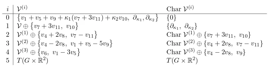
defined overG×R2. To apply the generalised Goursat normal form, Theorem 3, we work with
i V(i) CharV(i) 0 v1+v5+v9+κ1(v7+ 3v11) +κ2v10, ∂κ1, ∂κ2 {0}
1 V ⊕v7+ 3v11, v10 {∂κ1, ∂κ2}
2 V(1)⊕v4+ 2v8, v7−v11 CharV(1)⊕ {v7+ 3v11, v10} 3 V(2)⊕v4−2v8, v1+v5−5v9 CharV(2)⊕ {v4+ 2v8, v7−v11} 4 V(3)⊕v6, v1−3v5 CharV(3)⊕ {v4−2v8, v9}
5 T(G×R2) T(G×R2)
So hypotheses a), b) and c) of Theorem3are satisfied with q= 2 and derived lengthk= 5. Since q > 1, it remains to check the singular variety of the quotient V(4)/Char V(4). From the table we see that
CharV(4) =v4, v7, v8, v9, v10, v11, ∂κ1, ∂κ2
and
V(4)=v1, v4, v5, v6, v7, v8, v9, v10, v11, ∂κ1, ∂κ2
and hence
b
V(4):=V(4)CharV(4) =[v1], [v5], [v6] .
We obtain that Im ˆδ4 ={[v2], [v3]}and the polar matrix of the pointha1[v1] +a2[v5] +a3[v6]i ∈
PVb(4) is
−a2 a1 0 −a3 0 a1
which has unit rank if and only ifa1= 0. Hence the singular variety ofVb(4)isRP1 with singular bundle Bb=[v5],[v6] . Consequently, the resolvent bundle in this case is
RV(4)={v4, v5, v6, v7, v8, v9, v10, v11} ⊕ {∂κ1, ∂κ2}=sl(3,R)⊕R 2.
The resolvent bundle is integrable, showing that V(4) admits an integrable Weber structure, fulfilling hypothesis d) of Theorem 3. We can therefore conclude that Ωb⊥F is locally equivalent to the contact distributionC2(5) on jet space J5(R,R2).
For future reference, we note that we often abuse the term “derived type” by referring to the list of lists
dimV(j),dim CharV(j) kj=0
as the derived typeofV, wherekis its the derived length. Thus for the example just treated we may say that its derived type is
[3,0],[5,2],[7,4],[9,6],[11,8],[13,13]
since it is really the dimensions of these bundles that settles the recognitionproblem.
4.1 Dif ferential invariants via Contact
bundle, R(V(4)). The vector fields spanning this bundle are all vertical for the projection G×R3 → R3 and, indeed, they frame its fibres. It follows that the functions annihilated by
these vector fields are spanned byx,y,z– the coordinates of the homogeneous spaceG/SL(3,R)
in which the curves are immersed. Note that no integration is required6. A local coordinate calculation verifies this claim. By step b) we are at liberty to take any one of these as the parameter along the curve. We takex for this purpose. Continuing to follow b) we fix a vector field Z ∈ V such that Zx = 1. At this point we must construct the vector fields that span V. This is straightforward since V is constructed from the left-invariant vector fields onG (as well as∂κ1,∂κ2). We obtain
v1 =a1∂x+a4∂y+a7∂z, v2=a2∂x+a5∂y +a8∂z, v3 =a3∂x+a6∂y+a9∂z,
v4 =a1∂a1 −a3∂a3 +a4∂a4−a6∂a6+a7∂a7, v5=a2∂a1+a5∂a4 +a8∂a7, v6 =a3∂a1 +a6∂a4 +a9∂a7, v7 =a1∂a2+a4∂a5+a7∂a8,
v8 =a2∂a2 −a3∂a3 +a5∂a5−a6∂a6+a8∂a8, v9=a3∂a2+a6∂a5 +a9∂a8, v10=a1∂a3+a4∂a6, v11=a2∂a3 +a5∂a6, v12=∂κ1, v13=∂κ2,
where
a9= 1−a2a6a7+a1a6a8−a3a4a8+a3a5a7 a1a5−a4a2
.
From these we obtain
Z= 1 a1
v1+v5+v9+κ1(v7+ 3v11) +κ2v10
∈ V.
Note that Z is the total differential operator in this example. Finally, we let z1
0 = y, z02 = z as in step c) and compute the higher order coordinates as in step d) by differentiation by Z. This construction provides the components of the local equivalenceφ:G×R2→J5(R,R2) that
identifies V with the contact distribution C(5)2 onJ5(R,R2). Local inverse ψof the map φgives
the explicit differential invariants κ1,κ2, for curves inR3 up to “equi-affine motions”:
κ1=
24z22w3w5−35z22w42−60z2w23z4+ 60z2w3z3w4−24z2w2w3z5+ 70z2w4w2z4
−24z2w2z3w5+ 60w2w3z3z4−60w2z23w4−35w22z42+ 24z5w22z3(w3z2−w2z3)7/3,
κ2=
−18z23w3w4w5+ 25z23w34−36z22w33z5+ 90z22w23z4w4+ 36z22w32z3w5
−90z22w3z3w24+ 18z22w3w2z4w5+ 18z22w3w2w4z5−75z22w2w42z4+ 18z22w2z3w4w5 −90z2w23w2z24+ 72z2w32z5w2z3−18z2w3w22z4z5−72z2w3w2z32w5+ 90z2w2z32w24
+ 75z2w22w4z24−18z2w22z3w4z5−18z2w22z3z4w5+ 90w3w22z3z42−36w3z5w22z32
−25w32z43−90w22z32w4z4+ 18w32z3z4z5+ 36w22z33w5(w3z2−w2z3)7/2,
where zi =f(i)(x),wj =g(j)(x) for arbitrary smooth functionsf(x),g(x) such that
g′′′(x)f′′(x)−g′′(x)f′′′(x)6= 0.
Thus, if the curve in question has parametrisation (x, f(x), g(x)) then the complete set of differential invariants is {κ1, κ2}. Pulling back the remaining nonzero elements of the Maurer– Cartan form onGbyψgive explicit expressions for invariant differential one-forms onJ5(R,R2).
One can easily obtain the invariants in an arbitrary parametrisation of the curve or in terms of arclength parametrisation from these formulas but we won’t record these here7.
6See Section5for further comment on this aspect.
7Note that the inversion ofφis greatly assisted by the fact that the algebraic equations involved are guaranteed,
5
Curves in Riemannian manifolds
The geometries discussed in previous sections of this paper and the one treated in [28] are all of Klein type and one may wonder how the method fares when curvature is introduced. Also, in our previous (illustrative) examples, we have permitted ourselves knowledge of the explicit transitive group action in order to construct the differential system V and we do not want to make this assumption in general. In this paper we will be content to establish a result for Riemannian geometry and illustrate this by two examples. However, we conjecture that similar results hold for other Cartan geometries.
Letωi, πji be the components of the Cartan connection8 of an arbitrary Riemannian mani-fold (M, g), where dimM = n and ωi, 1 ≤ i ≤ n are semi-basic 1-forms for the projection F(M)→ M; F(M) is the orthonormal frame bundle over M. The structure equations for the coframe onF(M) are
We now state the main result of this section.
Theorem 4. Let n≥3andγ :I →M be an immersed curve in ann-dimensional Riemannian manifold (M, g), I ⊆ R. Let ωi, πi
j be the components of the Cartan connection for (M, g) on
the orthonormal frame bundle F(M)→M. Then
1. There is a unique integral submanifold of
V =
which projects to the Frenet lift of γ to the orthonormal frame bundle F(M).
2. The sub-bundle V is a uniform Goursat bundle with signature
h
n−1
z }| {
0,0, . . . ,0, n−1i.
Hence there is a local diffeomorphismφwhich identifies it with the contact distributionCn(n−1)
on jet space Jn(R,Rn−1).
3. The local diffeomorphism φ can be constructed by differentiation and algebraic operations alone.
4. If the isometries of (M, g) act transitively, then the local diffeomorphism φ induces lo-cal coordinate formulas for the complete invariants κ1
0, κ20, . . . , κn0−1 of the curve γ up to
isometries of (M, g).
Proof . The proofs of 1 and 4 are similar to the proof of Theorem1. The proof of 2 is complicated to write down in all generality; it is more enlightening to prove it in a sufficiently non-trivial case. We therefore write out the detail proof in the casen= 6, after which the general case will be clear.
The distribution in question, forn= 6, is
V =
We are required to prove that V ≃ C5(6). Let us arrange some of the frame elements into subsets as follows
determine a flag of Lie subalgebras. Using this we compute that for eachsin the range 1≤s≤6, the quotientsVbs:=V(s)/V(s−1) have basis representatives
Structure equations (12) show that the singular sub-bundle is
b
and therefore the resolvent bundle is given by
where a, b, i, j range over all possible values. These calculations show that that the derived type of V is
[[6,0],[11,5],[16,10],[21,15],[26,20],[31,25],[36,36]]
from which one deduce’s that the signature of V is h0,0,0,0,0,5i. Since R(V(5)) is integrable and all other hypotheses of Theorem3are satisfied withq= 5 andk= 6, we have shown thatV is locally equivalent to the contact systemC5(6) on J6(R,R5).
To prove 3, we invoke Theorem 4.2 of [28] which shows that to construct the local equiva-lence φ identifying V with C5(6) one only requires a complete set of invariants of the resolvent bundle R(V(5)). However, it is elementary to see that no element of R(V(5)) has components tangent toM; on the other handR(V(5)) spans the tangent spaces of the fibres overM. Hence, any coordinate system on M provides the needed invariants and no integration need be
per-formed.
In case the Riemannian manifoldM does not have a transitive isometry group thenV may simply be regarded as a control system on M with controls κ1n−2, κ2n−3, . . . , κn0−1 and with all other coordinates on E playing the role of state variables (outputs, in the language of control theory). The arc-length parametrisation along the curve plays the role of time in this control theoretic interpretation. The fact thatV is a Goursat bundle then proves that it isdifferentially flat, a type of control system currently under investigation in the control community. In fact it is currently a significant open problem in control theory to geometrically characterise all differentially flat control systems. One other way to state Theorem4is to say that the “natural” framing of curves in any Riemannian manifold is differentially flat.
IfM does possess a transitive isometry groupGthen the functionsκ10, . . . , κn0−1 form a com-plete set of curve invariants up to the action of G.
One may wonder whether Theorem4 is a genuine advance in the theory and/or practice of moving frames either in the sense of Cartan or in the sense of Fels–Olver. The contention of this paper is that it does represent an advance in both the theory and the practice of moving frames. As to the theory, I argue that endowing curves in a Cartan geometry with an explicit contact structure is significant given the fundamental role that contact structures play in ge-ometry and differential equations. As to the practice of the method of moving frames, in the case of Riemannian manifolds (M, g) we have given a framing for curves in M as solutions of a differential system ΩbF for any metric g and shown that it can be explicitly identified with
the contact system on a jet spaceJk(R,Rq) for somek,q. In case the isometry group of (M, g)
acts transitively, this identification delivers the complete set of invariant data including the differential curve invariants. We formulate this construction as an algorithm.
Algorithm Riemannian curves
INPUT: Riemannian manifold, (M, g), dimension n≥3.
a) Construct a parametrisation of SO(n) and orthonormal coframe ω on M.
b) Lift ω to the orthonormal frame bundle over M and build the Cartan connection Θ for (M, g). This involves linear algebra.
c) From Θ, build the differential system V defined in Theorem4.
d) Apply procedure Contact using, as invariants of the resolvent bundle, any coordinate system onM.
OUTPUT: Local diffeomorphismφidentifyingV with contact distributionCn(n−1) . In case the isometry group of (M, g) acts transitively, obtain complete, explicit invariant data for curves inM, following the inversion of φ.
Note that Riemannian curves is an algorithm in as much as steps a)–e) do not require any integration to be performed. All the steps involved are algebraic.
5.1 Curves in the Poincar´e half-space
The aim of this subsection is to apply the previous theorem to construct explicit expressions for curvature and torsion for curves in the Poincar´e half-space H3, with Riemannian metric
g= dx
2+dy2+dz2
z2 .
In principle we could approach this by putting coordinates on the Lie group SO(3,1) and then consider curves in the homogeneous space SO(3,1)/SO(3), as we did in the case of equi-affine space curves. However, this leads to unwieldy expressions which are difficult to handle, even with the help of a computer. Instead, we will use the method of equivalence to construct the Cartan connection for g and then use this to build the canonical Pfaffian system ΩF for the
Frenet frame of a generic curve inH3. In fact, we will construct the dual vector field distribution V = Ω⊥F.
to the orthonormal frame bundle F(H3) overH3 by
parametrisesSO(3). The fibres of the orthonormal frame bundleF(H3)→H3are diffeomorphic toSO(3) whose Maurer–Cartan form is theso(3)-valued 1-form
Ω =
and ωij+ωji = 0. As is usual in the method of equivalence, we compute the structure equations of the semi-basic forms obtaining
dω2 =ω21∧ω1+ω32∧ω3−(coscsinb+ sinacosbsinc)ω1∧ω2+ cosacosb ω2∧ω3, dω3 =ω31∧ω1+ω23∧ω2−(sinbcosc+ sinacosbsinc)ω1∧ω3
−(sinbsinc−sinacosbcosc)ω2∧ω3.
All torsion can be absorbed by redefining connection forms
π21 =ω21+ (sincsinb−sinacosbcosc)ω1−(sinacosbsinc+ sinbcosc)ω2, π31 =ω31+ cosacosbω1−(sinacosbsinc+ sinbcosc)ω3,
π32 =ω32+ cosacosbω2−(sinbsinc−sinacosbcosc)ω3,
and we obtain structure equations
dω1 =π12∧ω2+π31∧ω3, dω2=−π12∧ω1+π23∧ω3, dω3 =−π13∧ω1−π23∧ω2.
The remaining structure equations are
dπ21=−π13∧π23+ω1∧ω2, dπ31=π21∧π32+ω1∧ω3, dπ23 =−π21∧π31+ω2∧ω3.
These structure equations are those of the Maurer–Cartan form on SO(3,1). Moreover, we are now able to define the e(3)-valued Cartan connection
b
Ω =
0 0 0 0
ω1 0 π21 π31 ω2 π2
1 0 π32 ω3 π13 π23 0
,
with curvature
dΩ +b Ωb∧Ω =b
0 0 0 0
0 0 ω1∧ω2 ω1∧ω3 0 ω2∧ω1 0 ω2∧ω3 0 ω3∧ω1 ω3∧ω2 0
for metricg.
Setting n= 3 in (13), and adopting the usual notation κ1
0 =κ, κ20 =τ, κ11 = κ1, we study the integral submanifolds of
V =∂ω1 +κ∂π1
2 +τ ∂π23 +κ1∂κ, ∂κ1, ∂τ .
It is easy to check that V has derived type
[[3,0],[5,2],[7,4],[9,9]].
It can be checked thatρ1 =ρ2= 0 and hence the signature ofV ish0,0,2i. This is the signature of contact systemC2(3). To complete the check thatV is diffeomorphic to C2(3), we compute the resolvent bundle and check its integrability.
We find that CharV(2)={∂π2
3, ∂κ, ∂κ1, ∂τ}, and
V(2)/CharV(2) =∂ω1, ∂π1 2
, ∂π1 3 ,
whose structure is
[∂ω1, ∂π1
Hence, the singular bundle is Bb={[∂π1
2],[∂π31]} and consequently the resolvent bundle is
R(V(2)) =∂π1
2, ∂π13, ∂π23, ∂κ, ∂κ1, ∂τ =so(3)⊕
R3,
which is clearly integrable. An easy calculation in local coordinates verifies that the invariants of R(V(2)) are indeed the coordinates x, y, z on the base of the orthonormal frame bundle F(H3)→H3.
According to the Theorem we take one ofx,y, z as the independent variable. If y is taken for this purpose, then we can take D = ∂ω1 +κ∂π1
2 +τ ∂π32 +κ1∂κ as the direction of the total differential operator since 0 6= D (y) = −zcosasinc = µ. Then the operator of total differentiation is
Z=µ−1 ∂
ω1 +κ∂π1
2 +τ ∂π23 +κ1∂κ
.
Settingu=x, v=z, the remaining contact coordinates forVare then provided by differentiation
u1=Zu, v1 =Zv, u2=Zu1, v2 =Zv1, u3=Zu2, v3 =Zv2.
The mapφ
(x, y, z, a, b, c, κ, κ1, τ)7→(y, u, v, u1, v1, u2, v2, u3, v3)
pushes V forward toC2(3), which, in contact coordinates has the form
∂y+u1∂u+v1∂v+u2∂u1+v2∂v1+u3∂u2 +v3∂v2, ∂u3, ∂v3 .
A local inverse ofφis easily constructed and provides all the invariant data for curves inH3. In particular we deduce explicit expressions for curvature and torsion for curvesγ(y)=(u(y), y, v(y)), where for instanceu1,v2, denote derivativesdu/dy,d2v/dy2, etc. We obtain
κ=−u61+ 2u41v12+ 2u41vv2+ 3u41−2u31vu2v1+v14u21+ 2v12u21vv2+ 4u21vv2+u21v2v22
+ 4v12u21+ 3u21−2u1v2u2v1v2−2u1vu2v13−2u1v1u2v+ 1 +v41+v2u22v12+ 2v12vv2
+ 2vv2+v22v2+v2u22+ 2v12
1/2.
v12+u22+ 13/2,
τ =3u22u1+ 3u2v1v2+vu2v3−u3u21−u3v12−u3vv2−u3
v2.u22v2v21+u22v2
−2u2v2v1u1v2−2u2vv1u1−2v13u1u2v−2u31v1u2v+u21v2v22+v2v22+ 4u21vv2 + 2v21vv2+ 2vv2+ 2u41vv2+ 2v21u21vv2+ 1 + 2v21+v14+ 4u21v12+ 3u21+ 2u41v21
+v14u21+ 3u41+u61.
Once again, the algebraic system that is presented for solution in this task is guaranteed to have a block triangular structure.
We remark that semi-circular arcs parallel to they−z plane
γ(y) =C1, y,
q
C2 2 −y2
, C2>0, −C2 < y < C2
5.2 Curves in constant curvature Riemannian 3-manifolds
Let λ be any nonzero real number. Here we point out that the construction of the previous subsection can be carried out for the three dimensional Riemannian manifold (M(λ), gλ) with
metric
gλ =
dx2+dy2+dz2
1 + 4λ(x2+y2+z2)2
of constant curvature λ, where M(λ) is an open subset of R3. Exactly the same calculation as
before but with
for the metricgλ. Exactly the same calculation as the one carried out for the Poincar´e half-space
gives rise to the curvature and torsion for curves in (M(λ), gλ). We get
κλ=λ
The point to note here as in the previous example is that we are not required to know the explicit formulas for the action of the isometries on M(λ) before the invariants and the moving frame can be computed. Only infinitesimal data is required, in the form of the Cartan connection and then no integration need be performed.
Remark 4. Interestingly, τλ is not a continuous function ofλatλ= 0, while lim
λ→0κλ is not the curvature of the curve in the corresponding limiting metric lim
λ→0 gλ, which is Euclidean.
6
Closing remarks
We have also been concerned with the problem of explicitly computing differential invariants of curves immersed in spaces equipped with a transitive action of a Lie group. If this Lie group action is explicitly known and not too complicated then the method of choice for computing the differential invariants and other geometric data is the normalisation of the group action as in the equivariant moving frames method of Fels and Olver, described in [9,10]. This method is very general, has a simple and elegant theoretical foundation and presents as simple a computational task as could be hoped for. However, if the explicit group action is not known or it is known but too complicated to work with and if the goal is explicit expressions for differential invariants then the Fels–Olver method can’t readily be used to compute invariants explicitly9. In this case, we have shown that for Riemannian manifolds (M, g), the contact geometry can be fruitfully used to derive differential invariants and this requires as input data only the metricgand a rea-lisation of the structure group SO(n). With this data the Cartan connection for (M, g) can be constructed by linear algebra and differentiation. Subsequently, Theorem 4 provides an algo-rithm, Riemannian curves, for the curve invariants and, if required the Fels–Olver equivariant moving frame.
The symbolic computational aspects of procedureContactand algorithmRiemannian curves
presented in this paper should be mentioned briefly. TheMaplepackageDifferentialGeometry is ideally suited to the computation of all the relevant bundles and determining the derived type of any sub-bundle V ⊂ T M over manifold M. For instance, the two Riemannian examples presented in Section 5, take only a few minutes to complete commencing only with the met-ric and realisation of matrix group SO(3). Furthermore, the construction of differential curve invariants requires the inverse of the local diffeomorphism φ produced by procedure Contact. The proof of correctness of Contact in [28] shows that this algebraic problem will be block triangular. Thus the procedures discussed in this paper have quite good computational fea-tures.
However, of much greater significance stands the proposition that the Frenet frames along a curve and hence the curve itself can be endowed with a contact geometry. This shouldhave significance not only for the geometry of curves but also for Cartan’s method of moving frames as well as for the equivariant moving frames method of Fels and Olver. This is because contact systems are fundamental geometric objects and play a central role in differential geometry and differential equations. In fact, the construction of any contact system out of the components of a Cartan connection can in many ways replaceor complement the step by step construction of moving frames championed by Cartan. What is more, a characterisation of contact systems in arbitrary jet spaces in the spirit of the Goursat normal form is known [2, 30] and could be applied to study the geometry of submanifolds of dimension p >1 in general geometries as we have done here in the case p = 1. This raises the interesting question of the extent to which the results of this paper can be extended to homogeneous spaces in general and how they are connected to existing theory such as [5,6,8,12,14,11,26,1,21,9,10,24].
In this respect it should be mentioned that the Fels–Olver theory of moving frames has appli-cation well beyond the explicit calculation of differential invariants and moving frames. Much can be accomplished within the theory even without this explicit knowledge; see Mansfield [16] for details. What we hope to have achieved in this paper is the presention of evidence sup-porting the proposition that it is useful to enrich the philosophy and practice of moving frames by exploring its links with contact geometry.
Finally, we mention that an intriguing question is the relationship between the contact geo-metry of curves as explained here and the integrable motion of curves in various ambient mani-folds [13,7,17,19].
9However, it is sometimes possible to simplify the task of normalising the group action by using the known
Acknowledgements
I am indebted to the anonymous referees for insightful comments and for corrections which greatly improved the paper. Any remaining errors are mine.
References
[1] Alekseev D.V., Vinogradov A.M., Lychagin V.V., Geometry I,Encycl. Math. Sci., Vol. 28, Spinger-Verlag, Berlin, 1991.
[2] Bryant R.L., Some aspects of the local and global theory of Pfaffian systems, PhD thesis, University of North Carolina, Chapel-Hill, 1979.
[3] Bryant R.L., Chern S.S., Gardner R.B., Goldschmidt H.L., Griffiths P.A., Exterior differential systems, Mathematical Sciences Research Institute Publications, Vol. 18, Springer-Verlag, New York, 1991.
[4] Cartan ´E., La m´ethode du rep`ere mobile, la th´eorie des groupes continus et les espaces g´en´eralis´es Hermann & Cie, Paris, 1935.
[5] Cartan ´E., La th´eorie des groupes finis et continus et la g´eom´etrie diff´erentielle traitees par la m´ethode du rep`ere mobile, Gautier-Villars, Paris, 1937.
[6] Chern S.S., Moving frames, in The Mathematical Heritage of ´Elie Cartan (Lyon, 1984),Ast´erique, Vol. 1985, Numero Hors Serie, 1985, 67–77.
[7] Chou K.-S., Qu C.-Z., Integrable equations arising from motions of plane curves,Phys. D162(2002), 9–33. [8] Favard J., Cours de g´eom´etrie diff´erentielle locale, Gauthier-Villars, Paris, 1957.
[9] Fels M., Olver P.J., Moving coframes. I. A practical algorithm,Acta Appl. Math.51(1998), 161–213. [10] Fels M., Olver P.J., Moving coframes. II. Regularization and theoretical foundations, Acta Appl. Math.55
(1999), 127–208.
[11] Green M.L., The moving frame, differential invariants and rigidity theorems for curves in homogeneous spaces,Duke Math. J.45(1978), 735–779.
[12] Griffiths P.A., On Cartan’s method of Lie groups and moving frames as applied to uniqueness and existence questions in differential geometry,Duke Math. J.41(1974), 775–814.
[13] Ivey T., Integrable geometric evolution equations for curves, in The Geometrical Study of Differential Equations (Washington, DC, 2000), Contemp. Math., Vol. 285, Amer. Math. Soc., Providence, RI, 2001, 71–84.
[14] Jensen G.R., Higher order contact of submanifolds of homogeneous spaces,Lecture Notes in Mathematics, Vol. 610, Springer-Verlag, Berlin – New York, 1977.
[15] Kogan I.A., Inductive approach to moving frames and applications in classical invariant theory, PhD Thesis, University of Minesota, 2000.
[16] Mansfield E.L., A guide to the symbolic invariant calculus, Cambridge University Press, Cambridge, to appear.
[17] Mansfield E.L., van der Kamp P.E., Evolution of curve invariants and lifting integrability,J. Geom. Phys. 56(2006), 1294–1325.
[18] Olver P.J., Moving frames – in geometry, algebra, computer vision and numerical analysis, in Foundations of Computational Mathematics (Oxford, 1999), Editors R. DeVore, A. Iserles and E. S¨uli, London Math. Soc. Lecture Note Ser., Vol. 284, Cambridge University Press, Cambridge, 2001, 267–297.
[19] Olver P.J., Invariant submanifold flows,J. Phys. A: Math. Theor.41(2008), 344017, 22 pages.
[20] Shadwick W.F., Sluis W.M., Dynamic feedback for the classical geometries, in Differential Geometry and Mathematical Physics (Vancouver, BC, 1993), Contemp. Math., Vol. 170, Amer. Math. Soc., Providence, RI, 1994, 207–213.
[21] Sharpe R., Differential geometry. Cartan’s generalisation of Klein’s erlangen program, Graduate Texts in Mathematics, Springer-Verlag, New York, 1997.
[22] Spivak M., A comprehensive introduction to differential geometry, Vol. 1, Publish or Perish Press, 1970.
[23] Spivak M., A comprehensive introduction to differential geometry, Vol. 2, Publish or Perish Press, 1979.
[25] Stormark O., Lie’s structural approach to PDE systems,Encyclopedia of Mathematics and its Applications, Vol. 80, Cambridge University Press, Cambridge, 2000.
[26] Sulanke R., On ´E. Cartan’s method of moving frames,Colloq. Math. Soc. Janos Bolyai, Vol. 31, Differential Geometry, Budapest, 1979.
[27] Vassiliou P., A constructive generalised Goursat normal form,Differential Geom. Appl.24(2006), 332–350, math.DG/0404377.
[28] Vassiliou P., Efficient construction of contact coordinates for partial prolongations,Found. Comput. Math. 6(2006), 269–308,math.DG/0406234.
[29] Vessiot E., Sur l’int´egration des faisceaux de transformations infinit´esimales dans le cas o`u, le degr´e du faisceau ´etantn, celui du faisceau deriv´ee estn+ 1,Ann. Sci. ´Ecole Norm. Sup. (3)45(1928), 189–253. [30] Yamaguchi K., Contact geometry of higher order,Japan. J. Math. (N.S.)8(1982), 109–176.