Concordia University, Montr´eal, Quebec, Canada
Received January 05, 2007, in final form April 28, 2007; Published online May 15, 2007 Original article is available athttp://www.emis.de/journals/SIGMA/2007/066/
Abstract. We propose the graph description of Teichm¨uller theory of surfaces with marked points on boundary components (bordered surfaces). Introducing new parameters, we formu-late this theory in terms of hyperbolic geometry. We can then describe both classical and quantum theories having the proper number of Thurston variables (foliation-shear coordi-nates), mapping-class group invariance (both classical and quantum), Poisson and quantum algebra of geodesic functions, and classical and quantum braid-group relations. These new algebras can be defined on the double of the corresponding graph related (in a novel way) to a double of the Riemann surface (which is a Riemann surface with holes, not a smooth Riemann surface). We enlarge the mapping class group allowing transformations relating different Teichm¨uller spaces of bordered surfaces of the same genus, same number of boun-dary components, and same total number of marked points but with arbitrary distributions of marked points among the boundary components. We describe the classical and quantum algebras and braid group relations for particular sets of geodesic functions corresponding to An andDn algebras and discuss briefly the relation to the Thurston theory.
Key words: graph description of Teichm¨uller spaces; hyperbolic geometry; algebra of geo-desic functions
2000 Mathematics Subject Classification: 37D40; 53C22
1
Introduction
Recent advances in the quantitative description of the Teichm¨uller spaces of hyperbolic structures were mainly based on the graph (combinatorial) description of the corresponding spaces [19,7]. The corresponding structures not only provided a convenient coordinatization together with the mapping class group action, they proved to be especially useful when describing sets of geodesic functions and the related Poisson and quantum structures [3]. Combined with Thurston’s theory of measured foliations [22, 20], it led eventually to the formulation of the quantum Thurston theory [5]. The whole consideration was concerning Riemann surfaces with holes. A natural generalization of this pattern consists in adding marked points on the boundary components. First, Kaufmann and Penner [15] showed that the related Thurston theory of measured foli-ations provides a nice combinatorial description of open/closed string diagrammatic. Second, if approaching these systems from the algebraic viewpoint, one can associate a cluster algebra (originated in [10] and applied to bordered surfaces in [11]) to such a geometrical pattern.
The aim of this paper is to provide a shear-coordinate description of Teichm¨uller spaces of bordered Riemann surfaces, to construct the corresponding geodesic functions (cluster variables),
⋆This paper is a contribution to the Vadim Kuznetsov Memorial Issue ‘Integrable Systems and Related Topics’.
and to investigate the Poisson and quantum relations satisfied by these functions in classical case or by the correspondent Hermitian operators in the quantum case.
In Section2, we give a (presumably new) description of the Teichm¨uller space of bordered (or windowed) surfaces in the hyperbolic geometry pattern using the graph technique supporting it by considering a simplest example of annulus with one marked point. It turns out that adding each new window (a new marked point) increases the number of parameters by two resulting in adding a new inversion relation to the set of the Fuchsian group generators. We explicitly formulate rules by which we can construct geodesic functions (corresponding to components of a multicurve) using these coordinates; the only restriction we impose and keep throughout the paper is the evenness condition: an even number of multicurve lines must terminate at each window.
In Section 3, we construct algebras of geodesic functions postulating the Poisson relations on the level of the (old and new) shear coordinates of the Teichm¨uller space. We construct flip morphisms and the corresponding mapping class group transformations and find that in the bordered surfaces case we can enlarge this group allowing transformations that permute marked points on one of the boundary components or transfer marked points from one compo-nent to another thus establishing isomorphisms between all the Teichm¨uller spaces of surfaces of the same genus, same number of boundary components, and the same total number of marked points. In the same section, we describe geodesic algebras corresponding (in the cluster termi-nology, see [11]) to An and Dn systems. Whereas the An-algebras have been known previously as algebras of geodesics on Riemann surfaces of higher genus [16,17] (their graph description in the case of higher-genus surfaces with one or two holes see in [4]) or as the algebra of Stockes parameters [6, 23], or as the algebra of upper-triangular matrices [2], the Dn-algebras seem to be of a new sort. Using the new type of the mapping class group transformations, we prove the braid group relations for all these algebras.
Section4 is devoted to quantization. We begin with a brief accounting of the quantization procedure from [3] coming then to the quantum geodesic operators and to the corresponding quantum algebras. Here, again, the quantum Dn-algebras seem to be of a new sort, and we prove the Jacobi identities for them in the abstract setting without appealing to geometry. We also construct the quantum braid group action in this section.
In Section5, we describe multicurves and related foliations for bordered surfaces, that is, we construct elements of Thurston’s theory. There we also explicitly construct the relevant doubled Riemann surface, which, contrary to what one could expect, is itself a Riemann surface with holes (but without windows). We transfer the notion of multicurves to this doubled surface. Note, however, that the new mapping class group transformations, while preserving the mul-ticurve structure on the original bordered surface, change the topological type of the doubled Riemann surface, which can therefore be treated only as an auxiliary, not basic, element of the construction. Using this double, we can nevertheless formulate the basic statement similar to that in [5], that is, that in order to obtain a self-consistent theory that is continuous at Thurston’s boundary, we must set into the correspondence to a multicurve the sum of lengths of its constituting geodesics (the sum of proper length operators in the quantum case). In the same Section 5, we describe elements of Thurston’s theory of measured foliations for bordered Rie-mann surfaces and the foliation-shear coordinate changings under the “old” and “new” mapping class group transformations.
We discuss some perspectives of the proposed theory in the concluding section.
vertex, and is a maximum graph in the sense that after cutting along all its edges, the Riemann surface decomposes into the set of polygons (faces) such that each polygon contains exactly one hole (and becomes simply connected after plumbing this hole). Since a graph must have at least one face, we can therefore describe only Riemann surfaces with at least one hole, s > 0. The hyperbolicity condition also implies 2g−2 +s >0. We do not impose restrictions, for instance, we allow edges to start and terminate at the same vertex, allow two vertices to be connected with more than one edge, etc. We however demand a spine to be a cell complex, that is, we do not allow loops without vertices.
Then, we can establish a 1-1 correspondence between elements of the Fuchsian group and closed paths in the spine starting and terminating at the same directed edge. Since the terms in the matrix product depend on the turns in vertices (see below), it is not enough to fix just a starting vertex. To construct an element of the Fuchsian group ∆g,s, we select a directed edge (one and the same for all the elements; see the example in Fig.4where it is indicated by a short fat arrow), then move along edges and turns of the graph without backtracking and eventually turn back to the selected directed edge1.
We associate with theαth edge of the graph the realZα and set [7] the matrix of the M¨obius transformation
XZα =
0 −eZα/2
e−Zα/2 0
(2.1)
each time the path homeomorphic to a geodesic γ passes through the αth edge.
We also introduce the “right” and “left” turn matrices to be set in the proper place when a path makes the corresponding turn,
R=
1 1
−1 0
, L=R2=
0 1
−1 −1
,
and define the related operatorsRZ and LZ,
RZ≡RXZ=
e−Z/2 −eZ/2
0 eZ/2
,
LZ ≡LXZ =
e−Z/2 0
−e−Z/2 eZ/2
.
An element of a Fuchsian group has then the structure
Pγ=LXZnRXZn−1· · ·RXZ2RXZ1,
1If the last edge was not the selected one but its neighboring edge, the very last move is turning to the selected
edge, that is, we add eitherR- orL-matrix; if the last edge coincides with the selected edge, we do not make the last turn through the angle 2π. This results in the ambiguity by multiplication by the matrix−Id =R3, but it
and the correspondinggeodesic function
Gγ ≡ trPγ= 2 cosh(ℓγ/2) (2.2)
is related to the actual length ℓγ of the closed geodesic on the Riemann surface.
2.1.2 Generalization to the bordered surfaces case
We now introduce a new object, the markingpertaining to boundary components. Namely, we assume that we have not just boundary components but allow some of them to carry a finite number (possibly zero) of marked points. We letδi,i= 1, . . . , s, denote the corresponding num-ber of marked points for the ith boundary component. Geometrically, we assume these points to lie on the absolute, that is, instead of associating a closed geodesic to the boundary compo-nent in nonmarked case, we associate to anith boundary component a collection comprisingδi infinite geodesic curves connecting neighbor (in the sense of the surface orientation) marked points on the absolute (can be the same point if δi = 1) in the case where δi > 0. All these additional geodesic curves are disjoint with each other and disjoint with any closed geodesic on the Riemann surface. In [15], these curves were calledwindows. We denote the corresponding windowed surface Σg,δ, where
δ ={δ1, . . . , δs} (2.3)
is the multiindex counting marked points on the boundary components (δi can be zero) whereas
s is the number of boundary components. We call such Riemann surfaces the windowed, or bordered Riemann surfaces.
Restrictions ong,s, and the number of marked points #δ can be uniformly written ass >0 and 2g−2 +s+h#δ2+1i>0, that is, we allow two new cases g= 0, s= 1, #δ≥3 and g= 0,
s= 2, #δ≥1.
We want now to generalize the graph setting to the case where we have boundary components with marked points. However, as the example below shows, in order to define inambiguously the corresponding hyperbolic geometry, when introducing a marked point on the boundary, we must simultaneously introduce one more additional parameter. This is because, as we shall demon-strate, introducing a marked point adds a new inversion relation that preserves the orientation but not the surface itself, that is, we invert a part of the Riemann surface through a boundary curve without taking care on what happen to the (remaining) part of the surface because, in our description, this (outer) part is irrelevant. Such an inversion relation leaves invariant the new added geodesic, that is, the window. However, there is aone-parameter familyof such inversions for every window, and in order to fix the ambiguity we must indicate explicitly which point on the new geodesic is stable w.r.t. such an inversion. Recall that because of orientation preser-vation, two ends (on the absolute) of this new geodesic must be interchanged by the inversion relation; it is therefore a unique point that is stable.
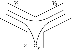
We describe this situation by consideringnew types of graphswith pending vertices. Assume that we have a part of graph having the structure as in Fig.1.
Then, if a geodesic line comes to a pending vertex, it undergoes theinversion, which stems to that we insert the inversion matrixF,
F =
0 1
−1 0
, (2.4)
into the corresponding string of 2×2-matrices. For example, a part of geodesic function in Fig.1 that is inverted reads
pending edge. Two types of geodesic lines are shown in the figure: one that does not come to the edge
Z is parameterized in the standard way, the other undergoes the inversion with the matrixF (2.4).
whereas the other geodesic that does not go to the pending vertex reads merely
· · ·XY1RXY2· · · .
We call this new relation the inversion relation, and the inversion element is itself an element of
P SL(2,R). We also call the edge terminating at a pending vertex thepending edge.
Note the simple relation2,
XZF XZ =X2Z.
We therefore preserve the notion of the geodesic function for curves with inversions as well. We consider all possible paths in the spine (graph) that are closed and may experience an arbitrary number of inversions at pending vertices of the graph. As above, we associate with such paths the geodesic functions (here, we letZi denote the variables of pending edges and Yj all other variables)
Gγ ≡ trPγ= 2 cosh(ℓγ/2) = trLXZnF XZnRXYn−1· · ·RXZ1F XZ1. (2.5)
We have that, for the windowed surface Σg,δ, the number of the shear coordinatesZα is
#Zα= 6g−6 + 3s+ 2 s
X
j=1
δj,
and adding a new window increases this number by two.
Before describing the general structure of algebras of geodesic functions, let us clarify the geometric origin of our construction in the simplest possible example.
2.2 Annulus with one marked point
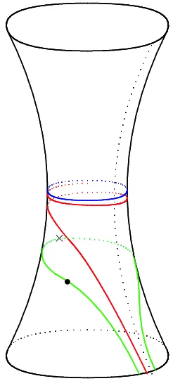
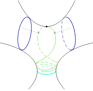
The simplest example is the annulus with one marked point on one of the boundary components (another example of disc with three marked points will be considered later). Here, the geometry is as in Fig. 2 where we let the closed line around the neck (the blue line) denote a unique closed geodesic corresponding to the element PI of the Fuchsian group to be defined below, the
winding to it line (the red line) is the boundary geodesics from the (ideal) triangle description due to Penner and Fock, and the lower geodesic (the green line) is the new line of inversion (the window). We indicate by bullet the stable point and by cross the point of the inversion line that is closest to the closed geodesic.
2In particular, we would consider inversion generated by a M¨obius element type, (2.1), say,F =X
W not just
Figure 2. Geodesic lines on the hyperboloid: dotted vertical line is the asymptote going to the marked point on the absolute, closed blue line is a unique closed geodesic; red line is the line from the ideal triangular decomposition asymptotically approaching the asymptote by one end and the closed geodesic by the other; green line is the line of inversion whose both ends approach the marked point; we let the bullet on this line denote the unique stable point under the inversion and the cross denote the point that is closest to the closed geodesic.
The same picture in the Poincar´e upper half-plane is presented in Fig.3. There, the whole domain in Fig. 2 bounded below by the bordered (green) geodesic line and above by the neck geodesic (blue) line is obtained from a single ideal triangle with the vertices{eZ+Y,∞,0} upon gluing together two (red) sides of this ideal triangle. We now construct two (hyperbolic) ele-ments: PI that is the generating element for the original hyperbolic geometry and the new
element PII that corresponds to the inversion w.r.t. the lower (green) geodesic line in Figs. 2
and 3. Adding this new element obviously changes the pattern, but because the Fuchsian pro-perty retains, the quotient of the Poincar´e upper half-plane under the action of this new Fuchsian group must be again a Riemann surface with holes. As we demonstrate below, this new Riemann surface is just the double of the initial bordered Riemann surface.
For this, we use the graph representation. The corresponding fat graph is depicted in Fig.4. This graph with one pending edge and another edge that starts and terminates at the same vertex is dual to an ideal triangle{eZ+Y,∞,0}in which two (red) sides are glued one to another (the resulting curve is dual to the loop) and the remaining (green) side is the boundary curve (dual to the pending edge). We mark the starting direction by the fat arrow, so the elementPIis
PI=XZLXYLXZ =
e−Y /2+eY /2 −eZ+Y /2
e−Z−Y /2 0
. (2.6)
Apparently, the corresponding geodesic function GI is just e−Y /2 +eY /2, so the length of the
closed geodesic is |Y|as expected.
We now construct the element PII. Note that this element makes the inversion w.r.t. the
Figure 3. The hyperbolic picture corresponding to the pattern in Fig.2: preimages of red boundary line are red half-circles, preimages of the inversion line are green half circles (the selected one connects the points∞and 0 on the absolute), and the preimage of the closed geodesic is the (unique) blue half-circle; the pointseZandeZ+Y on the absolute are stable under the action of the corresponding Fuchsian element PI (2.6); the bullet symbols are preimages of the point that is stable upon inversion (the one that lies
on the geodesic line between∞and 0 isi in the standard coordinates on the upper half-plane) and the dotted half-circles connect the point eZ+Y with its images (one of which is −e−Z−Y) under the action of the inversion elementF. We also mark by cross the pointieZ+Y /2
of the green geodesic line that is closest to the closed geodesic. The invariant axis of the new element PII (2.7) and some of its images
under the action of (2.6) are depicted as cyan half-circles;ξ2 is from (2.8).
to left, this matrix will be rightmost). Then, the rest is just the above element PI:
PII=XZLXYLXZF =PIF =
eZ+Y /2 0
e−Y /2+eY /2 e−Z−Y /2
, (2.7)
and the corresponding geodesic functionGIIis 2 cosh(Z+Y /2) so the length of the corresponding
geodesic (but in a geometry still to be defined!) is|2Z+Y|.
We now consider the action of these two elements in the geometry of the Poincar´e upper half-plane in Fig. 3. It is easy to see that the element PI has two stable points: eZ (attractive) and
eZ+Y (repulsive). It also maps ∞ →0, eZ+eZ+Y → ∞, etc. thus producing the infinite set of preimages of the red geodesic line in Fig.2 upon identification under the action of this element. The element F first interchanges 0 and ∞ and eZ+Y and −e−Z−Y thus establishing the inversion (inversion) w.r.t. the green geodesic line. The only stable point of this inversion is the point of intersection of the two above geodesic lines, and it is the pointi in the upper complex half-plane for every Z +Y. Further action is given by PI and, in particular, it maps ∞ back
to 0, so ξ1= 0 is a stable point of PII. Another stable point is
ξ2 =
eZ+Y /2−e−Z−Y /2
eY /2+e−Y /2 , (2.8)
and it is easy to see that the two invariant axes of PI and PII never intersect. Adding the
element PII to the set of generators of the new extended Fuchsian group we therefore obtain
a new geometry.
Figure 4. The graph for annulus with one marked point on one of the boundary components. Examples of closed geodesics without inversion (I) and with inversion (II) are presented. The short fat arrow indicates the starting direction for elements of the Fuchsian group.
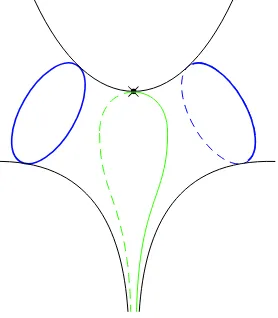
Figure 5. The doubled Riemann surface obtained upon inversion w.r.t. the green geodesic in the case where the stable point coincides with the point closest to the closed geodesics (blue line) (the cross then coincides with the bullet).
we chop out all its part that is below the green (inversion) line. We then obtain the doubleof the Riemann surface merely by inverting it w.r.t. the green line taking into account the obvious (mirror) symmetry that takes place in this case. We then obtain from the hyperboloid with marked point at the boundary component the sphere with two identical cycles (images of the closed geodesic) and one additional puncture (hole of zero length), as shown in Fig. 5.
What happens if, instead of the stable point marked by cross, we have arbitrary stable point (bullet in Figs. 2 and 3)? Actually, we can answer this question just from the geometrical standpoint. Indeed, since in the pattern in Fig. 2, points on the inversion geodesics that lie to both sides from the asymptote are close, they must remain close in the new geometry. But the image of each such point is shifted by a distance that is twice the distance D (along the inversion line, which is a geodesic line) between the stable point (bullet) and the symmetric point (cross). This means that, in the new geometry, the points on the inversion line separated by a distance 2D must be asymptotically close as approaching the absolute in the pattern of Fig.3. This means in turn that the corresponding geodesic in the new geometry is just a geodesic approaching the new closed geodesic of length 2D.
It remains just to note that, from the pattern in Fig.3,
Figure 6. The doubled Riemann surface obtained upon inversion w.r.t. the green geodesic in the case where the stable point (marked by•) is arbitrary. The closed in the asymptotic geodesic sense points in the new geometry are those on different coils of the spiraling green geodesics, which has the asymptotic form of the double helix. The separation length is asymptotically equal to|2Z+Y|. The cyan line is the new closed geodesic (the invariant axis of the element PII). We let two crosses denote the points on the
inversion line that are closest to the two copies of the initial closed geodesic line; the geodesic distance between them is also|2Z+Y|.
that is, the perimeter of the new hole is |2Z +Y|, and it coincides with the length of the new element PII (2.7), which is therefore the element of the new, extended, Fuchsian group
corresponding to going round the new hole. In Fig. 6, we depict this new geometry. It is also interesting to note that we now again, as in the symmetrical case, have two (homeomorphic) images of the initial bordered surface, but the union of these two images in Fig. 6 constitutes only the part of the corresponding Riemann surface that is above the new closed geodesics (the cyan line); two ends of the green geodesics constitute the double helix approaching the new geodesic line but never reaching it, and we always have one copy of the initial surface on one side of coils of this helix and the other copy – on the other side.
3
Algebras of geodesic functions
3.1 Poisson structure
One of the most attractive properties of the graph description is a very simple Poisson algebra on the space of parameters Zα. Namely, we have the following theorem. It was formulated for surfaces without marked points in [7] and here we extend it to arbitrary graphs with pending vertices.
Theorem 1. In the coordinates(Zα) on any fixed spine corresponding to a surface with marked
points on its boundary components, the Weil–Petersson bracket BWP is given by
BWP=
X
v
3
X
i=1
∂ ∂Zvi
∧ ∂
∂Zvi+1
, (3.1)
where the sum is taken over all three-valent(i.e., not pending)verticesvandvi,i= 1,2,3 mod 3,
are the labels of the cyclically ordered edges incident on this vertex irrespectively on whether they are internal or pending edges of the graph.
Proposition 1. The center of the Poisson algebra (3.1)) is generated by elements of the form
P
Zα, where the sum is over all edges of Γ in a boundary component ofF(Γ) taken with
multi-plicities. This means, in particular, that each pending edge contributes twice to such sums. Proof . The proof is purely technical; for the case of surfaces without marked points on bound-ary components it can be found in Appendix B in [5]. When adding marked points, it is straightforward to verify that the sums in the assertion of the proposition are central elements. In order to prove that no extra central elements appear due to the addition process, it suffices to verify that the two changes of the part of a graph shown below,
do not change the corank of the Poisson relation matrix B(Γg,s,δ).
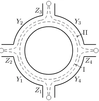
Example 1. Let us consider the graph in Fig. 8. It has two boundary components and two
corresponding geodesic lines. Their lengths, P4 i=1
Yi and
4
P
i=1
(Yi+ 2Zi), are the two Casimirs of the
Poisson algebra with the defining relations
{Yi, Yi−1}= 1 mod 4, {Zi, Yi}=−{Zi, Yi−1}= 1 mod 4,
and with all other brackets equal to zero.
3.2 Classical f lip morphisms and invariants
The Zα-coordinates (which are the logarithms of cross ratios) are called(Thurston) shear
coor-dinates [22,1] in the case of punctured Riemann surface (without boundary components). We preserve this notation and this term also in the case of windowed surfaces.
In the case of surfaces with holes, Zα were the coordinates on the Teichm¨uller space Tg,sH, which was the 2s-fold covering of the standard Teichm¨uller space ramified over surfaces with punctures (when a hole perimeter becomes zero, see [8]). We assume correspondinglyZα to be the coordinates of the corresponding spaces Tg,δH in the bordered surfaces case.
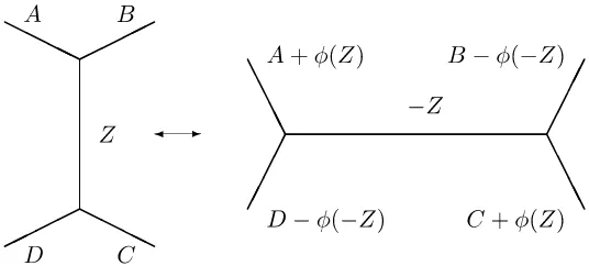
Assume that there is an enumeration of the edges of Γ and that edgeαhas distinct endpoints. Given a spine Γ of Σ, we may produce another spine Γαof Σ by contracting and expanding edgeα of Γ, the edge labelled Z in Fig.7, to produce Γα as in the figure; the fattening and embedding of Γα in Σ is determined from that of Γ in the natural way. Furthermore, an enumeration of the edges of Γ induces an enumeration of the edges of Γα in the natural way, where the vertical edge labelledZ in Fig.7corresponds to the horizontal edge labelled −Z. We say that Γα arises from Γ by aWhitehead movealong edgeα. We also write Γαβ = (Γα)β, for any two indicesα,β of edges, to denote the result of first performing a move alongαand then alongβ; in particular, Γαα = Γ for any indexα.
3.2.1 Whitehead moves on inner edges
Proposition 2 ([3]). Setting φ(Z) = log(eZ+ 1)and adopting the notation of Fig. 7 for shear coordinates of nearby edges, the effect of a Whitehead move is as follows:
WZ : (A, B, C, D, Z)→(A+φ(Z), B−φ(−Z), C+φ(Z), D−φ(−Z),−Z). (3.2)
Figure 7. Flip, or Whitehead move on the shear coordinatesZα. The outer edges can be pending, but the inner edge with respect to which the morphism is performed cannot be a pending edge.
B′ = B−2φ(−Z); if A = B (or C = D), then A′ = A+Z (or C′ = C+Z); if A = D (or
B =C), then A′ =A+Z (or B′ =B+Z). Any variety of edges amongA, B, C, and D can
be pending edges of the graph.
We also have two simple but important lemmas establishing the properties of invariance w.r.t. the flip morphisms.
Lemma 1. Transformation (3.2) preserves the traces of products over paths (2.5).
Lemma 2. Transformation (3.2) preserves Poisson structure (3.1) on the shear coordinates.
That the Poisson algebra for the bordered surfaces case is invariant under the flip transfor-mations follows immediately because we flip here inner, not pending, edges of a graph, which reduces the situation to the “old” statement for surfaces without windows.
We also have the statement concerning the polynomiality of geodesic functions.
Proposition 3. All Gγ constructed by (2.5) are Laurent polynomials in eZi and eYj/2 with
positive integer coefficients, that is, we have the Laurent property, which holds, e.g., in cluster algebras [10]. All these geodesic functions preserve their polynomial structures upon Whitehead moves on inner edges, and all of them are hyperbolic elements (Gγ > 2), the only exception
where Gγ = 2 are paths homeomorphic to going around holes of zero length (punctures).
3.2.2 Whitehead moves on pending edges
In the case of windowed surfaces, we encounter a new phenomenon as compared with the case of surfaces with holes. We can construct morphisms relatinganyof the Teichm¨uller spacesTH
g,δ1
and TH
g,δ2 with δ1 = {δ11, . . . , δn11} and δ2 = {δ12, . . . , δn22} providing n1 = n2 = n and n1
P
i=1
δ1
i = n2
P
i=1
δ2i, that is, we explicitly construct morphisms relating any two of algebras corresponding
to windowed surfaces of the same genus, same number of boundary components, and with the same total number of windows; the window distribution into the boundary components can be however arbitrary.
This new morphism corresponds in a sense to flipping a pending edge.
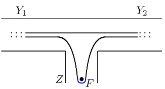
Lemma 3. Transformation in Fig. 9is the morphism between the spaces TH
g,δ1 andTg,δH2. These morphisms preserve both Poisson structures (3.1) and the geodesic length functions. In Fig. 9
Figure 8. An example of geodesics whose geodesic functions are in the center of the Poisson algebra (dashed lines). WhereasGI corresponds to the standard geodesic around the hole (no marked points are
present on the corresponding boundary component), the line that is parallel to a boundary component with marked points must experience all possible inversions on its way around the boundary component, as is the case forGII.
Figure 9. Flip, or Whitehead move on the shear coordinates when flipping the pending edgeZ(indicated by bullet). Any (or both) of edgesY1and Y2 can be pending.
Proof . Verifying the preservation of Poisson relations (3.1) is simple, whereas for traces over paths we have four different cases of path positions in the subgraph in the left side of Fig. 9, and in each case we have the corresponding path in the right side of this figure3. In each of these cases we have the followingmatrixequalities (each can be verified directly)
XY2LXZF XZLXY1 =XY˜2LXY˜1,
XY1RXZF XZRXY1 =XY˜1LXZ˜F XZ˜RXY˜1,
XY2RXY1 =XY˜2RXZ˜F XZ˜RXY˜1,
XY2LXZF XZRXY2 =XY˜2RXZ˜F XZ˜LXY˜2,
where (in the exponentiated form)
eY˜1 =eY1 1 +e−2Z−1, eY˜2 =eY1 1 +e2Z, eZ˜ =e−Z.
From the technical standpoint, all these equalities follow from flip transformation (3.2) upon the substitution A = C = Y2, B = D = Y1, and Z = 2Z. The above four cases of geodesic
3We can think about the flip in Fig.9as about “rolling the bowl” (the dot-vertex) from one side to the other;
around the dot-vertex, we set the inversion matrixF.
functions are then exactly four possible cases of geodesic arrangement in the (omitted) proof of Lemma 1.
Using flip morphisms in Fig.9 and in formula (3.2), we may establish a morphism between any two algebras corresponding to surfaces of the same genus, same number of boundary compo-nents, and same total number of marked points on these components; their distribution into the boundary components can be however arbitrary. And it is again a standard tool that if, after a series of morphisms, we come to a graph of the same combinatorial type as the initial one (dis-regarding marking of edges), we associate a mapping class groupoperation with this morphism therefore passing from the groupoid of morphisms to the group of modular transformations.
Example 2. The flip morphism w.r.t. the edgeZ1 in the pattern in (3.3),
(3.3)
where Z1 and Z2 are the pending edges, generates the (unitary) mapping class group
transfor-mation
eZ2 →e−Z1, eZ1 →eZ2 1 +e−2Z1−1, eY →eY 1 +e2Z1
on the corresponding Teichm¨uller space Tg,δH. This is a particular case of braid transformation to be considered in detail in Section 3.6.
3.3 New graphical representation
In the case of usual geodesic functions, there exists a very convenient representation in which one can apply classical skein and Poisson relations in classical case or the quantum skein relation in the quantum case and ensure the Riedemeister moves when “disentangling” the products of geodesic function representing them as linear combinations of multicurve functions. However, in our case, it is still obscure what happens when geodesic lines intersect in some way at the pending vertex. In fact, we can propose the comprehensive graphical representation in this case as well! For this, let us come back to Fig. 1 and resolve now the inversion introducing a new
dot-vertex at a pending vertex inside the fat graph and assuming that the inversion matrix F
corresponds to winding around this dot-vertex as shown in Fig.10.
3.3.1 Classical skein relation
The trace relation tr (AB) + tr (AB−1)− trA· trB = 0 for arbitrary 2×2 matrices Aand B
with unit determinant allows one to “disentangle” any product of geodesic functions, i.e., express it uniquely as a finite linear combination of generalized multicurves (see Definition 2 below). Introducing the additional factor #Gto be the total number of components in a multicurve, we can uniformly present the classical skein relation as
(3.4)
We assume in (3.4) that the ends of lines are joint pairwise in the rest of the graph, which is the same for all three items in the formula. Of course, we perform there algebraic operations with the algebraic quantities – with the (products of) geodesic functions corresponding to the respective families of curves.
3.3.2 Poisson brackets for geodesic functions
We first mention that two geodesic functions Poisson commute if the underlying geodesics are disjointly embedded in the sense of the new graph technique involving dot-vertices. Because of the Leibnitz rule for the Poisson bracket, it suffices to consider only “simple” intersections of pairs of geodesics with respective geodesic functions G1 and G2 of the form
G1 = tr1· · ·XC1R1XZ1L1XA1· · · , (3.5)
G2 = tr2· · ·XB2L2XZ2R2XD2 · · ·, (3.6)
where the superscripts 1 and 2 pertain to operators and traces in two different matrix spaces. The positions of edgesA, B, C, D,andZare as in Fig.7. Dots in (3.5), (3.6) refer to arbitrary sequences of matricesR1,2,L1,2,X1,2
Zi, andF
1,2belonging to the corresponding matrix spaces;G 1
andG2 must correspond to closed geodesic lines, but we make no assumption on their simplicity
or graph simplicity, that is, the paths that correspond toG1 and G2 may have self- and mutual
intersections and, in particular, may pass arbitrarily many times through the edge Z in Fig. 7. Direct calculations then give
{G1, G2}= 1
2(GH−GI), (3.7)
whereGIcorresponds to the geodesic that is obtained by erasing the edgeZ and joining together
the edges “A” and “D” as well as “B” and “C” in a natural way as illustrated in the middle diagram in (3.4);GH corresponds to the geodesic that passes over the edgeZ twice, so it has the
form tr · · ·XCRZRD· · · ·XBLZLA· · · as illustrated in the rightmost diagram in (3.4). These relations were first obtained in [12] in the continuous parametrization (the classical Turaev–Viro algebra).
Having two curves, γ1 and γ2, with an arbitrary number of crossings, we now find their
Poisson bracket using the following rules:
Figure 11. An example of two geodesic lines intersecting at the dot-vertex. We present four homotopical types of resolving two intersections in this pattern (Cases (a)–(d)). Case (d) contains the loop with only the dot-vertex inside. This loop is trF = 0, so the whole contribution vanishes in this case. The (green) factors in brackets pertain to the quantum case in Section 4 indicating the weights with which the corresponding (quantum) geodesic multicurves enter the expression for the productG~
1G ~ 2.
• If, in the course of calculation, we meet an empty (contractible) loop, then we associate the factor−2 to such a loop; this assignment, as is known [5], ensures the Riedemeister moves on the set of geodesic lines thus making the bracket to depend only on the homotopical class of the curve embedding in the surface.
• If, in the course of calculation, we meet a curve homeomorphic to passing around a dot-vertex, then we set trF = 0 into the correspondence to such curve thus killing the whole corresponding multicurve function.
These simple and explicit rules are an effective tool for calculating the Poisson brackets in many important cases below.
Because the Poisson relations are completely determined by homotopy types of curves in-volved, using Lemma 3, we immediately come to the following theorem
Theorem 2. Poisson algebras of geodesic functions for the bordered Riemann surfaces Σg,δ1 and Σg,δ2 that differ only by distributions of marked points among their boundary components are isomorphic; the isomorphism is described by Lemma 3.
Figure 12. Generating graphs forAn algebras forn= 3,4, . . .. We indicate character geodesics whose geodesic functionsGij enter bases of the corresponding algebras.
3.4 The An algebras
Consider the disc with n marked points on the boundary; examples of the corresponding rep-resenting graph Γn are depicted in Fig. 12 for n = 3,4, . . .. We enumerate the n dot-vertices clockwise,i, j= 1, . . . , n. We then letGij withi < j denote the geodesic function corresponding to the geodesic line that encircles exactly two dot-vertices with the indices i and j. Examples are in the figure: forn= 3, red line corresponds toG12, blue – toG23 and green – toG13. Note
that in the cluster terminology (see [11]) these algebras were called theAn−2-algebras.
Using the skein relation, we can close the Poisson algebra thus obtaining forA3:
{G12, G23}=G12G23−2G13 and cycl. permut. (3.8)
Note that the left-hand side is doubled in this case as compared to Nelson–Regge algebras recalled in [5]. In theA3, case this is easily understandable because, say,
G12= trLX2Z2RX2Z1 =e
Z1+Z2 +eZ1−Z2+e−Z1−Z2, (3.9)
and this expression literally coincides with the one for the algebra of geodesics in the case of higher genus surfaces with one or two holes (see [4]) but the left-hand side of the relation is now doubled (the analogous expression forG12 in [4] was the same as in (3.9) upon the substitution
Z1 = X1/2 and Z2 = X2/2, but with the X-variables having the doubled Poisson brackets {X2, X1}= 2). In higher-order algebras (starting withn= 4), we meet a more complicate case
of the fourth-order crossing (as shown in the casen= 4 in Fig.12). Using our rules for Poisson brackets, we find that those for these geodesic functions are
{G13, G24}= 2G12G34−2G14G23 (3.10)
(note that the items in the products in the r.h.s. mutually commute).
It is also worth mentioning that after this doubling that occurs in the right-hand sides of relations (3.8) and (3.10), we come exactly to algebras appearing in the Frobenius manifold approach [6].
3.5 The Dn-algebras
We now consider the case of annulus with nmarked points on one of the boundary component (see the example in Fig. 8. Here, again, the state of art is to find a convenient (finite) set of geodesic functions closed w.r.t. the Poisson brackets4. In the case of annulus, such a set is given by geodesic functions corresponding to geodesics in Fig. 13.
We therefore describe a set of geodesic functions by the matrixGij withi, j= 1, . . . , nwhere the order of indices indicates the direction of encompassing the second boundary component of the annulus.
Figure 13. Typical geodesics corresponding to the geodesic functions constituting a set of generators of the Dn algebra. We let Gij, i, j = 1, . . . , n, denote these functions. The order of subscripts is now important: it indicates the direction of encompassing the hole (the second boundary component of the annulus). The most involved pattern of intersection is on the right part of the figure: the geodesics have there eight-fold intersection; in the left part we present also the geodesic functionGii corresponding to the geodesic that starts and terminates at the same window.
Lemma 4. The set of geodesic functions Gij corresponding to geodesics in Fig. 13 is Poisson
closed.
The relevant Poisson brackets are too cumbersome and we omit them here because one can easily read them from the corresponding quantum algebra in formula (4.13) below in the limit as~→0.
3.6 Braid group relations for windowed surfaces
3.6.1 Braid group relations on the level of Z-variables
We have already demonstrated in Example 2a m.c.g. relation interchanging two pending edges of a graph. In a more general case of An-algebra, we have a graph depicted in Fig. 12 and another intertwining relation arises from the three-step flipping process schematically depicted in Fig. 14.
The graph for the An algebra has the form in Fig. 12 with Yi, 2 ≤ i ≤ n−2, being the variables of internal edges and Zj, 1≤j≤n, being the variables of the pending edges and we identify Y1 ≡Z1 and Yn−1≡Zn to make formulas below uniform.
We letRi,i+1 denote the intertwining transformation in Fig.14for 2≤i≤n−2 and in Fig.9
fori= 1 and i=n−1. For the exponentiated variables, these transformations have the form
Figure 14. Three-step flip transformation of intertwining pending edge variables Zi and Zi+1 that
results in the same combinatorial graph. The rest of the graph denoted by dots remains unchanged.
Rn−1,n
The following lemma is the direct calculation using (3.11), (3.12), and (3.13).
Lemma 5. For any n≥3, we have the braid group relation
Ri−1,iRi,i+1Ri,i−1=Ri,i+1Ri−1,iRi,i+1, 2≤i≤n−1.
3.6.2 Braid group relations for geodesic functions of An-algebras
Here we, following Bondal [2], propose another, simpler way to derive the braid group relations using the construction of the groupoid of upper-triangular matrices. It was probably first used in [6] to prove the braid group relations in the case ofA3 algebra. In the case ofAn algebras for general n, let us construct the upper-triangular matrix A
A=
associating the entries Gi,j with the geodesic functions. Using the skein relation, we can then present the action of the braid group elementRi,i+1exclusively in terms of the geodesic functions
from this, fixed, set:
A very convenient way to present this transformation is by introducing the special matrices
Bi,i+1 of the block-diagonal form
ij
this chain of transformations, G(i,ii−+11) =G1(0),i+1 =G1,i+1, and the whole chain of matricesB can
be then expressed in terms of the initial variables Gi,j as
B ≡Bn−1,nBn−2,n−1· · ·B2,3B1,2 =
and the whole action onA gives
˜
and we see that it boils down to a mere permutation of the elements of the initial matrixA. It is easy to see that the nth power of this permutation gives the identical transformation, so we obtain the lastbraid group relation.
Lemma 6. For any n≥3, we have the second braid group relation
Rn−1,nRn−2,n−1· · ·R2,3R1,2n= Id.
3.6.3 Braid group relations for geodesic functions of Dn-algebras
It is possible to express readily the action of the braid group on the level of the geodesic functions
Gi,j,i, j= 1, . . . , n, interpreted also as entries of the n×n-matrix D(the elements that are not
The first braid group relation follows in this case as well from the three-step process, but it can be verified explicitly that the following lemma holds.
Lemma 7. For any n≥3, we have the braid group relationfor transformations (3.16):
Ri−1,iRi,i+1Ri,i−1D=Ri,i+1Ri−1,iRi,i+1D, 2≤i≤n−1.
Note that the second braid-group relation (see Lemma6) is lost in the case of Dn-algebras. To present the braid-group action in the matrix-action (covariant) form (3.15) note that the combinations Gk,j, Gj,k, and Gk,kGj,j have similar transformation laws in (3.16) in the case where at least one of the indicesjandkis neitherinori+ 1, so we can try to construct globally covariantly transformed matrices from linear combinations of the above (coefficients of these combinations can be different above and below the diagonal). Note that (since the braid-group transformation acts on theAnsubgroup ofDnin the same way as before), the matricesA(3.14) and AT are transformed as in (3.15); the analysis shows that we also have two new matrices, R and S, with the sametransformation law as in (3.15):
(R)i,j =
Gj,i+Gi,j−Gi,iGj,j j > i, −Gj,i−Gi,j+Gi,iGj,j j < i,
0 j=i,
(3.17)
(S)i,j =Gi,iGj,j for all 1≤i, j≤n, (3.18)
where Ris skewsymmetric (RT =−R) and S is symmetric (ST =S).
Lemma 8. Any linear combination w1A+w2AT +ρR+σS with complex w1, w2, ρ, and σ transforms in accordance with formula (3.15) under the braid-group action.
We postpone the discussion of modular invariants constructed from these four matrices till the discussion of the quantum Dnbraid-group action in Section 4.5.2.
4
Quantum Teichm¨
uller spaces of windowed surfaces
4.1 Canonical quantization of the Poisson algebra
A quantization of a Poisson manifold, which is equivariant under the action of a discrete groupD, is a family of ∗-algebras A~
depending on a positive real parameter ~ with D acting by outer
automorphisms and having the following properties:
1. (Flatness.) All algebras are isomorphic (noncanonically) as linear spaces.
2. (Correspondence.) For~= 0, the algebra is isomorphic as aD-module to the ∗-algebra of
complex-valued functions on the Poisson manifold.
3. (Classical Limit.) The Poisson bracket onA0 given by{a
1, a2}= lim ~→0
[a1,a2]
~ coincides with
the Poisson bracket given by the Poisson structure of the manifold.
Fix a cubic fatgraph Γg,δ as a spine of Σg,δ, and let T~=T~(Γg,δ) be the algebra generated by Z~
α, one generator for each unoriented edgeα of Γg,δ, with relations
[Zα~, Zβ~] = 2πi~{Zα, Zβ} (4.1)
(cf. (3.1)) and the∗-structure
structure is nondegenerate on the quotient T /Z .
The examples of suchboundary-parallel curves are again in Fig. 8. Of course, those are the same curves that provide the center of the Poisson algebra.
A standard Darboux-type theorem for nondegenerate Poisson structures then gives the fol-lowing result.
Corollary 1. There is a basis forT~
/Z~
given by operatorspi,qi, fori= 1, . . . ,3g−3+s+ s
P
j=1
δj
satisfying the standard commutation relations [pi, qj] = 2πi~δij.
Now, define the Hilbert space H to be the set of allL2 functions in theq-variables and let each q-variable act by multiplication and each corresponding p-variable act by differentiation,
pi = 2πi~∂q∂i. For different choices of diagonalization of non-degenerate Poisson structures, these Hilbert spaces are canonically isomorphic.
4.2 Quantum f lip transformations
The Whitehead move becomes now a morphism of (quantum) algebras. Thequantum Whitehead move orflipalong an edge of Γ by equation (3.2) is described by the (quantum) function [3]
φ(z)≡φ~(z) =−π~
2
Z
Ω
e−ipz
sinh(πp) sinh(π~p)dp, (4.2)
where the contour Ω goes along the real axis bypassing the origin from above. For each un-bounded self-adjoint operatorZ~
onH,φ~
(Z~
) is a well-defined unbounded self-adjoint operator on H.
The functionφ~
(Z) satisfies the relations (see [3])
φ~
(Z)−φ~
(−Z) =Z,
φ~(Z+iπ~)−φ~
(Z−iπ~) = 2πi~
1 +e−Z,
φ~(Z+iπ)−φ~(Z−iπ) = 2πi 1 +e−Z/~
and is meromorphic in the complex plane with the poles at the points{πi(m+n~), m, n∈Z+}
and {−πi(m+n~), m, n∈Z+}.
The functionφ~
(Z) is therefore holomorphic in the strip|ImZ|< πmin (1,Re~)−ǫfor any
ǫ >0, so we need only its asymptotic behavior as Z ∈Rand |Z| → ∞, for which we have (see,
e.g., [14])
φ~(Z)|Z|→∞= (Z+|Z|)/2 +O(1/|Z|).
Theorem 3. The family of algebras T~
= T~
(Γg,δ) is a quantization of Tg,δH for any cubic
fatgraph spine Γg,δ of Σg,δ, that is,
• In the limit ~ 7→ 0, morphism (3.2) using (4.2) coincides with classical morphism (3.2) with φ(Z) = log(1 +eZ).
• Morphism (3.2) using (4.2) is indeed a morphism of∗-algebras.
• A flip WZ satisfiesWZ2 =I, (3.2), and flips satisfy the commutativity relation. • Flips satisfy the pentagon relation.
• The morphisms T~
(Γ)→ T1/~
(Γ) given by Z~
α 7→Z
1/~
α commute with morphisms (3.2).
4.3 Geodesic length operators
We next embed the algebra of geodesic functions (2.2) into a suitable completion of the con-structed algebra T~
. For any γ, the geodesic function Gγ can be expressed in terms of shear coordinates on TH:
Gγ ≡ trPZ1···Zn =
however distinguish between them as soon as they come from different products of exponentials
e±Zi/2 in traces of matrix products in (4.3).
where the quantum ordering × ×·
×
× implies that we vary the classical expression (4.3) by
intro-ducing additional integer coefficients cj(γ, α), which must be determined from the conditions below.
That is, we assume that each term in the classical expression (4.3) can get multiplicative corrections only of the form qn,n∈Z, with
q ≡e−iπ~.
We often call a quantum geodesic function merely a quantum geodesic because quantum objects admit only a functional description.
We now formulate the defining properties of quantum geodesics.
1. If closed pathsγ and γ′ do not intersect, then the operatorsG~
γ and G
3. Geodesic algebra. The product of two quantum geodesics is a linear combination of quan-tum multicurves governed by the (quanquan-tum) skein relation below.
:ea1ea2· · ·ean: = 1 + (a
We have [3] the proposition, which can be extended to the case of windowed surfaces assuming the modification of the “old” notion of graph simple geodesics.
Definition 1. For a spine Γg,δ, we call a geodesicgraph simpleif it does not pass twice through any of inner edges of the graph and has at most one inversion at any of pending edges.
Proposition 4. For any graph simple geodesic γ with respect to any spine Γ, the coefficients
cj(γ, α) in (4.4) are identically zero, i.e., the quantum ordering is the Weyl ordering. Proof . Let us again denote byY~
i ,i= 1, . . . ,6g−6 + 3s+ #δ, the quantum shear coordinates of inner edges and by Z~
j, j= 1, . . . ,#δ the quantum shear coordinates of pending edges. But the latter always come in the combinationXZ~
jF XZ
~
j =X2Z
~
j, so, considering term-by-term the
trace of the matrix product for a quantum graph simple geodesic, we find that we can expand it in Laurent monomials in eYi~/2 andeZ
~
j. It is easy to see that each termeYi~/2 and eZ
~
j comes
either in power +1, or−1 in the corresponding monomial and there are no equivalent monomials in the sum. This means that in order to have a Hermitian operator, we must apply the Weyl ordering with no additional q-factors (by the correspondence principle, each such factor must be again a Laurent monomial in q standing by the corresponding term, which breaks the self-adjointness unless all such monomials are unity). Since quantum Whitehead moves must preserve the property of being Hermitian, if a graph-simple geodesic transforms to another graph-simple geodesic, then a Weyl-ordered expression transforms to a Weyl-ordered expression, and only
these expressions are self-adjoint.
Example 3. For theA3 algebra graph in Fig. 12, we have exactly three graph simple geodesics
with the corresponding geodesic functionsG~ 12,G
~
23, andG ~
13given by formulas (3.9) (which are
written already in the Weyl-ordered form), and if we consider, for instance, the product
G~23G~12=q−1G~1232+qG~13, (4.6)
where G~
1232 and G ~
13 correspond to respective cases (a) and (b) of resolving crossing of the
geodesics γ23 and γ12 near the dot-vertex 2 in Fig. 11. Note that G~13 is also Weyl-ordered,
G13=eZ3+Z1 +eZ3−Z1 +e−Z3−Z1 whereas
G~1232 =eZ1+2Z2+Z3 +eZ1+2Z2−Z3 +eZ1−2Z2−Z3 +e−Z1−2Z2−Z3+ (q2+q−2)eZ1−Z3
4.4 Quantum skein relations
We now formulate thegeneralrules that allow one to disentangle the product of any two quantum geodesics.
Let G~
1 and G ~
2 be two quantum geodesic operators corresponding to geodesics γ1 and γ2
where all the inversion relations are resolved using the dot-vertex construction (see Fig. 10). Then
• We must apply the quantum skein relation6
(4.7)
simultaneouslyatallintersection points.
• After the application of the quantum skein relation we can obtain empty (contractible) loops; we assign the factor −q −q−1 to each such loop and this suffices to ensure the quantum Riedemeister moves.
• We can also obtain loops that are homeomorphic to going around a dot-vertex; as in the classical case, we claim the corresponding geodesic functions to vanish, so we disregard all such cases of geodesic laminations in the quantum case as well.
The main lemma is in order.
Lemma 10 ([3, 21]). There exists a unique quantum ordering × ×· · ·
×
× (4.4), which is generated
by the quantum geodesic algebra (4.7)and is consistent with the quantum mapping class groupoid transformations (3.2), i.e., so that the quantum geodesic algebra is invariant under the action of the quantum mapping class groupoid.
4.5 Quantum braid group relation
4.5.1 Quantum An-algebra
We now consider the quantum geodesic functions associated with paths in theAn-algebra pattern in Fig. 12. From the quantum skein relation, it is easy to obtain quantum transformations for the quantum geodesic functionsG~
i,j. We introduce theA
associating the Hermitian operators G~
i,j with the quantum geodesic functions. Using the skein relation, we can then present the action of the braid group element R~
i,i+1 exclusively in terms
6Here the order of crossing lines corresponding to G~
1 andG
~
2 depends on which quantum geodesic occupies
form
Then, the action of the quantum braid group generator R~
i,i+1 on A ~
can be expressed as the matrix product (taking into account the noncommutativity of quantum matrix entries)
R~
the matrix Hermitian conjugate toB~
i,i+1 (its nontrivial 2×2-block has the form
qG~
i,i+1 1
q2 0
). Using the same technique as above, it is then straightforward to prove the
following lemma.
Lemma 11. For anyn≥3, we have the quantum braid group relations
R~i−1,iR~i,i+1R~i−1,i=R~i,i+1R~i−1,iR~i,i+1, 2≤i≤n−1, (4.11)
R~n−1,nRn~−2,n−1· · ·R~2,3R~1,2n= Id. (4.12)
4.5.2 Quantum Dn-algebra
We now quantize the Poisson algebra of geodesic functionsGij corresponding to paths as shown in Fig. 13. We have there eight possible variants of nontrivial intersections shown in Fig.15.
The corresponding quantum permutation relations read7 (q =e−iπ~
,ξ ≡q2−q−2)
7Deriving these relations requires a tedious combinatorial analysis based on quantum skein relations formulated
Figure 15. Eight cases of nontrivial intersections of geodesics from the set Gij, i, j = 1, . . . , n in the case of the Dn-algebra.
Case (c) [G~ik, G~jl] =ξ
G~jkG~il−G~jiG~lk
;
Case (d) qG~jlG~kj−q−1G~kjG~jl=ξG~kl; (4.13)
Case (e) [G~jl, G~lj] =ξ
(G~ll)2−(G~jj)2
;
Case (f) [G~
jl, G
~
ii] =ξ
G~
jiG
~
ll−G
~
ilG
~
jj
;
Case (g) qG~jjG~kj−q−1G~kjG~jj =ξG~kk, qG~jkG~jj−q−1G~jjG~jk =ξG~kk;
Case (h) [G~
ii, G
~
kk] = (q−q−1) G
~
ik−G
~
ki
.
Although these relations not only contain triple terms in the r.h.s. but also noncommuting terms (this is the price for closing the algebra), they nevertheless establish the lexicographic ordering on the corresponding set of quantum variables {G~
ij}.
Lemma 12. Permutation relations treated as an abstract algebra postulated by (4.13) satisfy the commutation Jacobi identities.
The proof is tedious but straightforward calculations. Note that algebra (4.13) is self-consistent even without relation to geometry of modular spaces; the similar phenomenon was already observed in the case of An-algebras. As regarding the classification of cluster algebras in [11], we produced the corresponding algebras for disc and annulus with arbitrary number of marked points (in our approach, a punctured disc is just an annulus with one hole of zero perimeter; using the isomorphism in Theorem2we can move all marked points to one boundary component). We do not know however as yet an example of such an algebraically closed set for a disc with two punctures (holes); this case deserves a separate investigation.
Lemma 13. For any n≥3, we have thequantum braid group relations (4.11) for transforma-tions (4.14) of quantum operators subject to quantum algebra (4.13).
Again, it the second identity (4.12) is lost in the case of Dn algebras.
4.5.3 Matrix representation for Dn-algebra and invariants
We now construct the quantum analogues of (3.17) and (3.18).
Lemma 14. The following four matrices (with operatorial entries), together with all their linear combinations, transform in accordance with the quantum braid-group action (4.10): A~
(4.8),
Remark 1. We took particular form8 (4.15) of the matrix R~
because, in the case n= 2, the combination
G~1,1G~2,2−qG~1,2−q−1G~2,1 =G~2,2G~1,1−q−1G~1,2−qG~2,1
is a central element of the (quantum) algebra D2; the other central element is
G~1,2G~2,1−q2(G~2,2)2−q−2(G~1,1)2 =G~2,1G~1,2−q−2(G2~,2)2−q2(G~1,1)2.
Also, exactly with such a combination, diagonal elements remain zeros acquiring noq-corrections. And, eventually, only this matrix possesses the (quantum) cyclic symmetry below.
A cyclic permutation of indicesP : i7→i+ 1 modn; j7→j+ 1 modndestroys the structure of the matrixA~
and results in the following transformations for R~
and S~
8Recall that we can “play” with coefficients adding matricesA~
and A~†
These transformations together with (4.10) generate a full modular group. This means that, at least in the classical case, detR is the mapping-class group invariant and lies therefore in the center of the Poisson algebra. Same is true for S, but detS ≡ 0 whereas detR is nonzero for even n = 2m (and vanishes for odd n): denoting Qi,j := (R)i,j for i < j, we have that detR= Pf (R)2, where the Pfaffian Pf (R) is given by the Grassmann-variable integral
Pf (R) =
Z
· · ·
Z
dθ1· · ·dθ2me
P
1≤i<j≤2m θiQi,jθj
and is described by all possible (signed) pairings in the setθ1θ2· · ·θ2m−1θ2m wherehθiθji=Qi,j fori < j.
For example, form= 2, we have
I4 =Q1,2Q3,4+Q1,4Q2,3−Q1,3Q2,4
(recall thatQi,j =Gi,j+Gj,i−Gi,iGj,j in the classical case). In the quantum case, these elements obviously getq-corrections to be calculated explicitly since the notion of a quantum determinant is ambiguous; we hope to return to this problem elsewhere.
Also, this construction provides just one central element of the algebra D2m; finding other central elements in a regular way (similar to the one in [2] where all the central elements of the
An-algebra were generated by det(λ−1A+λAT)) needs further investigation.
5
Multicurves and the double of windowed surface
5.1 Multicurves for bordered surfaces
It is a standard notation that a multicurve (lamination) is a collection of non(self)intersecting curves. Apparently, in a new formulation with dot-vertices, this definition can be literally transferred to the case of surfaces with marked points on boundary components.
Definition 2. Consider the homotopy class of a finite collection Ce={γ1, . . . , γn}of disjointly embedded (unoriented) simple curves γi in a topological windowed surface Σg,δ. These curves are either closed or terminate at windows. We impose the only restriction that we have an even (can be zero) number of endpoints of these curves at each window. An even-based generalized multicurve (eGMC) Ce in Σg,δ is a multiset based on C; we then have si ≥1 parallel copies of components ofC, or in other words, positive integral weightssi on each component ofC, where
si is the multiplicity ofγiinCe. Further, given a hyperbolic structure on Σg,δ, we associate toCe the product
GCe =G s1 γ1· · ·G
sn γn
of geodesic operators (2.2) of all geodesics constituting a GMC; these operators Poisson commute in the classical case since the components of C are disjoint.
We therefore extend the standard definition by introducingnonclosedcurves that terminate at the boundary components. The only restriction we impose is the evenness of the number of curves terminating at each connected part of a boundary component (passing through an inversion geodesic line). Now in order to obtain the multicurve, we connect pairwise the ends of these curves (below the inversion, or bounding, geodesic line) as shown in Fig. 16 obtaining therefore the collection of topologically closedcurves.
denote the dot-vertex. Lower (yellow) part is fictitious and is not present in the original geometry of surfaces with boundaries.
5.2 The double of the Riemann surface
In order for our procedure to have a geometrical sense, we now construct the double of the Riemann surface and transfer to this double the structure of multicurves. Note that it is often easier to prove properties of the geodesic function using the structure of the doubled Riemann surface without boundary components.
We first describe the doubled surface itself. Nonintersecting curves must remain noninter-secting in the picture of double when we replace inversions merely by (doubled) variables 2Zi on the corresponding edges. To attain this, let us consider the example of a geodesic line in Fig. 17. If we clone this surface, drift apart the copy of it and then connect all the pending ends with their twins preserving the orientation (as shown in Fig. 18), then we obtain the new Riemann surface without pending edges (and, correspondingly, without windows). Having the initial Riemann surface Σg,δ where δ is from (2.3), s the number of boundary components, and δj the number of marked points on thejth component (can be zero), we obtain that upon the joining as shown in Fig.18, each boundary component withevenδj (including the zero one) generates two boundary components without marked points (holes) in the doubled Riemann surface, whereas each boundary component with odd δj generates exactly one hole in the new doubled Riemann surface. Then, easy calculation using the Euler characteristic formula gives the answer for the genus ˆg and number of holes ˆsof the doubled Riemann surface Σˆg,ˆs:
ˆ
g= 2g−1 +1 2
s
X
j=1
δj+ #{oddδj}
, sˆ= 2s−#{odd δj}. (5.1)
Note that while flip morphisms on inner edges of the initial graph pertain to flipping simulta-neously two (disjoint) copies of this edge in the double graph, flip morphisms on pending edges (see Fig.9) change the topological structure of the double graph (the genus and the number of holes of the doubled Riemann surface may then change; only the total Poisson dimension must remain invariant).
As in the case of dual Teichm¨uller spaces in [8], the coordinatesZαdescribe the linear subspace of the Teichm¨uller spaceTH
ˆ
g,ˆs, which is again a 2sˆ-fold covering of the Teichm¨uller space ramified over punctured surfaces (with old and new boundary components). This subspace comprises surfaces admitting the involution interchanging two halves of the doubled Riemann surface.
Figure 17. An example of geodesic curve with even number of inversions.
experiences two inversions while curve II has one inversion. To produce a multicurve on the doubled surface, we first merely double the pattern (first stage in Fig. 19) and then connect each pending edge of the original graph with its copy on the clone of this graph in a natural way, that is, preserving the orientation and without introducing intersections of threads of the multicurve (second stage in Fig.19).
We note, first, that the pattern in the doubled surface thus obtained is always a multicurve (since we did not introduce any new intersection). We now turn to its content.
It is easy to see that a geodesic line I with the geodesic function GI and the length ℓI on
the original surface that hasevennumber of inversions producestwodisjoint nonselfintersecting (albeit not parallel) geodesic lines I1 and I2 on the doubled Riemann surface, and these two new
lines has the respective geodesic functions GI1 andGI2 and lengths ℓI1 and ℓI2 such that
GI1 =GI2 =GI, ℓI1 =ℓI2 =ℓI. (5.2)
On the contrary, for a geodesic line II with the geodesic function GII and the length ℓII
that has an odd number of inversions, this geodesics produces one nonselfintersecting geodesic line II1,2on the doubled Riemann surface with the geodesic functionGII1,2 and lengthℓII1,2, and
it is easy to see that they satisfy the relations
GII1,2 = (GII)
2−2, ℓ
II1,2 = 2ℓII, (5.3)
that is, we have then a single geodesic of doubled length.
From (5.2) and (5.3) it follows that we must take as the characteristic of a multicurve, or a rational lamination, the sum of lengths of the constituent geodesics. We must be able to construct this sum from the geodesic function or from a quantum geodesic function ensuring the positiveness property: the length must be nonnegative function in the classical case or positive-definite operator in the quantum case. This is ensured by the following construction proposed in [5].
Definition 3. The proper length p.l.(γ) ≡ ℓγ of a closed curve γ in the classical or quantum case is constructed from the quantum geodesic operator G~
γ as
p.l.(γ)≡ℓγ= 2 lim n→∞
1
nlog 2Tn(G
~
Figure 18. The double representation for the Riemann surface depicted in Fig.17. Pending propagators on boundary components are connected, each carrying the doubled shear coordinate 2Zi, in a crosswise manner. We then obtain an oriented surface whose genus is given by (5.1). To each nonselfintersecting geodesic line that has an even number of inversions in the original picture, we may set into the correspon-dence a unique (nonselfintersecting) line on the doubled Riemann surface (dashed line for the geodesic line in Fig.17).
where we take the principal branch of the logarithm and Tn are Chebyshev’s polynomials (cf. (4.5)). Since Tn(cosh2t) = coshnt2, it follows that p.l.(γ) is the hyperbolic length of γ in the Poincar´e metric in the classical case.
In the operatorial case, we can determine p.l.(γ) explicitly in terms of the spectral expansion of the operatorG~
γ, which is known exactly [14]. Namely, the basis of eigenfunctions ofG
~
γis labeled by the positive numberS whereas the eigenvalue corresponding to the eigenfunction|αSihas the form eS/2+e−S/2 and the both limitsS →+∞and S→0 are singular in the functional sense.
Eigenfunctions |αSi constitute an orthogonal and complete basis, so we can define the proper length operator to be the one with the same eigenfunctionsαS and with positive eigenvaluesS/2. The operator p.l.(γ) is then a well-defined operator on any compactum in the function spaceH. The proper length of a QMC or GMC ˆC, which we denote as p.l.( ˆC) ≡ ℓCˆ, is the sum of
the proper lengths of the constituent geodesic length operators (or the sum of geodesic lengths calculated in the Poincar´e metric in the classical case) weighted by the number of appearances in the multiset.
Lemma 15. Given a general even-based multicurveCe, its proper length
ℓCe ≡ n
X
i=1
siℓγi, (5.4)
satisfies the general relation: denoting by Cb1,2 the GMC generated on the doubled Riemann surface, we have
ℓCb
1,2 = 2ℓCe