www.elsevier.nl / locate / econbase
Life-cycle modeling of bequests and their impact on
annuity valuation
a,b ,* Alain Jousten a
´
CORE, Universite catholique de Louvain, 34 Voie du Roman Pays, B-1348 Louvain-la-Neuve,
Belgium
b
´
Universite libre de Bruxelles, Bruxelles, Belgium Received 30 August 1998; accepted 30 March 1999
Abstract
In this paper we introduce a linear bequest motive into a standard life-cycle model, both allowing for credit and annuity market imperfections. First, we characterize the consump-tion and wealth processes. We find that consumpconsump-tion is non-increasing in the linear bequest parameter for the simplest certainty case, but that the same is not true for life-span uncertainty. Second, we study the issue of annuity valuation. For a sufficiently strong bequest motive, the true value of an annuity is equal to the actuarial value. This invalidates a previous claim that, for imperfect annuity markets, it is close to the simple financial value.
2001 Elsevier Science B.V. All rights reserved.
Keywords: Bequests; Annuities; Consumption function; Elderly
JEL classification: D11; H55
1. Introduction
Bequest motives have long been recognized as potentially important deter-minants of saving patterns. Surprisingly, there has been very little work directed at describing how they affect optimal consumption patterns. We add a utility of
´
*CORE, Universite catholique de Louvain, 34 Voie du Roman Pays, B-1348 Louvain-la-Neuve, Belgium.
E-mail address: [email protected] (A. Jousten).
1
bequests term of the joy-of-giving type to a standard life-cycle model. We use a quasi-linear utility function in consumption and bequests and allow for both life-span uncertainty and liquidity constraints. We study the consumption and wealth profiles towards the end of the life-cycle. We focus on the behavior of people who have retired from active work and who are or will be eligible for some form of annuitized government benefits.
Within our framework we analyze two questions. First, we characterize the consumption and wealth profile of the elderly in the presence of a bequest motive. Even though joy-of-giving models have already been used before, a characteriza-tion of their impact on the consumpcharacteriza-tion and wealth profile, both in a setup with and without liquidity constraints, is missing. Second, we analyze the implications for the valuation of annuity contracts, such as, for example, retirement income schemes.
The liquidity constraints analyzed mimic the U.S. law, which prohibits the use of social security benefits as collateral. The importance of liquidity constraints is indicated inter alia by the results of Hausman and Paquette (1987). The authors found strong empirical evidence of jumps in consumption levels at the time involuntary early retirees become eligible for retirement benefits. The finding of consumption jumps at the time of first eligibility implies that the legal limitations actually matter, and that the market does not completely offset them through private arrangements.
We find that the presence of a bequest motive has strong implications for the valuation of annuity contracts. Previously, Bernheim (1987) claimed that, in the presence of liquidity constraints, the value of a marginal dollar of annuity payouts
2
is close to the simple financial value of future payouts. With sufficiently strong bequest motives, this does not apply: the true value of a marginal annuity payout stream is close to the actuarially correct value, which takes into account both the interest rate and the survival probabilities. Annuity valuation is of considerable importance for some of today’s most acute policy questions, particularly the evaluation of reforms in the area of old-age income provision. For example, to evaluate and understand the implications of a move from a public annuity based retirement income systems towards a private pension savings system, a good measure of the value of annuity holdings is crucial.
Our paper is divided into two main parts. First, we characterize the implications
1
This modelling strategy follows Yaari (1965), Fischer (1973), Friedman and Warshawsky (1988) and Hurd (1989).
2
of a bequest motive on consumption and wealth. In Section 2, we start by presenting a certainty model with potentially binding liquidity constraints. We find that consumption levels are non-increasing in the strength of the bequest motive. Section 3 extends the analysis to the case of a life-span uncertainty model, both with and without liquidity constraints. We find that the previous result does not generalize to this more realistic setup. That is, consumption at some ages can be higher for a person with a stronger bequest motive. Further, we establish that, under life-span uncertainty, the rate of growth of consumption is non-decreasing in the strength of the bequest parameter. Section 4 constitutes the second part of the paper, where we analyze the question of annuity valuation in the presence of a bequest motive. Section 5 contains some concluding remarks.
2. Certainty model
Consider an individual who lives for two periods (t5h0,1j). Suppose that we can represent his utility function by
B
1 2
]] ]]]
U(C ,C ,B )0 1 2 5u(C )0 111ru(C )1 1b 2, (1)
(11r)
where the first two terms correspond to the standard additively separable utility of consumption (C0 and C ) terms. We suppose that the per period utility of1
3
consumption function is strictly concave, and that limC→0u9(C )5 `. r denotes the real interest rate the individual faces on the capital markets and r is the discount rate for utility generated by consumption.
The third term in expression (1) captures the utility generated by bequests that we assume to be realized at the time of death and to be linear in the present discounted value of bequests B with the linear parameter2 b. There are several reasons for choosing this linear form. The first reason is tractability, as it would be more difficult to derive clear predictions in a general setup. Second, the quasi-linearity of the utility function of consumption and bequests captures the reasonable assertion that people are less risk averse with respect to bequests than with respect to their own personal consumption.
Further, notice that we use different discount factors for consumption (r) and bequests (r). Jousten (1998) shows that the choice of r as the discount rate for bequests is very convenient. First, a linear bequest motive with discount rate r is equivalent to a more general linear motive allowing for both a gift and a bequest
3
motive. Second, this particular setup allows us to abstract away from timing issues
4
with respect to these gifts and bequests.
The use of the interest rate r for discounting utility of bequests further allows us to reinterpret the utility-of-bequests term in the utility function. Instead of viewing it as a discounted period 2 utility, we can see the bequest terms as a linear function of the present discounted value of bequests, which is our preferred interpretation in this paper.
Suppose that the individual has an initial wealth W and is entitled to an income0
Y in period 1. Further suppose that the individual faces credit constraints. We can1
then write the consumer’s problem as the following constrained optimization problem:
1 b
]] ]]]
Max
S
u(C )0 111ru(C )1 1 2B2D
,C ,C ,B0 1 2 (11r)
s.t.
S;W02C0$0, (2)
Y1 C1 B2
]] ]] ]]]
W0111r5C0111r1 2, (3)
(11r)
B2$0, (4)
where the first constraint represents the credit constraint at the end of the first period and the second the global resource constraint. We further impose an explicit non-negativity constraint on bequests (expression (4)). The assumption of having marginal utility tend to infinity as consumption levels tend to zero takes care of the non-negativity of the two consumption variables C and C .0 1
2.1. Kuhn–Tucker problem
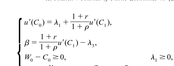
Using the Kuhn–Tucker method, we can find the following optimality con-ditions:
4
11r
]]
u9(C )0 5l 11 11ru9(C ),1
11r]]
b 511ru9(C )1 2l3,
W02C0$0, l $1 0, l1(W02C )0 50,
Y1 C1 B2]] ]] ]]]
W0111r5C0111r1 2,
(11r)
B $0, l $0, l B 50,
2 3 3 2wherel1 and l3 are the Kuhn–Tucker multipliers associated with the inequality constraints (2) and (4), respectively.
We can regroup the possible optima into four different scenarios depending on the binding or the slackness of the two inequality constraints. We split the analysis of the optimality conditions into two parts. First we derive equations for the borders delimiting these four scenarios depending on which constraints are binding. Then, in a second step, we characterize the four possible scenarios.
2.1.1. The borders
We derive the equations of the expressions delimiting the different scenarios in terms of the bequest parameterb and the period 1 income level Y keeping total1
lifetime income R;W01[Y /(11 1r)] constant. Noticing that when a constraint
switches from slackness to binding, both the constraint and the associated Kuhn– Tucker multiplier equal 0, we can derive equations for the expressions that delimit the border between the four scenarios. As we will see, the constraints will have the shape shown in Fig. 1.
The expression separating the binding and slackness of the credit constraint can be written as
* * Y15Y ,1 forb , b ,
(5)
H
b 5u9hR2[Y /(11 1r)]j, forb $ b*,*
where Y1 is the implicit solution to u9hR2[Y /(11 1r)]j5[(11r) /(11r)]u9(Y )1
* *
andb is the solution tob 5[(11r) /(11r)]u9(Y ). Notice that because of our1
*
assumption of unbounded marginal utility at a zero consumption level, Y1 is strictly positive.
Characterizing this function (5), it is easy to see that Y is non-decreasing in1 b
because of the sign of u99(.). Further, depending on the sign of the third derivative of the utility function, the expression is either concave or non-concave. For example, for the case of a CRRA utility function, the function is concave.
Similarly, the expression for the bequest constraint is
* *
b 5 b , for Y1#Y ,1
(6)
H
b 5[(11r) /(11r)]u9(Y ),1 for Y1.Y .*1This functional form implies that Y is decreasing in1 b and that the concavity depends on the sign of u999(.). For the case of a CRRA utility function, function (6) is non-convex.
Fig. 1 illustrates the borders and the four scenarios they delimit. Eq. (6) is represented by the dotted line, and Eq. (5) by the continuous line. The dashed vertical line at R(11r) represents total income expressed in period 1 units.
2.1.2. The four scenarios
2.1.2.1. Scenario 1: No constraint binding
We start by checking the benchmark case of having both the bequest and liquidity constraint not binding, i.e. l 51 0 and l 53 0. In this case, we have
u9(C )0 5[(11r) /(11r)]u9(C )1 5b. Hence, dC / d0 b ,0 and dC / d1 b ,0. Fur-ther, it is easy to see that dS / db .0 and that dB / d2 b .0.
2.1.2.2. Scenario 2: Credit constraint binding
The optimum is characterized by the following conditions: [(11r) /(11 r)]u9(C )1 5b and W05C . These two conditions imply that dC / d0 0 b 50 and dC / d1 b ,0, as well as dS / db 50 and dB / d2 b .0. A third relation that holds at the optimum shows us that the liquidity constraint also becomes less binding. Indeed, the above results combined with u9(C )0 5l 11 [(11r) /(11r)]u9(C )1
2.1.2.3. Scenario 3: Bequest constraint binding
A third possible scenario is when constraint (4) is the only binding constraint. We hence have l .3 0. In this case, the allocation of resources between consumption in the first and second period follows the standard equation u9(C )0 5
[(11r) /(11r)]u9(C ). Further, the budget constraint (3) simplifies to W1 01[Y /1
(11r)]5C01[C /(11 1r)]. It is thus trivial to find dC / d0 b 5dC / d1 b 5dS / db 5dB / d2 b 50 and that dl3/ db ,0, meaning that the constraint becomes less binding.
2.1.2.4. Scenario 4: Credit and bequest constraints binding
A fourth and last possibility is that both the constraint (2) and the constraint (4) bind at an optimum. It is trivial to see that dC / d0 b 50 and dC / d1 b 50. The effect on the wealth levels can also be easily determined to be 0. Further, note that we have dl3/ db ,0 and dl1/ db 50, which means that the constraint that is affecting the allocation between consumption in the second period and bequests becomes less binding. Hence, the optimal choice becomes less distorted.
2.2. Summary and discussion
Table 1 summarizes the above findings concerning the impact of the bequest parameter b on the consumption, savings and bequest levels.
Notice that, within each scenario, consumption is monotone non-increasing inb, whereas wealth levels are monotone non-decreasing in b. A corollary of these findings is that a marginal increase in the parameterb makes the binding of the liquidity constraints less costly. The intuitive reason is that, as the marginal utility out of bequests becomes larger, consumption becomes relatively less attractive,
5
hence pushing its level down. Fig. 1 also indicates the comparative statics across scenarios as we increase the bequest parameterb. For sufficiently strong increases in b, we switch from the two scenarios, where either the credit or the bequest constraint binds, into the unconstrained scenario. Supposing the initial optimum lies in the region where both constraints bind, as we increaseb, we first move into
Table 1
Effect ofb on the consumption and wealth levels
Scenario Description dC / db0 dC / db1 dS / db dB / db2
1 No constraint binding ,0 ,0 .0 .0
2 Credit constraint binding 0 ,0 0 .0
3 Bequest constraint binding 0 0 0 0
4 Both constraints binding 0 0 0 0
5
the region where only the credit constraint binds and ultimately into the unconstrained region. These comparative statics findings, both within a given scenario and between scenarios, allow us to say that, if we increaseb sufficiently, we will have an optimal consumption profile such that both constraints are slack. Finally, notice that the case ofb 50, i.e. of no bequest motive, fits nicely into the current analysis. Looking at Fig. 1 and Table 1, it is easy to see that the case of
b 50 can be seen as being nested in our scenarios 3 and 4. Similarly, we would like to emphasize that the no-liquidity-constraints case is perfectly integrated in the preceding analysis. Taking the extreme example of Y150, it is trivial to see that the credit constraint in our general formulation of the problem will be slack as
* Y1 .0.
3. The life-span uncertainty model
We now allow for life-span uncertainty. A tractable way of modelling life-span uncertainty is to use an infinite horizon continuous time model with a constant survival probability.
The individual maximizes his expected utility of the consumption (Ct;C(t))
and bequest processes (Bt;B(t)) over his entire and potentially infinite lifetime.
He faces uncertainty about his life-span under the form of a constant instantaneous
6
survival probability (12p). As before, we assume that the utility of consumption
is additively separable in time and that the utility of bequests enters as a linear function with the marginal utility out of bequests parameter b. Defining r as the instantaneous utility of consumption discount rate and using the instantaneous real interest r as the discount rate for computing the present discounted value (PDV) of bequests, we can write the utility function as
` `
2( p1r)t 2( p1r)t
EU5
E
u(C )et dt1pbE
B et dt. (7)0 0
We assume that the individual’s instantaneous utility function is of the CRRA type with a coefficient of relative risk aversion equal to (12a). We can hence
a7
rewrite the instantaneous utility function as u(C )t 5(1 /a)C .t
As Bernheim (1987), we assume that the individual owns an initial financial
6
We assume that p.0, as otherwise we have a model of an infinitely lived consumer without any form of bequest motive. Indeed, for p50, the second term of expression (7) disappears, hence leaving a pure consumption model.
7
wealth W and is entitled to an income flow under the form of an annuity stream Y0 t
that starts at time E and that grows at rate g
0, for t,E,
Yt5
H
Y eg(t2E ), for t$E. (8)E
Defining wealth and bequest levels at time t as
t
rt r(t2t)
Wt;Bt;e W02
E
(Ct2Y )et dt (9)0
allows us to replace B by W in the optimization problem. The lifetime resourcet t
constraint of the individual can then be written as
`
with the case of a slack constraint (10) corresponding to a positive present
8
discounted value of bequests at infinity.
The annuity income stream Y can be thought of as pension payouts or socialt
security benefits that start at age of first eligibility E. In this interpretation, it is most plausible to consider cases where g#0. g50 represents the case of a real annuity flow that is indexed for changes in the consumer price index, such as, for
9
example, U.S. social security benefits. g,0 represents the case of a nominal annuity payout stream, such as they are more common in private pension contracts. More generally, as already noted in the Introduction, we prefer to think of the present model as a model of consumption and bequests after retirement. Several assumptions in our setup reflect this interpretation. First, we assume a constant bequest parameter b over the entire life-span we consider. Some may argue that the bequest motive probably varies over the life-cycle, with a stronger bequest motive when old than when young. By renormalizing time 0 to be the age of (early) retirement, we implicitly take this possible criticism into account. Second, we do not explicitly allow for labor income in the present model. This does not mean that our setup is incompatible with a model of labor income. In
8 2rt
Notice the similarity of the role played by limt→`W et in the present model, and the role of 2
B /(12 1r) in the two-period certainty model.
9
fact, we can reinterpret time 0 as the beginning of the working life and time E as the moment the individual both retires and starts claiming benefits. Assuming additive disutility of work and inelastic labor supply before retirement, we can view Y as taking into account both retirement income, labor income and disutilityt
of work. Third, our model is well suited for studying the consumption and wealth decumulation behavior of early retirees. Thinking of time 0 as the time of retirement, and of time E as the time of first benefit claiming, it becomes clear that our income process Y allows for the possibility of having an early retirementt
period from 0 to E during which the old-age income level is zero.
In our analysis we assume that the individual takes the annuity income stream as exogenous and that it is impossible for the individual to vary annuity wealth holdings on the margin. This assumption, even though it may look very restrictive, is in our opinion quite close to reality. Indeed, annuity holdings are very often largely composed of social security payments and pension benefits. These payments are rather lumpy for the individual as he has only a very limited ability to adjust his holdings on the margin once he is enrolled in a particular pension or social security system. One example of the possibility for individuals to have some flexibility on the margin has been shown in Coile et al. (1999): the U.S. social security system allows individuals to adjust annuity wealth holdings on the margin
10
through strategic benefit claiming delays. These claiming delays may even imply better than actuarially fair ‘prices’ depending on marital status and life expectancy. But apart from this type of exception, there is a rather limited potential for marginal variations in annuity wealth holdings.
The analysis of the present section addresses two questions. What is a general characterization of the consumption profile? What comparative statics results can we derive on the effect of the bequest parameter b on the consumption and wealth levels at any time t?
As in the two-period certainty model, there are different types of solutions depending on which constraints are binding at the optimum. For our analysis, we group these different solution types into two big categories depending on the presence or absence of explicit liquidity constraints.
3.1. No liquidity constraints
We start by analyzing the case of no liquidity constraints. The easiest way to illustrate the impact of the bequest parameter b on the optimum, in the absence of credit constraints, is to assume that there are no annuities, i.e. YE50. Simplifying the optimization problem (expressions (7)–(10)), we now have
10
` `
Intuitively, there are again two possible solutions, as in the certainty case of the previous section. First, the individual might not want to consume all of his resources at the infinite horizon because he attaches a sufficiently high utility value to leaving the wealth under the form of bequests to his heirs (b sufficiently high).
2rt
This case corresponds to a slack lifetime resource constraint (10) (limt→`W et .
0). Second, the individual might want to consume all the wealth over his potentially infinite life. This corresponds to a binding lifetime resource constraint
2rt
(limt→`W et 50) or, expressed a little differently, to a binding transversality condition (TVC).
3.1.1. Resource constraint slack: interior solution Deriving the optimal consumption profile
int 1 / (a 21 ) [( p2r) / (a 21 )]t
Ct 5b e , ;t[[0,`[, (13)
we find that the consumption process is an interior solution, which is only a function of the growth parameters r and r as well as of the linear bequest parameter b. The process is, on the other hand, completely independent of the precise wealth level. Further, notice that the rate of change of consumption is
~
as the quite intuitive restriction that total initial wealth is bigger than total expected
1 / (a 21 )
consumption W0.(1 /hr2[(r 2r) /(a 21)]j)b . Notice that having an interior solution means that the person does not find it optimal to run down his
2rt
wealth at infinity, expressed in period 0 equivalents, to zero, i.e. limt→`W et .0. This finding has to be seen in contrast to the simple life-cycle framework where
11
2rt
we always have limt→`W et 50. The intuition for this result is that the presence of a bequest motive imposes a lower bound on marginal utility, exactly as in the two-period certainty model.
Concerning the effect of the bequest parameter b on the consumption level C ,t
we can easily differentiate expression (13) to find that the effect of an increase in the bequest parameter decreases consumption, and hence increases wealth hold-ings:
int
dCt 1 1 / (a 21 ) [(r 2r) / (a 21 )]t Ct
]]5]]]b e 5]]],0. (14)
db (a 21)b (a 21)b
This finding is not too surprising, as the individual uniformly attaches more value to bequests over the entire lifetime. This increased value decreases the relative value of consumption over the entire lifetime, hence pushing consumption levels down over the entire interval. Notice that the slope of the log consumption profile is unchanged as we vary b.
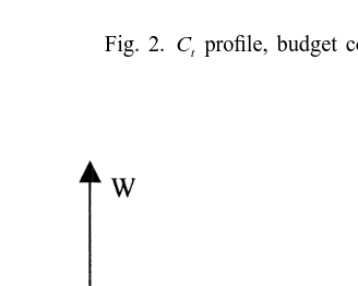
3.1.2. Lifetime resource constraint binding
The optimal consumption profile is fully characterized by the following equation:
a 21 a 21 (r 1p2r)t (r 1p2r)t (r 2r)t
Ct 5(C0 e 2b(e 2e )), (15)
combined with the binding resource / budget constraint
`
2rt
E
C et dt5W .0 (16)0
The wealth profile over time follows trivially from the above consumption process. The continuous lines in Figs. 2 and 3 illustrate consumption and wealth profiles for the case of g,0 and a value b of the bequest parameter. The dotted line in1
int
the consumption graph represents the interior solution C of the previous section for the same value of the bequest parameter.
Notice that C is smaller than what it would have been if the interior solutiont
int 1 / (a 21 )
were attainable. Indeed, C0,C0 5b because of the lower bound that the bequest motive imposes on the marginal utility of wealth. Further notice the time
~
pattern of C /C as displayed in Table 2: the consumption growth rate is strictlyt t
smaller than the growth rate (r2r) /(12a) for the interior solution.
More generally, both consumption levels and growth at any point in time are
~
increasing in W as dC / dW0 t 0.0 and d(C /C ) / dWt t 0.0. In the limit, as initial
1 / (a 21 ) ~
wealth increases, we have C0→b and C /Ct t→(r2r) /(12a), which corresponds to the consumption pattern for an interior solution.
Totally differentiating the rate of growth of consumption with respect to the
~
Fig. 2. C profile, budget constraint binding.t
Fig. 3. W profile, budget constraint binding.t
confronted with a case other than the interior solution of the previous section, the bequest motive does not only have an impact on the level of the consumption profile such as illustrated by the decrease in C , but also on the slope.0
Table 2
~
Time pattern of C /C
~
Time C /Ct t
12a
t50 [(r2r 2p) /(12a)]1[ pbC0 /(12a)] (r 2r)t 12a
t.0 [(r2r 2p) /(12a)]1[ pbe Ct /(12a)]
Proposition 1. Suppose the consumption process is determined by the equation
Proof. It is easy to derive dC / db0 ,0 using the two equations that determine the consumption path. Further, we can use the results from Table 2 and show
~
d(C /C ) / dtt t ,0 holds over the entire interval considered. Using these results
~
together with d(C /C ) / dbt t .0, we are able to establish single crossing of the two consumption profiles in the interval [0,`[. Denoting the time when these profiles
*
cross t , we find the desired result. h
Corollary 2. At any time t[[0,`[, W is strictly increasing in b.t *
This latter property trivially holds for t,t as consumption is lower at all
*
times. After t , given that the present discounted value of consumption from any
*
time t.t until infinity is bigger after the increase than before, the wealth level at
t also has to be bigger accordingly.
The result that consumption will actually rise over a positive interval of time may seem somewhat surprising. But when thinking a little more carefully about the problem, it becomes less puzzling. Indeed, the increase in the bequest parameter corresponds to a stronger desire to leave money. This is exactly what is going on here. Corollary 2 shows that, at any point in time, the wealth is strictly bigger after the increase in b. In expectation, the person thus leaves a bigger bequest.
Another way of thinking about the result of Proposition 1 is to consider the constrained optimization problem the individual faces over the time interval [0,`[. An increase in b corresponds to a decrease in the marginal utility of consumption, net of its impact on wealth levels. In particular, this is true at time 0 when optimal consumption will be lower. Now thinking at the other extreme of the impact of an increase in b on the optimal consumption level at some time close to infinity, the impact is relatively speaking much smaller because the transversality condition
2rt
limt→`W et 50 binds at infinity, both before and after the change in b. Hence the consumption profile is tilted towards later periods.
level of consumption, but not between accumulated wealth and changes in consumption. Within our setup, the claim is correct for an interior solution such as described in the previous section. But, as soon as we allow for a binding budget constraint, we find that the rate of change of consumption is correlated with wealth levels. Consumption levels are, on the other hand, not monotonic in the strength of the bequest motive.
It may be instructive to look at a graphical representation of the findings. The consumption (Fig. 2) and wealth (Fig. 3) profiles are plotted under two scenarios. The continuous lines represent the profiles that are derived for a bequest parameter
b . After an increase of the bequest parameter from b to b , the consumption and1 1 2
wealth profiles shift as described above, and we obtain the dashed curves.
3.2. Liquidity constraints
Now we study the more general case of having positive annuity income levels over an interval [E,`[. Given our definition of the income process in Eq. (8), this assumption can be summarized by YE.0. In the present section, we explicitly allow for liquidity constraints. The reason for doing so is that, in many countries, retirees are restricted in their use of old-age income as collateral in credit contracts. Hence borrowing on survival contingent claims on future resources, as represented by the annuity flow Y , is limited. In the U.S., for example, usingt
Social Security entitlements as collateral is prohibited. Hausman and Paquette (1987) find empirical evidence that these legal restrictions are actually not fully undone by the markets. These authors find that, for involuntary early-retirees, there are consumption jumps at the age of first eligibility for social security benefits. Given that cycle savers would prefer to smooth consumption over the life-cycle and hence would prefer to borrow on future social security payments, this finding can be interpreted as evidence for the presence of liquidity constraints.
Summarizing, the optimization problem reduces to expressions (7)–(10) subject to the additional set of liquidity constraints
Wt$0, ;t[[0,`[. (17)
Given the form of the income process Y and the presence of explicit liquidityt
constraints, there is a multitude of scenarios. We can classify these scenarios into three big groups using the TVC and the binding of the liquidity constraints after E:
2rt
Group 1 limt→`W et .0
2rt
Group 2 limt→`W et 50, Wt50 for some t.E 2rt
Group 3 limt→`W et 50, Wt.0;t.E
2rt
at the infinite horizon, i.e. limt→`W et .0. The second group corresponds to scenarios where wealth is run down to zero in finite time and stays at zero forever after. The third and last group consists of cases that display a binding budget constraint at infinity, but where at any given time t the wealth level is positive, hence implying that the liquidity constraints never bind. Within every one of these groups, we have different scenarios depending on when precisely liquidity constraints bind in the interval [0,`[. We consider various parameter values giving us the different scenarios. We summarize the different possible scenarios in Table 3.
In the next four subsections of this paper, we present four representative scenarios. Cases 1, 5 and 7 are the simplest possible illustrations of the three big solution groups. Case 2 allows us to illustrate the impact of having liquidity constraints bind over a first retirement period before eligibility for social security benefits. All other scenarios are straightforward extensions of these representative scenarios. For a detailed analysis thereof, see Chapter 2 of Jousten (1998).
3.2.1. Case 1: Interior solution, (r 2r) /(a 21),r, g,r, budget constraint
not binding
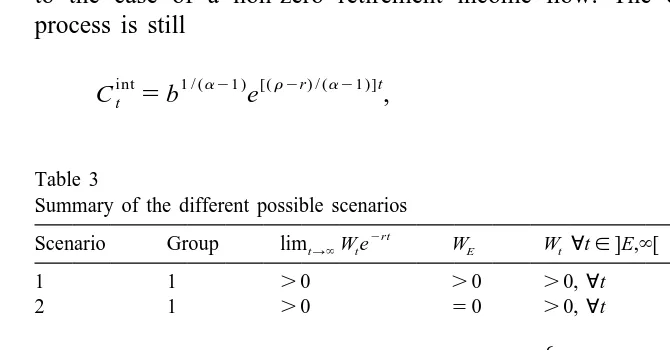
This case is the logical extension of the scenario we discussed in Section 3.1.1 to the case of a non-zero retirement income flow. The optimal consumption process is still
int 1 / (a 21 ) [(r 2r) / (a 21 )]t
Ct 5b e , (18)
Table 3
Summary of the different possible scenarios
and the comparative statics results with respect to b are also unchanged. The wealth process, on the other hand, now follows a somewhat more general process:
where V represents the annuity wealth computed using simple discounting:t
Y /(rt 2g), for t$E, Vt5
H
r(t2E )V eE , for t,E.
We know that, for this program, the financial wealth level at infinity needs to be positive. A necessary condition for this to be true is that
lim(Wt1V )t .0.
t→`
Checking this condition, we find that we have to rule out that the rate of growth of consumption levels is bigger than the interest rate, i.e. we need (r 2r) /(a 21),
r. Furthermore, we have to impose that total initial wealth is bigger than total
expected consumption:
1 / (a 21 )
W01V0.1 /hr2[(r 2r) /(a 21)]jb .
As opposed to the no-annuity case of Section 3.1.1, we also have to take the rate of growth of the annuity stream into account. To satisfy the condition that
2rt
limt→`W et .0, we need to impose that the interest rate is bigger than the rate of growth of the annuity stream (i.e., r.g). If this were not so, the second term
on the left-hand side of Eq. (19) would grow faster than the expression on the
2rt
right-hand side, with the obvious undesired effect on limt→`W et .
3.2.2. Case 2: Liquidity constraints binding at time E, (r 2r) /(a 21),r, g,
r, budget constraint not binding
A second possible solution is the one where liquidity constraints only bind at time E, but that thereafter the optimal unconstrained consumption profile is accessible. This means that for t,t[[0,E[ consumption is determined by
a 21 a 21 (r 1p2r)(t2t) (r 1p2r)t 2pt (r 2r)t
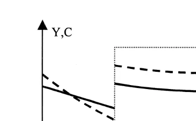
Fig. 4. C profile, constraint binding at E.t
attainable and optimal. The limiting conditions on total wealth Wt1V are alsot
12
unchanged.
To illustrate this scenario, Figs. 4 and 5 present the consumption and wealth profiles.
Notice that Eq. (20) linking the different consumption levels at all times t over the interval [0,E[ is exactly the same as the one we displayed in Section 3.1.2 for the case of a binding resource constraint in the absence of liquidity constraints.
~
Hence, the time pattern of C /C is still correctly described by Table 2.t t
The comparative statics analysis of the impact of an increase in the bequest parameter b is of course somewhat more complicated in the present case than it was for an interior solution. For the part of the profile that is unconstrained, i.e. all times t$E, the comparative statics result (14) obviously still holds. On the
Fig. 5. W profile, constraint binding at E.t
12
The conditions are (r 2r) /(a 21),r, g,r and total initial resources bigger than total expected
interval [0,E[, however, the analysis differs and resembles Proposition 1 of Section 3.1.2.
Proposition 3. Suppose we have a bounded interval of time [t ,t [where the
1 2
consumption process is determined by the equation
a 21 a 21 (r 1p2r)(t2t) (r 1p2r)t 2pt (r 2r)t
that determine the consumption path. Further, using the expression for C /C fromt t
~ ~
Table 2 we know d(C /C ) / dtt t ,0 and d(C /C ) / dbt t .0. Hence, we are able to establish single crossing of the two consumption profiles in the interval [t ,t [.1 2
*
Denote t the time when these two consumption profiles cross. h
Corollary 4. At any time t[[t ,t [, W is strictly increasing in b.1 2 t
The intuition for the tilt in the consumption profile is easy to understand. As b increases, the value the individual attaches to bequests increases much more at time t rather than at some time t close to t . The reason is that the individual1 2
knows that he runs down wealth to zero until time t . Hence, to make the budget2
constraint hold, a decrease in consumption early in retirement has to be compensated by an increase in consumption later in life.
Using Proposition 3 for the special case where t150 and where t25E, we can
summarize our findings by
or perhaps even more instructively in Fig. 6, where the dashed line describes the consumption profile under the initial value of the bequest parameter b and the1
continuous line describes the consumption profile under the new increased value of the parameter b .2
Fig. 6. Effect of b on consumption profile.
3.1.2 that Bernheim et al.’s claim only holds as long as both liquidity constraints and the budget constraint are slack over the entire life-span we consider.
The present scenario is an interesting illustration of the impact of liquidity constraints on the consumption and wealth accumulation behavior of early retirees. Recalling our interpretation of the time E as the time the (early) retiree becomes eligible for social security benefits, we find that binding credit constraints, which are especially stringent for involuntary early retirees, decrease both the level and the rate of change of consumption during the earliest periods of early retirement. Further, we find that the jump in consumption at the age of eligibility should be stronger for people with smaller bequest motives.
3.2.3. Case 5: Budget constraint binding at infinity, (r 2r) /(a 21).g.(r 1
p2r) /(a 21)
2rt
After these two cases where limt→`W et .0, the next two sections contain scenarios where the latter expression is 0. It is trivial to show that, for this to be
13
true, we need (r 2r) /(a 21).g.
In the present section, we consider a growth rate of the annuity stream that is bigger than the limiting growth rate of the constrained consumption path as t→`, but smaller than the growth rate displayed for an interior solution, i.e. (r 2r) /
(a 21).g.(r 1p2r) /(a 21). Denoting T (.E ) the time when the liquidity
constraints start to bind, the optimal consumption path is determined by
a 21 (r 1p2r)t (r 1p2r)t (r 2r)t 1 / (a 21 )
(C0 e 2b(e 2e )) , for t,T, Ct5
H
Y ,t for t$T,
] 13
Suppose the latter relation does not hold. Then there exists a time t such that the optimal ] unconstrained consumption profile and the annuity income profile will cross, hence implying for t.t a
Fig. 7. C profile, constraint binding at tt .E.
combined with the resource constraint
T
2rt W05
E
(Ct2Y )et dt.0
Further, given the concavity of the utility function, it can easily be shown that consumption will be continuous in time
a 21 (r 1p2r)T (r 1p2r)T (r 2r)T 1 / (a 21 ) g(T2E )
(C0 e 2b(e 2e )) 5e Y .E
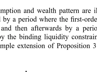
The consumption and wealth pattern are illustrated in Figs. 7 and 8. They are characterized by a period where the first-order conditions determine the consump-tion profile, and then afterwards by a period when the consumpconsump-tion pattern is determined by the binding liquidity constraints.
Using a simple extension of Proposition 3 it is easy to derive the comparative
**
statics of the consumption path as we vary b: there is a time t [[0,E[ and a point in time T9 .T such that
binding liquidity constraint at E. The results we derive in this scenario closely parallel those we found in Section 3.1.2 when discussing the optimal consumption and wealth profiles for a binding lifetime resource constraint in the absence of annuitized income. Indeed, we find that the optimal consumption profile is determined by Eq. (20) as well as the binding budget constraint
`
2rt
E
(Ct2Y )et dt5W .0 0Notice that the present scenario is most plausible for a constant nominal annuity stream ( g,0), which is the standard in private pension arrangements in the U.S. Indeed, for a constant real annuity stream ( g50) we would have to impose the rather implausible requirement r.r 1p to be in the present scenario. For g,0, on the other hand, the condition (r 1p2r) /(a 21).g becomes much more
plausible, especially for risk averse individuals.
3.3. Comments on the uncertainty case
We conclude this section by summarizing our results. First, the consumption level at any time t can be determined by three regimes: an interior solution, a first-order condition combined with a binding budget constraint and the exogenous retirement income level.
Second, a finding that the reader may not have suspected at the outset is that consumption levels actually increase with the strength of the bequest motive over some subintervals in all cases except the one when the optimal unconstrained consumption path can be attained. The intuition for this result is that the consumption profile changes slope on constrained intervals, and therefore forces a reallocation of resources from earlier periods to later periods, as consumption in earlier periods becomes relatively speaking less interesting due to the increased opportunity cost in terms of foregone bequests. By doing so, the slope of the consumption profile approaches the slope of the optimal unconstrained
consump-~
tion profile (r2r) /(12a), a fact that is captured by the expression d(C /C ) /t t
db.0.
consumption levels in periods when the consumption process is determined by an interior solution, it is easy to see that increases in the bequest parameter b render liquidity constraints less binding. An intuitive way to see this general result is to look at the special case of Section 3.2.2. There was a jump in consumption at the age of first eligibility for retirement benefits because of binding borrowing constraints over the early retirement period. As we increase the value of the bequest parameter b, the discontinuity in consumption shrinks, as can easily be seen in Fig. 6. The mechanism behind this reduction is that the person attaches a smaller value to consumption early in life, hence reducing the implicit cost of not being able to borrow on the future. Therefore, for a sufficiently high b, we will end up in the case of the interior solution determining consumption over the entire life-span.
Notice that the effect on the wealth profile as we increase the bequest parameter is exactly as expected, as the wealth and thus bequests grow in expectations and, even more strongly, it is non-decreasing at any given point in time.
4. Annuity valuation
Using the setup of Section 3, we analyze the question of annuity valuation. The previous literature has largely ignored the impact of bequest motives on the value of annuities. There have been two common approaches to computing the value of an annuity payout stream. A first strand of the literature relies on simple actuarial calculations. It is easy to show that this method is correct in the case of either a risk averse consumer or a competitive annuity market. The second approach is due to Bernheim (1987). Using a standard life-cycle model with a risk averse individual and a marginal unavailability of annuities, Bernheim showed that the value of an annuity is close to the simple financial value of the annuity payout stream. The reason for this finding is easiest to understand when comparing a survival contingent annuity contract to a simple financial asset. Without binding liquidity constraints, an individual attaches equal value to an annuity contract paying out $1 every period conditional on survival and a financial asset paying out $1 per period independently of survival. Hence, annuities should be valued exactly in the same way as a financial asset.
Following the typology of Table 3 of Section 3.2, we can once again discuss annuity valuation within every one of the eight possible scenarios. In the present section we only analyze the same four representative scenarios that we presented
14
in Section 3.2.
14
4.1. Case 1: Interior solution, (r 2r) /(a 21),r, g,r, budget constraint not
binding
In this particular setup, it is easy to determine the value of the marginal dollar of annuity payments Y in terms of financial wealth at time 0 (W ):E 0
2(r1p)E
dW0 e
]]
*
5 2]]]. dYE U* r1p2gRecalling the definition of the simple discounted value of annuity wealth V fromt
Section 3.2.1, we can also rewrite the present finding as
dW0 r2g 2pE
]]
*
5]]]e . dV0 U* r1p2gact
Similarly, defining the actuarially correctly discounted value of annuity wealth Vt
as the present discounted value, taking both survival probabilities and interest rates into account: for the marginal value of annuity payouts as
dW0
]]act
*
5 21.U
dV0 *
This result stands in stark contrast to Bernheim’s finding that, for the case of no binding liquidity constraints, the correct way to discount future annuity payouts is to use simple discounting and not the actuarially correct counterpart. The reason for this quite dramatic change is that the individual no longer only attributes a certain utility value to the periods when alive, but also to the periods when dead. This implies that annuities and financial assets are no longer perfect substitutes and he values a financial asset more since it pays out a return in every future state of the world, whereas the annuity only pays out a return in the states when the individual is alive.
The result also means that we do not need to have perfect annuity markets or a coefficient of relative risk aversion equal to zero to validate actuarially fair valuation. It suffices to have an interior solution for a risk averse consumer with a bequest motive, and this independently of the existence of a market in marginal annuity claims. The reason for this finding is that the equalization of marginal utilities of consumption and bequests in all possible states of the world makes the individual de facto risk neutral.
example, another natural way to look at the same problem of marginal annuity valuation is to look for the change in period E financial wealth required to keep the person indifferent after a marginal change of annuity holdings. Notice that, to make this comparison meaningful, we need to assume that the individual cannot borrow against period E wealth. More formally, we are interested in the value of
act
(dW / dVE E )uU*.
For the case of our interior solution, it is trivial to show that
dWE dW0
]]act
*
5]]act*
5 21,U U
dVE * dV0 *
and hence that the two approaches prove to be totally identical. Further, the restriction of considering wealth at period E that the person cannot borrow against is not a real restriction for the case of an interior solution since wealth levels are anyway positive at all times.
4.2. Case 2: Liquidity constraints binding at time E, (r 2r) /(a 21),r, g,r,
budget constraint slack
As noted in Section 3.2.2, the present case best describes the situation of an early retiree whose consumption is constrained before the time of first entitlement (E ) to retirement benefits, but who attains the optimal unconstrained consumption levels after E. The value of an increase of a marginal dollar of annuity payout YE
in terms of the period 0 concepts is
dW0 1 individual attributes to the annuity payout stream Y is inferior to the actuarialt
value.
This latter result is rather interesting as it shows that, for people facing binding liquidity constraints in their early periods of life, even an actuarially fair insurance system would not be sufficient to have them participate in the annuity market. But the finding is not surprising. First the payout stream does not have an annuity
value, i.e. there is no bigger utility attached to receiving income when alive rather
additional resources in the unconstrained interval after initial entitlement E. Similarly, we can say that any deterministic future payment displays the same property. Indeed, comparing a $1 state-of-the-nature independent payout in period
E to its compensating variation in terms of W , we also find that the latter is0
2rE
smaller than e because of the binding liquidity constraint for the time period [0,E[. To separate out the part of the effect that is due to the inherent survival-contingent characteristics of annuities, we use our second measure of annuity valuation, which is based on the wealth concepts as of age E, supposing it is impossible to borrow on W . Computing the latter, we findE
dWE
]]act
*
5 21,U
dVE *
which means that the net effects due to the annuity’s inherent characteristics are not changed with respect to the previous scenario of a fully interior solution.
4.3. Case 5: Budget constraint binding at infinity, (r 2r) /(a 21).g.(r 1
p2r) /(a 21)
Recalling our findings from Section 3.2.3 on the consumption and wealth profiles, we know that liquidity constraints bind from some finite time T onwards. Hence, after time T, the value of the annuity stream will be smaller than the actuarially fair value.
It is difficult to derive the value of a marginal annuity stream explicitly. Nonetheless, we can derive rough bounds on its value:
dW0 ]]
0.
*
. 21. dV0 U*Without any additional information on the precise parameter values of the problem, it is difficult to determine whether the value of the marginal annuity is bigger or smaller than the actuarial value, as there are two effects playing in opposite directions. Prior to time T, there is a clear annuity value to having this payout stream rather than a financial asset of the same actuarial value. After T, the annuity payout stream generates a utility which is lower than the one generated by a financial asset, as the individual would prefer to reallocate annuity income which is possible in the case of financial wealth.
4.4. Case 7: Budget constraint binding at infinity, (r 1p2r) /(a 21).g
dW0
The value of an annuity is hence bigger than its actuarial value, but still smaller than the purely financial value. This result is quite intuitive: because of the binding budget constraint, there is a clear annuity value attached to the retirement income stream. The above finding is reconfirmed when we look at the bounds that we can impose on the expression (dW / dV )E E uU*. We can easily determine that
dWE r2g
]] ]]]
21,
*
, 2 .dVE U* p1r2g
4.5. Summary of the annuity results
Our results show that Bernheim’s (1987) claim that the value of an annuity is close to the simple discounted value of future payouts has to be nuanced. Indeed, for a sufficiently strong bequest motive, even in the presence of a marginal unavailability of annuity contracts and without perfect competition, actuarial valuation is the better method for valuing future annuity claims. Our analysis shows that the use of an actuarially correct valuation in the presence of imperfect annuity markets implicitly assumes an active bequest motive. Simple financial valuation, on the other hand, implicitly assumes no bequest motive.
When allowing for an early retirement phase from time 0 to E, we show that to separate the value of the annuity stream that is due to the survival-contingency from the value that is due to the binding of the liquidity constraints during the early retirement period, we should use a second indicator. We use wealth at the time of first entitlement E that we cannot borrow against in addition to the standard period 0 wealth equivalence measure such as used by Bernheim.
5. Conclusion
valuation of marginal annuity claims. Using a quasi-linear approach to analyze these questions we successively studied the simplest two-period certainty case as well as the infinite horizon life-span uncertainty model.
Within the framework of the first model, we have a clear result that consump-tion is monotone non-increasing in the linear bequest parameter, and that wealth is hence monotone non-decreasing. Switching over to the life-span uncertainty case, we showed that the above result no longer holds, except in the case of a strictly interior solution. Indeed, as soon as liquidity constraints or the budget constraint bind, there is a strictly positive interval of time during which consumption actually rises! As surprising as this result may seem, we show that it is just the natural complement of the finding that an increased bequest motive generates higher wealth levels at any point in time.
We further show that, as long as liquidity constraints or the budget constraint are binding at some point in time, a bequest motive does not only affect consumption levels, but also the slope of the consumption profile. The latter effect of a bequest motive on the slope has generally been ignored. This monotone effect of the bequest parameter on consumption growth rates gives a clear way of testing for the validity of the model.
As for annuity valuation, our analysis shows that there is no single criterion that completely summarizes the value of a marginal annuity payout stream to the individual. Using two different, but closely related, concepts of valuation, we are able to separate out the pure annuity effect from the additional effect due to the timing of the onset of the annuity payout stream. We show that as soon as we deviate from the simplest life-cycle framework with uncertainty such as the one used by Bernheim (1987), the value of a marginal increase payout is no longer equal or very close to the present discounted value computed using simple discounting, but tends towards the direction of its actuarially correct equivalent. We find that for the case of a sufficiently strong bequest motive, actuarial valuation is closest to the true economic value of a marginal annuity stream. For a weak or non-existent bequest motive, simple financial discounting best approximates the true value. These findings are important for some of today’s most acute policy questions, particularly the evaluation of reforms to the present-day old-age income systems. To evaluate and understand the changes to the system, there is a need to correctly measure the value of future annuity payouts. Our findings indicate that, depending on the scenario we are in, using simple financial discounting for valuing future social security and pension may introduce a major measurement error into the analysis.
Acknowledgements
`
Liege for their helpful comments. Thanks are also due to two anonymous referees for their suggestions. All remaining errors are entirely my own.
References
Bernheim, B.D., 1987. The economic effects of social security. Journal of Public Economics 33 (3), 273–304.
Bernheim, B.D., Skinner, J., Weinberg, S., 1997. What accounts for the variation in retirement wealth among U.S. households? Mimeo.
Coile, C., Diamond, P., Gruber, J., Jousten, A., 1999. Delays in claiming social security benefits. NBER Working Paper No. W7318.
Fischer, S., 1973. A life cycle model of life insurance purchases. International Economic Review 14 (1), 132–152.
Friedman, B.M., Warshawsky, M., 1988. Annuity prices and savings behavior in the United States. In: Bodie, Z., Shoven, J.B., Wise, D.A. (Eds.), Pensions in the U.S. Economy. NBER and University of Chicago Press, Chicago, pp. 53–84.
Hausman, J.A., Paquette, L., 1987. Involuntary early retirement and consumption. In: Burtlees, G. (Ed.), Work, Health and Income Among the Elderly. The Brookings Institution, Washington, DC, pp. 151–181.
Hurd, M.D., 1989. Mortality risk and bequests. Econometrica 57 (4), 779–813.
Jousten, A., 1998. Essays on annuity valuation, bequests and social security. PhD thesis, MIT. Yaari, M.E., 1965. Uncertain lifetime, life insurance, and the theory of the consumer. Review of