23 11
Article 10.6.7
Journal of Integer Sequences, Vol. 13 (2010), 2
3 6 1 47
Generalized
j
-Factorial Functions,
Polynomials, and Applications
Maxie D. Schmidt
University of Illinois, Urbana-Champaign
Urbana, IL 61801
USA
Abstract
The paper generalizes the traditional single factorial function to integer-valued mul-tiple factorial (j-factorial) forms. The generalized factorial functions are defined recur-sively as triangles of coefficients corresponding to the polynomial expansions of a subset of degenerate falling factorial functions. The resulting coefficient triangles are similar to the classical sets of Stirling numbers and satisfy many analogous finite-difference and enumerative properties as the well-known combinatorial triangles. The generalized triangles are also considered in terms of their relation to elementary symmetric poly-nomials and the resulting symmetric polynomial index transformations. The definition of the Stirling convolution polynomial sequence is generalized in order to enumerate the parametrized sets of j-factorial polynomials and to derive extended properties of thej-factorial function expansions.
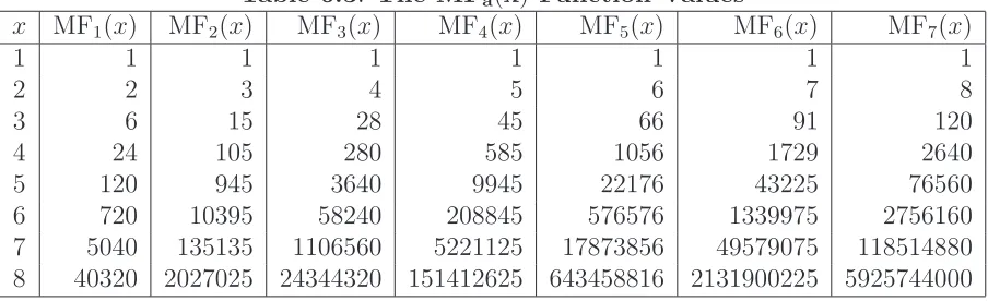
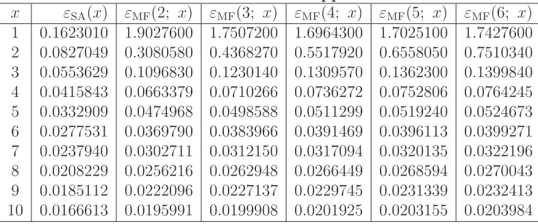
The generalized j-factorial polynomial sequences considered lead to applications expressing key forms of thej-factorial functions in terms of arbitrary partitions of the j-factorial function expansion triangle indices, including several identities related to the polynomial expansions of binomial coefficients. Additional applications include the formulation of closed-form identities and generating functions for the Stirling numbers of the first kind and r-order harmonic number sequences, as well as an extension of Stirling’s approximation for the single factorial function to approximate the more generalj-factorial function forms.
1
Notational Conventions
number triangles and the Stirling polynomial sequences [24; 32] are used to denote these forms and reasonable extensions of these conventions are used to denote the generalizations of the forms established by this article. The usage of notation for standard mathematical functions is explained inline in the text where the context of the relevant forms apply [46]. The following is a list of the other main notational conventions employed throughout the article.
• Indexing Sets: The natural numbers are denoted by the set notation N and are
equivalent to the set of non-negative integers, where the set of integers is denoted by the similar blackboard set notation for Z. The standard set notation for the real
numbers (R) and complex numbers (C) is used as well to denote scalar and approximate
constant values.
• Natural Logarithm Functions: The natural logarithm function is denoted Log(z) in place of ln(z) in the series expansion properties involving the function. Similarly Log(z)k denotes the natural logarithm function raised to thekth power.
• Iverson’s Convention: The notation [condition]δ for a boolean-valued input con-dition represents the value 1 (or 0) where the input concon-dition evaluates to True (or
False). Iverson’s convention is used extensively in theConcrete Mathematics reference and is a comparable replacement for Kronecker’s delta function for multiple pairs of arguments. For example, the notation [n=k]δ is equivalent to δn,k and the notation [n=k= 0]δ is equivalent to δn,0δk,0.
• Sequence Enumeration and Coefficient Extraction: The notation
hgni 7→ {g0, g1, g2, . . .}denotes a sequence indexed over the natural numbers. Given
the generating function F(z) representing the formal power series (also generating series expansion) that enumerateshfni, the notation [zn]F(z) :=fn denotes the series
coefficients indexed by n∈N.
• Fixed Parameter Variables: For an indexing variable n, the notation Nc is em-ployed to represent a fixed parameter in a formula or generating function that is treated as a constant and that is only assigned the explicit value of the respective non-constant indexing variable after all other variables and indices have been input and processed symbolically in a relevant form. In particular the fixed Nc variable should be treated as a constant parameter in series or generating function closed-forms, even when the non-constant form of n refers to a particular coefficient index in the series expansion. The footnote on p.18clarifies the context and particular utility of the fixed parameter usage in a specific example inline in the text.
2
Introduction
The parametrized multifactorial (j-factorial) functions studied in this article generalize the standard classical single factorial [A000142] and double factorial [A001147; A000165; and
A006882] functions and are characterized by the analogous recursive property in (2.1).
The classical generalized falling factorial function, (z|α)n , studied extensively by Adelberg
and several others [3; 15;16; 28; 35; 64], can be defined analytically in terms of the gamma function in (2.2) and by the equivalent product expansion form in (2.3). The function can also be expressed by the equivalent finite-degree polynomial expansion in z with coefficients given in terms of the unsigned triangle of Stirling numbers of the first kind [A094638] in equation (2.4).
(z|α)n := α
n Γ(z α)
Γ(αz −n) + [n = 0]δ (2.2)
=
n−1
Y
i=0
(z−iα) + [n= 0]δ (2.3)
=
n
X
k=1
n k
(−α)n−kzk+ [n = 0]
δ (2.4)
The definitions of (2.2) and (2.3) extend a well-known simplified case of thefalling factorial
function for α = 1, commonly denoted by the equivalent forms xn = x!/(x−n)! and (x) n
[24; 50]. Other related factorial function variants include the generalized factorials of t of order n and increment h, denotedt(n, h), considered by C. Charalambides [17, §1], the forms
of theRoman factorial and Knuth factorial functions defined by Loeb [40], and the q-shifted factorial functions defined by McIntosh [42] and Charalambides [17, (2.2)].
This article explores forms of the polynomial expansions corresponding to a subset of the generalized, integer-valued falling factorial functions defined by (2.3). The finite-difference forms studied effectively generalize the Stirling number identity of (2.4) for the class of degen-erate falling factorial expansion forms given by (x−1|α)n whenα is a positive integer. The
treatments offered in many standard works are satisfied with the analytic gamma function representation of the full falling factorial function expansion. In contrast, the consideration of the generalized factorial functions considered by this article is motivated by the need for the precise definition of arbitrary sequences of the coefficients that result from the variations of the finite-degree polynomial expansions inz originally defined by equation (2.4).
For example, in a motivating application of the research it is necessary to extract only the even powers ofz in the formal polynomial expansion of the double factorial function over
z. The approach to these expansions is similar in many respects to that of Charalambides’ related article where the expansion coefficients of the generalized q-factorial functions are treated separately from the forms of the full factorial function products [17, §3 and §5]. The coefficient-based definition of the falling factorial function variants allows for a rigorous and more careful study of the individual finite-degree expansions that is not possible from the purely analytic view of the falling factorial function given in terms of the full product expansion and infinite series representations of the gamma function [cf. (2.2)].
in§4, and in the forms of the j-factorial polynomials that generalize the sequence of Stirling polynomials in§5. A number of interesting applications and examples are considered as well, with particular emphasis on the forms discussed in §4.3 and §6.
3
Finite Difference Representations for the
j
-Factorial
Function Expansion Coefficients
3.1
Triangle Definitions
Consider the coefficient triangles indexed overn, k ∈Nand defined recursively by equations
(3.1) and (3.2) [35, cf. (1.2)].
n k
α
= (αn+ 1−2α)
n−1
k
α
+
n−1
k−1
α
+ [n=k= 0]δ (3.1)
n k
α
= (αk+ 1−α)
n−1
k
α
+
n−1
k−1
α
+ [n=k = 0]δ (3.2)
The “triangular” recurrences defining the α-factorial triangles are special cases of a more general form in equation (3.35) that includes well-known classical combinatorial sets [24, Ch. 6] such as the Stirling cycle numbers (first kind) [A008275; and A094638], also defined by (3.1) when α := 1, the Stirling subset numbers (second kind) [A008277], the Eulerian numbers for permutation “ascents” [A066094], and the “second-order” Eulerian numbers
[A008517] [cf.§6.2.4]. The unsigned triangles corresponding to a positive integer parameter
αare unimodal over each row and are strictly increasing at each fixed column for sufficiently large row indexn [62, §4.5]. The signed coefficient analog of the triangle in (3.1) is defined recursively as (3.3) and may be expressed in terms of the unsigned triangle by the conversion formulas in equation (3.4).
n k
α
= (2α−αn−1)
n−1
k
α
+
n−1
k−1
α
+ [n =k = 0]δ (3.3)
n k
α
= (−1)n−k
n k
α
⇐⇒
n k
α
= (−1)n−k
n k
α
(3.4)
The implicit interpretation of the (3.1) triangle as expansion coefficient sets is demon-strated by considering the motivation for the following procedure. Let the polynomialpn(x) correspond to the nth distinct polynomial expansion of the α-factorial function, (x−1)!
(α),
and define the polynomial coefficients as [xk−1]pn(x) := n k
α. Observe that provided a
polynomial (row) indexn, the coefficient forms corresponding to subsequent polynomial ex-pansions are formed by the multiplication of a linear factor inxwith the existing polynomial. The next equation defines the triangle of coefficients that result from the expansions of this form [17, cf. Thm. 3.2].
[xk−1]pn(x) = (αn+ 1
−2α) [xk−1]pn
It follows that for rows indexed byn ∈[1, ∞)⊆Nand columns indexed byk ∈[1, ∞)⊆N,
the polynomial expansions yield an identical recursive definition of theα-factorial coefficient triangles to that given by (3.1) [cf. (3.5)].
In order to evaluate the factorial function expansions numerically, consider that the range of natural numbers that correspond to any distinctα-factorial polynomial expansion ins is a function ofα: there is exactly onen ∈N for each single factorial function expansion, two
n∈N for each double factorial function expansion, and so on for each positive integer value
of α.
3.2
Finite-Difference Properties
Many analogs of the classical Stirling number identities and related combinatorial properties for the triangles in equations (3.1) and (3.2) are generalized by the analogous forms in the following discussions [cf. §3.4.2]. A number of additional identities and forms related to the Stirling number forms, including relations to the Bell numbers [A000110], Lah numbers
[A008297],multi-poly Bernoulli numbers, andTanh numbers [A111593], are discussed in the references by Agoh and several others [9; 8; 10; 47] [16, (3.5)] [24, Table 202] [26, §2 and
§3] [28, §3.1] [55, Thm. 2.1 and (2.4)]. The discussions and properties of the α-factorial polynomials given in §5 also provide a number of identities involving generalized Bernoulli polynomials and other functions that may be applied to the forms of (3.1) and (3.2). The next section in§4 contains detailed discussions of the (3.1) triangle properties as well.
The initial characteristic finite-difference properties defining the Stirling number sets are mirrored by the generalizedα-factorial triangles as given by the following equations in (3.5) and (3.6) [34, §1.2.6].
(x−1|α)n =
n−1
X
k=0
n k+ 1
α
(−1)n−1−kxk (3.5)
xn :=
n
X
k=0
n k
α
(x−1|α)k (3.6)
Depending on the application it may be convenient to define the parameter α in equations (3.1) and (3.2) over the rational numbers. This slight generalization in form will still result in the correct form for the interpretation given by the product expansion of (3.5). For example, the book Concrete Mathematics considers the form of rk(r−1/2)k related to the
central binomial coefficients [24, §5.3]. One additional special case of equation (3.1) occurs when α := 0 where the form provides the recursive definition for Pascal’s triangle. The case degrades nicely in the context a 0-factorial function where the polynomial factors in the expansion remain constant in form over all n. The form of equation (3.5) for this case then effectively defines the binomial theorem in reverse: Pknk0 sk−1 = (s+ 1)n−1.
equations (3.7) and (3.8). n X k=0 n k α k m α
(−1)n−k = [m =n]
δ (3.7) n X k=0 n k α k m α
(−1)n−k = [m =n]
δ (3.8)
The orthogonality relation for the Stirling numbers is preserved in these properties for the generalized triangles and defines the analogous result of corollary (3.9) [47, cf. (1.1)] [24].
f(n) =
n X k=0 n k α
(−1)kg(k) ⇐⇒ g(n) =
n X k=0 n k α
(−1)kf(k) (3.9)
The identities of equations (3.10) and (3.11) generalize classical Stirling number proper-ties as well [24, Table 265].
n
X
k=0
n+ 1
k+ 1
α k m α
(−1)m−k = αn
−m Γ n+ 1
α
Γ m+ 1
α
[n ≥k]δ (3.10)
n+1
X
k=0
n+ 1
k+ 1
α k m α
(−1)m−k = n−k
X
j=0
k−1 +j k−1
αj+ [k= 0]δ (3.11)
The generalized first triangle in (3.1) can be expressed in terms of the Stirling numbers of the first kind through the following identities.
n k α =
n−k
X
j=0
n−1
k−1 +j
k−1 +j k−1
αn−k−j + [n =k= 1]
δ (3.12)
x x−n
α = n X k=0 x x−k
αk Γ(x−k) (1−α)n−k
Γ(x−n) Γ(n−k+ 1)
The generalized second triangle in (3.2) can be expressed in terms of the Stirling numbers of the second kind through the following equations [8, (3.4) and (3.5)].
n k α =
n−k
X
j=0
k−1 +j k−1
n−1
k−1 +j
αj (3.13)
=
k−1
X
i=0
n−k
X
j=0
n−1
k−1 +j
k−1
i
(−1)i αj (k−1−i)k−1+j
(k−1)!
=
k−1
X
i=1
n−k
X
j=0
n−1
k−1 +j
k−2
i−1
(−1)k−1+i αj ik−2+j
(k−2)!
Let the linear differential operator, {Dk}[f(Nc)], be defined such that for integer k ≥ 1
{Dk}[f(N
c)] := f(Nc) [k = 0]δ. Additional properties of the generalized first triangle are
then given in pairs below for the finiten →Nc and corresponding finite-difference“binomial derivative” formulas. n k α =
Dk−1
(k−1)!αk−1 +
Dk−2
(k−2)!αk−2
"Xn−3
i=0
(αNc+ 1−2α)i+1(−α)n−3−i
n−2
i+ 1
#
=
n−3
X i=0 i+1 X r=0
n−2
i+ 1
i+ 1
r
r k−1
(−1)n−3−iαn+r−2−i−kNr+1−k
c (1−2α)i+1
−r
(3.14)
+
n−3
X i=0 i+1 X r=0
n−2
i+ 1
i+ 1
r
r k−2
(−1)n−3−iαn+r−1−i−kNr+2−k
c (1−2α)i+1
−r n k α =
Dk−1
(k−1)!αk−1 +
Dk−2
(k−2)!αk−2
"Xn−2
i=0
(αNc+ 2−2α)i(−1)n−i
n−1
i+ 1
α
#
=
n−2
X i=0 i X r=0
n−1
i+ 1
α i r r k−1
(−1)n−iαr+1−kNr+1−k
c 2i
−r(1
−α)i−r (3.15)
+
n−2
X i=0 i X r=0
n−1
i+ 1
α i r r k−2
(−1)n−iαr+2−kNr+2−k
c 2i
−r(1
−α)i−r
The second of the listed “binomial derivative” formulas may be considered as an “involution of sorts” since the coefficient form of nkα is given in terms of coefficients from the same triangle. The identity is also of particular interest since the involution-like phrasing results in the applications for the α-factorial polynomials discussed in §5.3.2 and §5.3.4 that are based on the alternate forms of the involution identities derived in §4.2.1.
Finally, the sums of the first coefficient triangle rows indexed over the integern≥1 have the generalized forms given by the next pair of equations in (3.16) and (3.17) [24, cf. (6.9)]
n X k=0 n k α
=αn−1 Γ n−1 + 2
α
Γ α2 (3.16)
n X k=0 n k α
(−1)n−k = n X k=0 n k α
= 0 (3.17)
3.3
Enumerative Properties
To begin with, consider the next generalization of the classical identity of (3.18) [24, (7.48)] in equation (3.19) defined over the upper indexm∈[1, ∞)⊆N.
X
n≥0
m n
zn =zm =z(z+ 1)· · ·(z+m−1) (3.18)
X
n≥0
m n
α
zn−1 = α
m−1Γ(m−1 + z+1
α )
Γ(z+1
α )
(3.19)
Next, let the function fm be defined by equation (3.20).
fm := m X k=0 k X j=0 j X i=0 m k α k j
j+ 1
i+ 1
(−α)k−j i! zi
(1−z)i (3.20)
The form of the identity in equation (3.21) [24, (7.46)] can be extended by the forms of (3.22) and (3.23), as well as by the form of equation (3.24) for positive integer m [3] [22, cf.
Ak,i].
∞
X
n=0
nm zn =
m X k=0 m k
k! zk
(1−z)k+1 (3.21)
∞
X
n=0
(n−α+ 1)m zn =
m
X
k=0
[(1−z)k+1]fm +1
(k+ 1) (1−z)k+1 (3.22)
∞
X
n=0
(n−α+ 1)m zn =
m
X
j=1
m m+ 1−j
1/α
(−α)j−1(m−j)!
(1−z)m+1−j (3.23)
∞
X
n=0
(αn+β)m zn =
∞ X n=0 m X k=0 m k
αkβm−knk
!
zn (3.24)
The classical “double” generating functions enumerating the original Stirling number trian-gles are defined by the following forms as [24, (7.54) and (7.55)]
∞ X m=0 ∞ X n=0 n m
wmz n
n! =e
w(ez−1)
and ∞ X m=0 ∞ X n=0 n m
wmz n
n! = 1 (1−z)w
and yield the generalizations to theα-factorial triangle cases given in respective order by the next equations in (3.25) and (3.26).
∞ X m=0 ∞ X n=0 n m α
wmzn
(n−1)! =wze
z ew(eαz−1)/α
−1 (3.25)
∞ X m=0 ∞ X n=0 n m α wmzn
n! =
(1−αz)−(w+1)/α
(α−w−1) (α−1)(1−αz)
(w+1)/α+w(αz
It follows from equation (3.26) that for m, n≥1 and for all k ∈N, the results of equations
(3.27) and (3.28) hold for the generalized triangle coefficients [cf.§6.1].
m X k=1 n k α sk−1
n! = [w
mzn]
(1−zα)
−1+αsw (α
−1)(1−zα)1+αsw −sw(1−αz)
s(w−1)(1−α+sw)
(3.27) n X k=1 n k α sk−1
n! = [z
nwk]
1−
αz w
−1+sw
α w 1− αz w
1+sw
α +αz−w
(w−1)(1−α+sw)
(3.28)
The result of the identity in (3.28) corresponds to the coefficients on a prescribed diagonal index of the full generating function in equation (3.27) [54, cf. §6.3]. Both of the identities are related to theα-factorial function expansion polynomial properties discussed in §6.1.
A generalization of the classical identity in (3.29) [24, (7.49)] can be derived from the form of (3.13) and is given by equation (3.30).
∞ X n=0 n m zn n! =
(ez−1)m
m! (3.29)
∞ X n=0 n m α zn
(n−1)! =
α1−m
(m−1)! ze
z(eαz−1)m−1 (3.30)
It can be shown from equation (3.15) that for positive m ∈ N the following identity holds
where the α-factorial polynomialσα
n(x) is defined formally in§5.2.1.
(m−1)! (n−1)!
n+ 1
m
α
=
n−1
X i=0 i X r=0
(−1)n−1−iσα
n−1−i(Nc)αr+1−m(Nc+ 1)r+1−m(2−2α)i−r
(r+ 1−m)! (i−r)!
×
×
1 + α(Nc+ 1)(m−1) (r+ 2−m)
The identity provides the alternate generating function form for the analog of equation (3.31) [24, (7.50)] given in equation (3.32).
∞ X n=0 n m zn n! =
1
m!Log
1 1−z
m (3.31) ∞ X n=0
n+ 1
m
α zn
(n−1)! =
(m−1 +z) (m−1)! z
m−1ez
αzeαz eαz−1
Nc
(3.32)
An alternate extension of (3.31) [24, (7.50)] is given by equation (3.33) and is derived from the forms in (5.24) and (5.25) wheret := 1 and S1(αz) =−Log(1−αz)/(αz) [cf. §5.3.5].
∞ X n=0 n m α zn n! =
∞ X n=0 n X k=0
(−1)m+k Log(1−αz)m+k (1−α)k αm+k (m+k)k! (m−1)!
!
3.4
Relations to Generalized Stirling Numbers
The triangles defined in §3.1 may be compared to several of the treatments given in the referenced literature on Stirling numbers and the related properties of single factorial func-tion expansions. Particular generalizafunc-tions and variafunc-tions on the classical Stirling number triangles are discussed in the references by Adelberg and others [11; 30; 44; 43] [3, §7] [16,
§3 and §4] [35, §1.3 and §2.4; cf. §3.1] [58, §4, (5.23), and (5.24)] [64, §3]. Combinatorial interpretations and examples for thegeneralized Stirling number sets are discussed elsewhere by Lang [37]. Additionally, several Stirling number forms and properties are defined in terms of the differences of more generalized factorial functions in the work by Charalambides and Koutras [15,§4].
3.4.1 Finite-Difference Properties of the Non-Central Stirling Numbers
The form of thenon-central Stirling numbers of the first kind is discussed in Koutras’ work [35, §1]. This section explores analogous properties of the (3.1) triangle for the non-central Stirling numbers of the first kind. The properties given for the row sums of the non-central triangles [35, Remark 3] are analogous in form to (3.16) and (3.17). There are several additional properties for the non-central Stirling numbers of the first kind, sa(n; k), that are similar to the forms of §3.2 and result from expanding the non-central Stirling triangle recurrences in a manner similar to the derivation of the properties for the (3.1) triangle forms.
To begin with, consider the recurrence form and corresponding conversion formula for the unsigned non-central Stirling numbers as follows [35, cf. (1.2) and (1.3)] [cf. §3.1]:
¯
sa(n; k) = (n+a−1) ¯sa(n−1; k) + ¯sa(n−1; k−1) + [n=k= 0]δ = (−1)n−k s
−a(n; k) =|s¯−a(n; k)|.
By expanding the recurrence definitions it is possible to express both the signed and unsigned triangles of the non-central Stirling numbers of the first kind through the next identities [35, cf. §1.2].
sa(n; k) =
n−k
X
j=0
n n−j
n−j−1
k−1
(−1)jan−k−j
sa(n; k) =
n−k
X
j=0
k−1 +j k−1
(−1)n−knjs
−a(n; j+k)
¯
sa(n; k) =
n−k
X
j=0
k−1 +j k−1
njsa(n; j+k)
non-central numbers of the first kind, the next pair of identities extend the properties given by Koutras [35, cf. §2.2] for the non-central Stirling numbers of the second kind, Sa(n; k).
Sa(n; k) =
n−k
X
i=0
n−i k
n−1
i
(−a)i
=
n−k
X
i=0
nX−k−i
j=0
n−i−j k
n−1
i
n−i−1
j
(−1)n−k−j ai (k+ 1)j
3.4.2 Comparison to the Unified Generalizations of the Classical Stirling Num-ber Triangles
The articles authored by Hsu et. al. [28;29] offer unified approaches to a number of separate generalizations of the classical Stirling cycle and subset triangles (first and second kinds, respectively). The work of Hsu and Shiue provides a more comprehensive discussion of unified properties that are analogous to the forms discussed in this article and so will be the focus of the Stirling number form comparisons addressed by this section. The α-factorial triangles of the first kind in (3.1) and second kind in (3.2) satisfy many similar properties to the unified Stirling numbers, though there are key distinctions in the forms from the treatment given in the references.
To begin with, the particular manner that the first triangle (3.1) may be considered as a generalization of the classical set of Stirling numbers of the first kind is precisely the context of the author’s first memorable encounter with these numbers: as factorial function expansions. It appears that by considering the Stirling number generalizations as factorial function expansion coefficients some sense of the direct combinatorial meaning attached to the original triangle is obscured. In this case, the motivations of this article for generalizing the Stirling triangles gives an alternate, if separate, meaning to these triangles [11, cf. r-Stirling numbers].
The motivation for constructing the triangles discussed in§3.1 provides the non-dual tri-angle pair interpretations between the tritri-angles of (3.1) and (3.2) that yield the properties analogous to the classical forms offered by the last sections and also to the unified gener-alizations discussed by Hsu’s work. The specific Stirling-number-like relation between the first (3.1) and second (3.2) triangles defined by equations (3.5) and (3.6) is the key difference between the forms introduced by this article and the unified forms. Unlike both the classical Stirling triangles and the unified definitions, the (3.1) and (3.2) triangles do not conform to the typicaldual, or “conjugate”, relationship formed by the original triangles [24, cf. (6.33)] [55]. In contrast, the pair definition of {S1, S2} given in the reference by Hsu [28] requires
that the generalized Stirling triangles satisfy a symmetric relationship for the pair-based identities offered within that text. The distinction is particularly apparent when considering the relations of the separate α-factorial polynomial sequences of the first and second kinds in§5.3.1 [24, cf. Table 272; §6.2 and§6.5].
equation (3.34) [15, cf.§4.1] [50, §1.4] [44, §1].
x[a;n]=
n
X
k=0
t(n; k)xk and xn =
n
X
k=0
T(n; k)x[a;k] (3.34)
As formulated in §3.2 and §3.3, the pair of triangles defined by this article in the forms of (3.1) and (3.2), as well as the alternate generalization suggested by equation (3.34), still satisfy the orthogonality relations analogous to the unified form properties [15, cf. §5.1] [28,
§1.3] and result in analogous enumerations compared to the generalized Stirling number sets that are defined in comparable forms by each of the unification articles [28, Thm. 2; Remarks 1 and 2] [29]. As noted in the text of The Umbral Calculus [50, §1.4], the case of the identities corresponding to thecentral factorial polynomials, denoted by the special case form ofx[n] =x[−1/2; n], is discussed in Riordan’s book [48].
For comparison, note that the recurrence relation (3.35) provides a more general form of the (3.1) and (3.2) triangles, and the unified Stirling number triangles [28, Thm. 1], as well additional combinatorial triangles of interest such as the first and “second-order” Eulerian numbers noted in the discussion of§3.1.
nk
= (αn+βk+γ) n−k 1
+ (α′n+β′k+γ′) nk−−11
+ [n =k = 0]δ (3.35)
A more thorough consideration of the general and special case forms of the triangles defined by (3.35) is handled in the excellent reference on the topic [24,§5 and §6].
4
Symmetric Polynomial Transforms and Applications
Polynomial sequences and enumerative forms related to symmetric functions have a wide variety of combinatorial applications as discussed in several of the referenced works [11, §5] [23; 41] [39, cf. Prop. 2.1 (Proof 2) and Prop. 2.12] [54]. For example, the classically defined Stirling number triangles may be defined in terms of, and have several properties related to, symmetric polynomials [16, cf. §2] [43, cf. Prop. 2.1].
The key and defining properties of the (3.1) triangle are related to the standard sym-metric functions phrased by the definitions for the elementary symmetric polynomial index transformations in §4.1. The results offered in the next several sections are of particular interest since many of the forms progress from the finite-difference-based properties for the
4.1
Elementary Symmetric Polynomial Index Transforms
4.1.1 Index Transform Preliminaries
Let theelementary symmetric polynomial function [23, cf.§2] be defined by (4.1).
ek(j) := [zk]
j
Y
m=0
(1 +z xm)
!
(4.1)
ek(j) = X
0≤<i1<···<ik≤j
xi1· · ·xik + [k = 0]δ[j ≥1]δ
The symmetric properties related to the definition of equation (4.1) are considered as sym-metric index transforms of the index inputs from the transformation function xm defined
over the domain of natural numbers. Due to the distinction from the strictly symmet-ric polynomials given in terms of numbered distinct variables, the properties noted for the transformations do not necessarily result in shift invariant functions for the general case. The given symmetric interpretation can however be reconciled with the form of traditional symmetric polynomials by considering that the transformation function can be expanded in terms of the auxiliary notation for traditional elementary symmetric polynomials to obtain any desired shift invariant results as needed by applications external to the article [23, cf.
§8].
The elementary symmetric function transforms considered by the applications in the context of this article are considered in a slightly more general form than the discussions of the next sections explicitly require. To begin with, define the special case index transform of the elementary symmetric function in (4.1) by the form of equation (4.2).
qk(j) := [zk]
j
Y
m=0
(1 +z (g+cm))
!
(4.2)
The symmetric index transform definition in (4.2) yields the exponential generating function in (4.3) that can be derived in terms of the constant parameters g and c that completely specify the transformation considered by the (4.2) form.
∞
X
m=0
∞
X
n=0
qn(m)
m! w
mzn = (1 +gz)(1
−cwz)−(1+(czc+g)z) (4.3)
The definitions of equations (4.2) and (4.3) yield the following identities where σn(x) is a
[3; 13] [50, §2.2].
qn(m) =
n
X
j=0
m+ 1−j n−j
m+ 1
m+ 1−j
cj gn−j
qn(m) =
n
X
j=0
cj (m+ 1) σj(m+ 1)
1− j
m+ 1
(m+ 1)! gn−j
(m+ 1−n)! (n−j)!
=
m+ 1
n
cn Bn(m+2)m+ 1 + g
c
4.1.2 Generalized Triangle-Related Symmetric Index Transforms
Consider the following identities phrased in similar recursive terms and form as the definition in equation (4.1) where (a)n = Γ(a+n)/Γ(a) denotes the Pochhammer symbol, or rising factorial function.
qj := (1 + (γ+α−α j)z)qj−1+ [j = 0]δ (4.4)
= (−αz)j−1(1 +γz)
1− 1 +γz
αz
j−1
∞
X
j=0
qj wj =
∞
X
k=0
∞
X
j=0
k
X
i=0
i+j−k j −k
j i+j −k
γiαk−i
!
zkwj.
The next generating function overz is given recursively by the form of equation (4.5) and is defined such that the requirement [zi+1]qn
+i+1 = [zn]Mi(z) holds in terms of the function of
(4.4).
Mi(z) := (γ−αi)Mi−1(z)−αzM
′
i−1(z)
(1−z) −
(αz−γ(1−z))
(1−z)3 [i= 0]δ+
[i=−1]δ
(1−z) (4.5)
The definition of (4.5) is similar to the polynomial forms considered by M. Ward in the generating functions for the triangle of Stirling numbers of the first kind [61, (2.41) and (2.5)]. Ward’s article considers polynomials overz for each discrete indexi that are defined by the following equation.
Hi+1(z) = (iz+i+ 1) Hi(z) + (1−z)zHi′(z) + [i= 0]δ
While the context of the recurrence forms differs between the separate works, the forms of theHi(z) polynomial recurrence may eventually have uses in suggesting additional properties for the Mi(z) form of equation (4.5), if not in providing a full closed-form solution to the coefficient expressions related to the applications considered by this article.
The imposed equivalence condition implies that the recurrence definition in (4.5) can be defined in terms of the Stirling numbers of the first kind through equation (4.6)
Mi(z) =
∞
X
n=0
i+1
X
k=0
n+k k
(−1)n+i+1αi+1−kγk
n+i+ 1
n+k
!
as well as in terms of the Stirling numbers on the series expansion index diagonals in the next equations of (4.7) and (4.8) 1
.
[zk]Mi−k(z) = i−Xk+1
j=0
i+ 1
j +k
j+k k
(−α)i−k+1−j γj
−[k=i+ 1]δ (4.7)
[zk]Mi−k(z) = i−Xk+1
j=0
(j+k) (−α)i−k+1−j γj i!
k! j! σi−k+1−j(i+ 1)
−[k =i+ 1]δ (4.8)
Let the shorthand [zn]Mi(z) :=mi(n) denote the coefficients that define the series expansion
of the generating function (4.5). Then for the transform function Q(j) := (γ −αj) corre-sponding to g :=γ and c:=−α in equation (4.2), the following symmetric index transform identities also hold for the coefficient forms over the indices n∈N and i∈[−1, ∞]⊆Z.
[zn]Mi(z) =
n
X
k=0
Q(k+i) mi−1(k) + [i=−1]δ=qi+1(n+i)
The specific symmetric-index-based property for the (3.1) triangle is given by equation (4.9) where γ := (αNc + 1−2α) [61, cf. §2].
n k
α
= [zk−2]M
n−k−1(z) + [zk−1]Mn−k−2(z) (4.9)
Additionally, the identities of (4.10), (4.11), and (4.12) hold for the generalized triangle coefficients as given in terms of equation (4.9) when n ∈ [3, ∞) ⊆ N and where σn(x)
denotes the sequence of Stirling polynomials [24, §6.2].
n k
α
= X
0≤i≤1
nX−k−i
j=0
n−2
j+k+i−2
j+k+i−2
k+i−2
(−α)n−k−i−j γj n!
!
(4.10)
= X
0≤i≤1
nX−k−i
j=0
(j +k+i−2) (−α)n−k−i−j γj
n(n−1) (k+i−2)! j! σn−k−i−j(n−2)
!
(4.11)
= [zn]
zk((k−1)(α(n−2) + 2)z+ (α(n−2) + 1)z2+ (k−1)(k−2))
n(n−1)(n−2) (αz)2−n(eαz −1)n−2e−(α(n−2)+1)z Γ(k)
(4.12)
The last listing of the identities given for the (3.1) triangle coefficients are actually special case forms of the Mi(z) series coefficients on the index diagonals defined by the forms of
equations (4.7) and (4.8).
1 The Mathematica package Stirling.m provides additional recursive forms for similar sums involving
4.2
Properties and Enumeration Results for the Generalized
j
-Factorial Function Expansion Coefficient Triangles
4.2.1 Initial Properties
Let the function Qα(j) := (1−α(j + 2)) and define the next symmetric index transform by the following equation corresponding to the case where xm := Qα(m) in the product expansion for the functionek(j) of equation (4.1).
qαk(j) := [zk]
j
Y
m=0
(1 +z Qα(m))
!
In general, for integer indexn≥3, the triangle in (3.1) can be defined in terms of the given expansion forms and symmetric properties through the following equations.
pαn(0) :=
nY−3
m=0
(αn+ 1−(m+ 2)α) =
n−2
X
k=0
n−1
k+ 1
α
(−1)n (2α−αn−2)k
pαn(0) =
nY−3
m=0
(αn+Qα(m)) =
n−2
X
k=0
qnα−2−k(n−3) (αn)k (4.13)
pαn(j) =
n−2
X
i=j
i j
[ni] pα n(0)
αj n
i−j = n−2
X
i=j
i j
qαn−2−i(n−3) (αn)i
−j (4.14)
The coefficients of pα
n(0) in (4.14) are given by the next form of equation (4.15).
[ni] pαn(0) =
n−2
X
k=i
n−1
k+ 1
α
k i
(−1)n+i αi (2α−2)k−i (4.15)
An identity for pα
n(j) resulting from the coefficient form of the last equation is given by
(4.16).
pαn(j) =
nX−2−j
i=0
n−2
X
k=0
n−1
k+ 1
α
i+j j
k i+j
(−1)n−2−j−i αi ni (2α
−2)k−j−i (4.16)
The symmetric-based form for the triangle coefficients of (3.1) then results in the next expression given in equation (4.17).
n k
α
=pαn(k−1) +pαn(k−2) (4.17)
The same construct involved in the formulation of the so termed “binomial derivative” identities in §3.2 applies to the identities given in this section. Observe that if the forms are treated as polynomials in n with discrete powers independent of the input variable, equation (4.14) may be considered as a multiple derivative with respect to n. However, note that differentiating the same polynomial with the degree of the lead term defined in terms if the input variable as the expressionnn−k gives a result that differs from the desired
forms considered by the finite-difference approaches in this context. This distinction may be summarized by comparing the form of ∂
∂x[x
p] versus the form that results from the
4.2.2 An Exponential Generating Function
Let the function Rα(j) := (αNc + 1−(j + 2)α) and define the following symmetric index transform corresponding to the case where xm := Rα(m) in the function ek(j) of equation
(4.1).
rkα(j) := [zk]
j
Y
m=0
(1 +z Rα(m))
!
The form of of the triangle coefficients in (3.1) is related to the given index transform through the next equation.
n k
α
=rα
n−1−k(n−3) +rαn−k(n−3)
Next, let the function QPS :N→Z be defined and enumerated as in the form of equations
(4.18) and (4.19).
QPS(m) :=zj+2 (z+ 1)
m
Y
j=0
(1 +Rα(j)z−1) (4.18)
QPS(m) = (−1)
m+1αm+1z(z+ 1)Γ(m+ 3−Nc −z+1
α )
Γ(2−Nc− z+1α ) (4.19)
Additionally, define the exponential generating function for the function QPS(m) by equation (4.20).
[
QPS(w; z) :=
∞
X
j=0
QPS(j)
j! w
j =z(z+ 1)(z+ 1 + (Nc
−2)α) (1 +αw)Nc−3+z+1
α (4.20)
The form of the (3.1) triangle coefficients resulting from the terms in the series expansion of the exponential generating function can then be expressed by equation (4.21).
n k
α
= [zk] QPS(n−3) = (n−3)! [zkwn−3]QPS([ w; z) (4.21)
The coefficients in the series expansion of QPS([ w; z) involved in evaluating the form of the equation in (4.21) are given by
[wmzn]QPS([ w; z) = X
i+j+k=n
q1(i; n)q2(j; n)q3(k; n) (4.22)
where the functionsqi(m; n) in equation (4.22) are defined as follows [25, cf.§8]:
q1(m; n) =[wm] Log(1 +αw)n−3
q2(m; n) =
αm+1−n
Γ(n)
Nc−3 + α1
m
q3(m; n) =
2αm(αNc−2α+ 1)Γ(m−Mc−1)(−ψ(0)(m−Mc −1) +ψ(0)(1−Mc)) + 1)
Γ(m+ 1) Γ(1−Mc)
+ (−1)
m+1αm+2
Note that the powers of the natural logarithm function in q1(m; n) may be considered in
terms of standard Stirling number properties through equation (3.31) for negative integer exponents, the duality identity given bynk =−−kn [24, (6.33)], and the polynomial identities of Table 272 as listed in theConcrete Mathematics reference [24, §6.2].
The discussion on fixed variable notation outlined in §1 is also relevant to the forms defined by the section. In particular, one notable caveat point of the fixed variable notation appears in evaluating inputs to the gamma function, Γ(z), andpolygamma function,ψ(k)(z),
in the functionq3(m; n) defined through equation (4.22). The fixed parameterMcin this case cannot be evaluated at exact integer values until after corresponding non-constant variable index m has completely defined the symbolic expansions in the identity. A computer-based application such as Mathematica can be used to verify the special utility of the expansions that result from this example case of the fixed variable notation for the indexm in terms of the parameter Mc.
4.2.3 Other Forms of the Generalized Triangle Coefficients
Consider the product function definition and expansion identity given by the form of the following equations.
e
p(n) := (−1)
nαn−2γ
n!
nY−2
m=1
m− γ
α
= (−1)
n+1αn−1Γ(n−1− γ α)
Γ −γαΓ(n+ 1)
e
p(n) =
n
X
j=1
n−1
j
(−1)n−1−j
n! α
n−1−jγj
Thekthderivatives of the functionpe(n) can be expressed by the following forms whereσn(x)
denotes the sequence of Stirling polynomials [cf. §5] and En(x) = R1∞e−xtt−ndt denotes the
exponential integral function.
∂k ∂γk
e
p(n)
k!
= α
n−1
n!
n
X
j=1
j k
n−1
j
(−1)n−1−j γj−k αj
=
n−2
X
j=0
(j+ 1) γj+1−k k! (j + 1−k)!
(−α)n−2−j
n σn−2−j(n−1)
= [zn] Log(1 +αz)E−k (1 + γ α) Log
1 1+αz
+αz(1 +αz)γα
(n−1) Log(1 +αz)−k αk+1Γ(k+ 1)
!
+δn,1δk,0
Next, consider the generating function forpe(n) defined by the form of the following equation.
P(z) :=
∞
X
n=0
e
p(n)zn= (1 +αz)
1+γα
(α+γ)
The form of the kth derivatives ofpe(n) can then be enumerated precisely by considering the
the equations below [50, cf.§4.4]:
∂(k)
∂γ(k)
e
p(n)
k!
:= [zn] ∂
(k)
∂γ(k)
P(z) Γ(k+ 1)
= [zn]
k
X
j=0
(−1)k+jLog(1 +αz)j
j! αj(α+γ)k+1−j (1 +αz)
1+αγ
!
= [zn]
(
−1)k Γ(k+ 1; −(1 + γ
α) Log(1 +αz))
(α+γ)k+1Γ(k+ 1)
.
For positive k ∈ N, the kth derivative of P(z), denoted dk, satisfies the recurrence relation
given in equation (4.23) and can be enumerated by the corresponding ordinary generating function in equation (4.24).
dk = −k
(α+γ)dk−1+
(1 +αz)1+γαLog(1 +αz)k
αk(α+γ) −
(1 +αz)1+γα
(α+γ)2 [k = 1]δ (4.23)
∞
X
k=1
dk tk = e
−(t−1)(α+γ)/t αt(α+γ)2
(1 +αz)α+αγ((α+γ) Log(1 +αz)−α) +αeα+γ(α+γ)2 ×
× Z t
1
e−α+γ
t (1 +αz) α+γ
α Log(1 +αz)(Log(1 +αz)t−Log(1 +αz)t+α) α(α−Log(1 +αz)t) dt
(4.24)
Identities for special case columns of the generalized triangle coefficients in (3.1) may then be derived by computing the iterated derivatives ofpe(n) from equation (4.25) and in the coeffi-cient form of equation (4.26) where the second form is derived from the recursive definition provided by (4.23) [1, cf. Prop. 2; Prop. 3; and (17)].
1
n!
n+ 1
k
α
= ∂
k−1
∂γk−1
e
p(n) (k−1)!
+ ∂
k−2
∂γk−2
e
p(n) (k−2)!
(4.25)
= [zn] nLog(1 +αz)E1−k −(n+
1
α) Log(1 +αz)
+ (1 +αz)α1+n αk−1Log(1 +αz)1−k Γ(k)
!
(4.26)
The parameter γ in (4.25) must again be evaluated after the symbolic computation of the partial derivative terms and in terms of the substitution defined by γ := (αNc+ 1−α).
4.3
Harmonic Number Applications
4.3.1 Generating Functions and Other Identities for the Sequence of First-Order Harmonic Numbers
The sequence offirst-order harmonic numbers [A001008; andA002805] is defined classically through the identity [24]
Hn :=Hn−1+
1
n + [n= 1]δ = n
X
k=1
1
k.
The first-order harmonic numbers also satisfy the following properties in terms of the symmetric-index-transform-related function forms in§4.1.2whereσn(x) denotes the sequence of Stirling polynomials [32] [24, §6.2] [cf. §5].
Hn= 1
n!
n+ 1 2
= 1
n! [z
0]Mn
−2(z) + [z1]Mn−3(z)
= 1
n!
n−1
X
k=1
n−1
k
(−1)n−1−kαn−1−kγk−1 (γ+k)
=
n−2
X
k=0
(−α)n−2−k
n σn−2−k(n−1) (1 +γ +k) γk k!
The harmonic number sequence corresponds to the case of the (3.1) triangle properties for Stirling numbers of the first kind when α:= 1 and where γ :=α(Nc+ 1) + 1−2α =Nc.
The form of the last property for Hn provides an enumeration for the harmonic number sequence that is derived from the ordinary generating function for the Stirling (convolution) polynomial sequence from (5.1) [24, (6.50)] and that results in a series expansion for that enumeration expressed in terms of the N¨orlund polynomials Bn(x) as given by the following
equations [cf.§5.3.3; (4.32) and (3.32)].
HS(z) :=
∞
X
n=1
Hnzn =z+ (−1)
Nc zNc+1(ez −1) (Nc z+Nc+ 1) (e−z−1)−Nc
(Nc −1)Nc
[zn]HS(z) := Hn = [n = 1]δ+(−1)
n−2 (n+ 1)B(n)
n−2
n! +
n
X
j=3
(−1)n−j (1 +nj) n(n−1)(j−1)!(n−j)!B
(n)
n−j
It follows from the symmetric identities that the harmonic number sequence is enumer-ated by the ordinary generating function in (4.27), the exponential generating functions in equations (4.28) and (4.29), and by thedoubly, or twice, exponential generating function in (4.30), whereLn(x) denotes the sequence ofLaguerre polynomials [50,§3.1],ψ(0)(z) denotes
and Ik(z) denotes the modified Bessel function of the first kind [24, §5.5] [50, cf. §1.7].
H(z) :=
∞
X
n=1
Hnzn= (1 +z)
Nc+1((Nc + 1) Log(1 +z) +Nc)
(Nc+ 1)2 (4.27)
b
H(z) :=
∞
X
n=1
Hn n! z
n= −(4Nc + 4(Nc+ 1)2z+ (Nc+ 1)2z2)
4(Nc+ 1)2 (4.28)
+ Nc
(Nc + 1)2LNc+1(−z) +
1 (Nc + 1)
∂
∂NcLNc+1(−z)
= e
z(z+ 1)(γ
ENc +Ncψ(0)(Nc+ 2) +ψ(0)(Nc+ 2) +γE−1)
(Nc+ 1)2 (4.29)
e
H(z) :=
∞
X
n=1
Hn
(n!)2z
n= (ψ(0)(Nc + 2) +γE−1 + (ψ(0)(Nc+ 2) +γE)Nc)
(Nc+ 1)2(I
0(2√z) +√zI1(2√z))
−1 (4.30)
The forms of equations (4.29) and (4.30) are derived from (4.28) by noting the particular series expansion forms for the Laguerre polynomials as follows:
[zn]LNc+1(−z) =
(−1)n NcΓ(n−Nc−1)
(Nc+ 1)2 Γ(n+ 1) Γ(−Nc−1)
= (Nc+ 1) (n!)2
nY−2
j=0
(Nc−j)
!
[n ≥1]δ+ [n= 0]δ
= Γ(Nc+ 2)
(n!)2 [n≥1]δ+ [n= 0]δ
[zn] ∂
∂Nc [LNc+1(−z)] =
(−1)n+1 Γ(n−Nc−1)(ψ(0)(−Nc −1)ψ(0)(n−Nc −1))
Γ(n+ 1) Γ(−Nc)
= 1−(n+ 1)ψ
(0)(n+ 1)
Γ(n+ 1) .
Given the form of equation (4.27), it is possible to formulate additional identities for the first-order harmonic numbers from the series coefficients in that enumeration of the sequence. Specifically, for k ∈ [1, ∞) ⊆ N and for the index Nc 7→ Kc, the following properties are
derived from the ordinary generating function forH(z).
Hk := [zk]H(z) = k
X
j=1
Kc+ 1
k−j
(−1)j+1
j (Kc + 1) +
Kc
(Kc+ 1)2
Kc + 1
k
=
k
X
j=1
k+ 1
k−j
(−1)j+1
j (k+ 1) +
k k+ 1
=γE − 1 k+ 1 +ψ
(0)(k+ 2)
in terms of the Stirling triangle coefficients given by the next equation [1,§4] [24, cf. (6.58)].
n
2
= (n−1)!Hn−1 = (n−1)! (γ+ψ(n))
The enumeration of (4.28) provides another identity for the sequence given by the following equation over the positive integer index forn [cf. (4.31);§4.3.2].
Hn n! =
(−1)n Γ(n−Nc−1)
(Nc+ 1) Γ(−Nc −1) Γ(n+ 1)2
Nc Nc + 1 +ψ
(0)(
−Nc −1)−ψ(0)(n−Nc −1)
4.3.2 Properties of the Stirling Numbers of the First Kind
The first result for the triangle of Stirling numbers of the first kind corresponds to the fixed column indexk := 2 [A000254] and is a well-known identity related to the sequence of first-order harmonic numbers [24,§6.3]. The identity is rephrased by equation (4.31) in terms of the Stirling triangle result of (4.25) when α:= 1 and for the same fixed k:= 2.
Hn = ∂ ∂γ
h e
p(n)i+pe(n) = (−1)
n Γ(n−Nc−1)(ψ(0)(n−Nc−1)−ψ(0)(−Nc)−1)
Γ(n+ 1) Γ(−Nc) (4.31)
The original harmonic number identity is equivalent to the property of the generalized Bernoulli polynomials discussed in the book The Umbral Calculus [50, pp. 99–100]. The Bernoulli polynomial form of the identity is stated in equation (4.32) as it appears in the reference.
Hn= 1 +· · ·+ 1
n =
(−1)n−1
(n−1)! B
(n+1)
n−1 (0) (4.32)
The second result is another well-known identity that relates the Stirling triangle for the fixed column index k := 3 [A000399] [24; 34] and the first-order and second-order harmonic number sequences [A001008; A002805; A007406; and A007407]. This classical result is re-stated by equation (4.33) and is then rephrased by the closed-form identity in terms of the polygamma function in (4.34).
1 2 (H
2
n−Hn(2)) =
1
n!
n+ 1 3
= ∂
2
∂γ2
e
p(n) 2
+ ∂
∂γ
h e
p(n)i (4.33)
1 2 (H
2
n−Hn(2)) =
(−1)n+1Γ(n−Nc−1)
2 Γ(n+ 1) Γ(−Nc)
ψ(1)(n−Nc−1)−ψ(1)(−Nc) (4.34)
+ (ψ(0)(−Nc)−ψ(0)(n−Nc −1))(2−ψ(0)(n−Nc−1) +ψ(0)(−Nc))
!
the column index is the fixedk := 4 [A000454], the next identity relates the Stirling number triangle and the integer-order generalized harmonic number sequences [A001008; A002805;
A007406;A007407; A007408; and A007409] [1, §2]. 1
n!
n+ 1 4
= 1 6 H
3
n−3HnHn(2)+ 2Hn(3)
More generally, consider the function defined recursively by equation (4.35) where the gen-eralized r-order harmonic numbers are defined as the finite partial sum Hn(r) := Pnk=1k−r.
w(n; m) :=
mX−1
k=0
(1−m)k Hn(k−+1)1 w(n; m−1−k) + [m= 0]δ (4.35)
From the definition provided in (4.35) it follows that the triangle of Stirling numbers of the first kind can be expressed in terms of the integer-order harmonic number sequences as in equation (4.36) wherek ∈[1, n+ 1] ⊆N[1, cf. (5)] [44, cf. hyperharmonic numbers].
1
n!
n+ 1
k
= w(n+ 1; k−1)
(k−1)! (4.36)
The forms obtained from (4.36) can then once again be rephrased in terms of the results in equations (4.25) and (4.26) through the procedure discussed in §4.2.3.
4.3.3 Properties of the r-Order Harmonic Number Sequences
The article by Adamchik provides a concise definition of the r-order harmonic numbers in terms of higher-order polygamma functions through the next equation for positiver ∈N[1,
§1; (14)].
Hn(r) = (−1)
r−1
(r−1)! ψ
(r−1)(n+ 1)
−ψ(r−1)(1)=
Z 1
0
Log(t−1)r−1
(r−1)!
1−tn
1−t dt (4.37)
As remarked for the generalized (3.1) triangle forms defined by equation (4.26) in the previous section, the finite expansions in terms of polygamma functions that can be obtained for each separate fixed column index of the classical Stirling and generalizedα-factorial triangles also serve as variations of the closed-form expansions for cases of the r-order harmonic number sequences. The following equations summarize the forms of the first several non-trivial cases of the positive integer-order harmonic number sequences given in terms the Stirling triangle coefficients forα := 1.
Hn(2) = 1 (n!)2
n+ 1 2
2
−n2!
n+ 1 3
Hn(3) = 1 (n!)3
n+ 1 2
3
−(n3!)2
n+ 1 2
n+ 1 3
+ 3
n!
n+ 1 4
Hn(4) = 1 (n!)4
n+ 1 2
4
−(n4!)3
n+ 1 2
2
n+ 1 3
+ 4 (n!)2
n+ 1 2
n+ 1 4
+ 2 (n!)2
n+ 1 3
2
− n4!
n+ 1 5
In the general case, the closed-forms in terms of the polygamma functions that result from computations of these first several sequences of the r-order harmonic numbers from the identities of §4.2.3 are significantly more involved than that of equation (4.37). That being said, the closed-forms are interesting consequences of the identities in the previous several sections and the treatment of the constant parameter Nc yields distinct forms that simplify the behavior described by the row indexed results somewhat.
The forms of the r-order harmonic sequences enumerated from the expansion of these properties can be precisely expressed from the recurrence definition of equation (4.35). Let the exponential generating function over the single indexm for the series terms from (4.35) be defined as in equation (4.38).
c
Wn(z) :=
∞
X
m=1
(−1)m w(n+ 1; m)
m! z
m (4.38)
It then follows that the generating function for the k-order harmonic sequences be defined by the forms of the next set of equations.
Hn(z) :=
∞
X
k=1
Hn(k) zk (4.39)
= z 2
∂ ∂z
c
Wn(z)2
2 (2−Wcn(z)2)
−z ∂ ∂z
Z 1
0
c
Wn(z) (1−x2 Wc
n(z)2) dx
= (4−4cWn(z)−4Wnc (z)
2+ 4Wnc (z)3+cWn(z)4) cW′
n(z)z
(Wnc (z)−1)(Wnc (z) + 1)(cWn(z)2−2)2
The Stirling triangle defines the coefficients of (4.38) through the identity [1, cf. (5)]
w(n+ 1; m) =
n+ 1
m+ 1
m!
n!
when the index inputs correspond to the standard bounds on positive non-zero entries of the triangle. However, it should be noted that in general the equivalence does not hold in both directions. That is, the Stirling triangle coefficients are defined by the enumeration of (4.35), but the form of the recurrence in equation (4.35) is not completely specified by the index cases corresponding to the Stirling triangle and the well-known classical series for that form. Finding a closed-form expression for the exponential generating function in (4.38), and then the resulting identities for the generating function in (4.39), remains an interesting open problem.
4.3.4 Example: Approximations of the Euler-Mascheroni Constant
The Euler-Mascheroni constant, γE, [A001620] is defined by the following limit of the
dif-ference between the nth first-order harmonic number and natural logarithm evaluated at n.
lim
The approximate values of the incremental constants, denoted γn, may be computed from
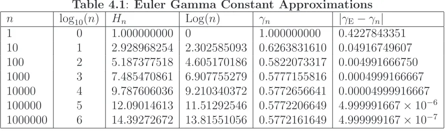
[image:25.612.91.539.95.226.2]the closed-form given by equation (4.31). A summary of computations of the approximations of the constant over increasing inputsn is given in Table 4.1.
Table 4.1: Euler Gamma Constant Approximations
n log10(n) Hn Log(n) γn |γE−γn|
1 0 1.000000000 0 1.000000000 0.4227843351 10 1 2.928968254 2.302585093 0.6263831610 0.04916749607 100 2 5.187377518 4.605170186 0.5822073317 0.004991666750 1000 3 7.485470861 6.907755279 0.5777155816 0.0004999166667 10000 4 9.787606036 9.210340372 0.5772656641 0.00004999916667 100000 5 12.09014613 11.51292546 0.5772206649 4.999991667×10⁻⁶
1000000 6 14.39272672 13.81551056 0.5772161649 4.999999167×10⁻⁷
5
The
j
-Factorial Polynomials
5.1
Motivation and Background
The definition of the Stirling convolution polynomial sequence, denoted by σn(x), and corresponding enumerations suggest a generalization that results in an extended set of parametrized α-factorial polynomial sequences, denoted by σα
n(x) [24, §6; cf. (7.52)] [32]
[3, cf. §4] [50, cf. §4.8]. Additional polynomials related to the classical Stirling number tri-angles considered in the referenced literature include the C-numbers [16, (3.14)] and other combinatorial-based polynomial forms defined by the contexts of individual applications [11,
§12] [22; 61].
The approach to defining the generalized polynomials is based on treating the triangle entries in equations (3.1) and (3.2) as polynomials in the upper coefficient index, as is used to define the polynomials corresponding to the existing expansions of the classical Stirling triangles. The polynomials corresponding to the Stirling numbers of the first kind are formed by the variant Newton series expansion identity in terms of the “second-order” Eulerian number triangle given by the next equation [A008517] [24, (6.44) and (6.45); cf. (6.43)] [32, cf. “Asymptotics”].
x x−n
=
n
X
k=0
n k
x+k
2n
It happens that considering the coefficient expansions with the known factors in the sum removed from the expansion of each binomial term results in forms that are particularly revealing with respect to the underlying structure of each triangle expressed by the generating function enumerating the polynomials. The Stirling (convolution) polynomial sequence is defined by the enumeration of equation (5.1) [24, §6.2].
∞
X
n=0
xσn(x)zn :=
∞
X
n=0
x x−n
(x−n−1)! (x−1)! z
n =
zez ez −1
x
The given generating function for the Stirling polynomial sequence satisfies the requirements of the more general form ofconvolution polynomial sequences [32] and so may be expressed in terms of the characteristic identities of these forms, including the table of convolution prop-erties provided in the primary reference on the sequence [24, Table 272 and§6.5]. Additional properties of the sequence of Stirling polynomials in relation to the generalized α-factorial polynomial sequences are considered in §5.3.5.
5.2
j
-Factorial Polynomial Definitions and Generating Functions
5.2.1 Generalized Polynomials of the First Kind
The α


![Table 6.1:x1(s! ( − Full-Indexed Quadruple-Factorial Expansions−1)x+1 [zx]S�(x; z) 1)](https://thumb-ap.123doks.com/thumbv2/123dok/937202.905720/39.612.78.553.429.508/table-full-indexed-quadruple-factorial-expansions-zx-s.webp)