Chapter 5: Modeling and Analysis
Major component
the model base and its
management
Caution
–
Familiarity with major ideas
–
Basic concepts and definitions
–
Tool--the influence diagram
–
Modeling directly in
spreadsheets
Structure of some successful models
and methodologies
–
decision analysis
–
decision trees
–
optimization
–
heuristic programming
–
simulation
New developments in modeling tools
and techniques
Important issues in model base
management.
5.1 Opening Vignette:
Siemens Solar Industries
Saves Millions by Simulation
Clean room contamination-control
technology
No experience
Use simulation: a virtual laboratory
Major benefit: knowledge and insight
Improved the manufacturing process
Saved SSI over $75 million each year
5.2 Modeling for MSS
Modeling
Key element in most DSS
A
necessity
in a model-based DSS
Frazee Paint Company (Appendix A
Three model types
1. Statistical model (regression analysis)
2. Financial model
3. Optimization model
Several models
Standard
Custom made
Major Modeling Issues
Problem identification
Environmental analysis
Variable identification
Forecasting
Multiple model use
Model categories (or selection)
[Table 5.1]
Model management
Knowledge-based modeling
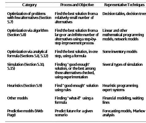
TABLE 5.1 Categories of Models.
Category
Process and Objective
Representative Techniques
Optimization of problems
with few alternatives (Section
5.7)
Find the best solution from a
relatively small number of
alternatives
Decision tables, decision trees
Optimization via algorithm
(Section 5.8)
Find the best solution from a
large or an infinite number of
alternatives using a
step-by-step improvement process
Linear and other
mathematical programming
models, network models
Optimization via analytical
formula (Sections 5.8, 5.12)
Find the best solution, in one
step, using a formula
Some inventory models
Simulation (Section 5.10,
5.15)
Finding "good enough"
solution, or the best among
those alternatives checked,
using experimentation
Several types of simulation
Heuristics (Section 5.9)
Find "good enough" solution
using rules
Heuristic programming,
expert systems
Other models
Finding "what-if" using a
formula
Financial modeling, waiting
lines
Predictive models (Web
Page)
Predict future for a given
scenario
Forecasting models, Markov
analysis
5.3 Static and Dynamic Models
Static Analysis
–
Single snapshot
Dynamic Analysis
–
Dynamic models
–
Evaluate scenarios that change over
time
–
Are
time dependent
–
Show
trends
and patterns over time
–
Extended static models
5.4 Treating Certainty,
Uncertainty, and Risk
Certainty Models
Uncertainty
Risk
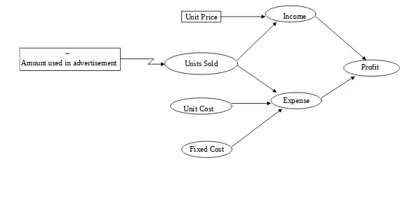
5.5 Influence Diagrams
Graphical representations of a model to assist in
model design, development and understanding
Provide visual communication to the model
builder or development team
Serve as a framework for expressing the MSS
model relationships
Rectangle = a decision variable
Circle = uncontrollable or intermediate
variable
Oval = result (outcome) variable:
intermediate or final
Variables connected with arrows
Example in Figure 5.1
FIGURE 5.1 An Influence Diagram for the Profit Model.
~
Amount used in advertisement Profit Income
Expense Unit Price
Units Sold
Unit Cost
Fixed Cost
5.6 MSS Modeling in
Spreadsheets
(Electronic) spreadsheet: most
popular
end-user modeling tool
Powerful financial, statistical,
mathematical, logical, date/time,
string functions
External add-in functions and solvers
Important for analysis, planning,
modeling
Programmability (macros)
What-if analysis
Goal seeking
Seamless integration
Microsoft Excel
Lotus 1-2-3
Figure 5.2: Simple loan
calculation model (static)
Figure 5.3: Dynamic
5.7 Decision Analysis
of Few Alternatives
(Decision Tables and Trees)
Single Goal Situations
–
Decision tables
–
Decision trees
Decision Tables
Investment Example
One goal: Maximize the yield
after one year
Yield depends on the status of
the economy
(the
state of nature
)
–
Solid growth
–
Stagnation
–
Inflation
1. If there is solid growth in the
economy, bonds will yield 12 percent;
stocks, 15 percent; and time deposits,
6.5 percent
2. If stagnation prevails, bonds will
yield 6 percent; stocks, 3 percent; and
time deposits, 6.5 percent
3. If inflation prevails, bonds will yield 3
percent; stocks will bring a loss of 2
percent; and time deposits will yield
6.5 percent
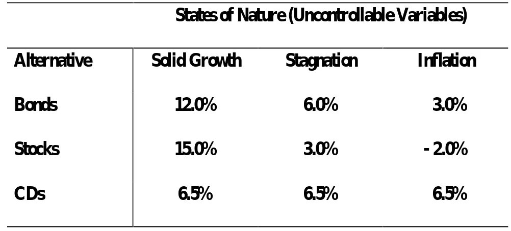
View problem as a
two-person game
Payoff Table 5.2
–
Decision variables (the
alternatives)
–
Uncontrollable variables (the
states of the economy)
–
Result variables (the projected
yield)
TABLE 5.2 Investment Problem Decision Table Model.
States of Nature (Uncontrollable Variables)
Alternative
Solid Growth
Stagnation
Inflation
Bonds
12.0%
6.0%
3.0%
Stocks
15.0%
3.0%
- 2.0%
CDs
6.5%
6.5%
6.5%
Treating Uncertainty
Optimistic approach
Pessimistic approach
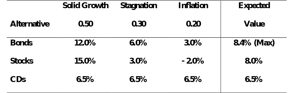
Treating Risk
Use known probabilities
(Table 5.3)
Risk analysis: Compute
expected values
Can be dangerous
TABLE 5.3 Decision Under Risk and Its Solution.
Alternative
Solid Growth
0.50
Stagnation
0.30
Inflation
0.20
Expected
Value
Bonds
12.0%
6.0%
3.0%
8.4% (Max)
Stocks
15.0%
3.0%
- 2.0%
8.0%
CDs
6.5%
6.5%
6.5%
6.5%
Decision Trees
Other Methods of Treating Risk
–
Simulation
–
Certainty factors
–
Fuzzy logic.
Multiple Goals
Table 5.4: Yield, safety, and
liquidity
TABLE 5.4 Multiple Goals.
Alternatives
Yield
Safety
Liquidity
Bonds
8.4%
High
High
Stocks
8.0%
Low
High
CDs
6.5%
Very High
High
TABLE 5.5 Discrete versus Continuous
Probability Distributions.
Discrete
Continuous
Daily Demand
Probability
5
0.10
Normally
6
0.15
distributed with
7
0.30
a mean of
8
0.25
7 and a standard
9
0.20
deviation of 1.2
Decision Support Systems and Intelligent Systems, Efraim Turban and Jay E. Aronson Copyright 1998, Prentice Hall, Upper Saddle River, NJ
5.8 Optimization via
Mathematical Programming
Linear programming (LP) used
extensively in DSS
Mathematical Programming
Family of tools to solve managerial
problems in allocating scarce
resources among various activities
to optimize a measurable goal
LP Allocation
Problem Characteristics
1.Limited quantity of economic
resources
2.Resources are used in the
production of products or services.
3.Two or more ways (solutions,
programs) to use the resources
4.Each activity (product or service)
yields a return in terms of the goal
5.Allocation is usually restricted by
constraints
LP Allocation Model
Rational Economic Assumptions
1. Returns from different allocations can be
compared in a common unit
2. Independent returns
3. Total return is the sum of different
activities’ returns
4. All data are known with certainty
5. The resources are to be used in the most
economical manner
Optimal solution: the best, found
algorithmically
Linear Programming
Decision variables
Objective function
Objective function
coefficients
Constraints
Capacities
Input-output (technology)
coefficients
5.9 Heuristic Programming
Cuts the search
Gets
satisfactory
solutions more
quickly and less expensively
Finds rules to solve complex problems
Heuristic programming finds feasible
and "good enough" solutions to some
complex problems
Heuristics can be
–
Quantitative
–
Qualitative (in ES)
When to Use
Heuristics
1. Inexact or limited input data
2. Complex reality
3. Reliable, exact algorithm not available
4. Simulation computation time too
excessive
5. To improve the efficiency of
optimization
6. To solve complex problems
7. For symbolic processing
8. For solving when quick decisions are
to be made
Advantages of
Heuristics
1. Simple to understand: easier to implement and
explain
2. Help train people to be creative
3. Save formulation time
4. Save programming and storage requirements on
the computers
5. Save computer running time (speed)
6. Frequently produce multiple acceptable solutions
7. Usually possible to develop a measure of solution
quality
8. Can incorporate intelligent search
9. Can solve very complex models
Limitations of Heuristics
1. Cannot guarantee an optimal solution
2. There may be too many exceptions
3. Sequential decision choices can fail
to anticipate future consequences of
each choice
4. Interdependencies of subsystems can
influence the whole system
Heuristics successfully applied to
vehicle routing
5.10 Simulation
A
technique for conducting experiments
with a computer on a model of a
management system
Frequently used DSS tool
Major Characteristics of Simulation
–
Simulation
imitates
reality and capture its
richness
–
Simulation is a technique for
conducting
experiments
–
Simulation is a
descriptive
not normative tool
–
Simulation is often used to solve very
complex, risky problems
Advantages of
Simulation
1. Theory is straightforward
2.
Time compression
3. Descriptive, not normative
4. Intimate knowledge of the problem
forces the MSS builder to interface with
the manager
5. The model is built from the manager's
perspective
6. No generalized understanding is required
of the manager. Each model component
represents a real problem component
7. Wide variation in problem types
8. Can experiment with different variables
9. Allows for real-life problem
complexities
10. Easy to obtain many performance
measures directly
11. Frequently the only DSS modeling tool
for handling nonstructured problems
12. Monte Carlo add-in spreadsheet
packages (@Risk)
Limitations of
Simulation
1. Cannot guarantee an optimal
solution
2. Slow and costly construction
process
3. Cannot transfer solutions and
inferences to solve other problems
4. So easy to sell to managers, may
miss analytical solutions
5. Software is not so user friendly
Simulation
Methodology
Set up a model of a real system
and conduct repetitive
experiments
1. Problem Definition
2. Construction of the Simulation Model
3. Testing and Validating the Model
4. Design of the Experiments
5. Conducting the Experiments
6. Evaluating the Results
7. Implementation
Simulation Types
Probabilistic Simulation
–
Discrete distributions
–
Continuous distributions
–
Probabilistic simulation via Monte
Carlo technique
–
Time Dependent versus Time
Independent Simulation
–
Simulation Software
–
Visual Simulation
–
Object-oriented Simulation
5.11 Multidimensional Modeling
From a spreadsheet and analysis
perspective
2-D to 3-D to multiple-D
Multidimensional modeling tools:
16-D +
Multidimensional modeling: four
views of the same data (Figure 5.5)
Tool can compare, rotate, and "slice
and dice" corporate data across
different management viewpoints
5.12 Visual Spreadsheets
User can visualize the
models and formulas using
influence diagrams
Not cells, but symbolic
elements (Figure 5.6)
English-like modeling
5.13 Financial and Planning
Modeling
Special tools to build usable
DSS rapidly, effectively, and
efficiently
The models are
algebraically
oriented
Definition and
Background of Planning
Modeling
Fourth generation programming
languages
Models written in an English-like
syntax
Models are self-documenting
Model steps are nonprocedural
Examples
–
Visual IFPS / Plus
–
ENCORE Plus!
–
SORITEC
–
Some are embedded in EIS and OLAP tools
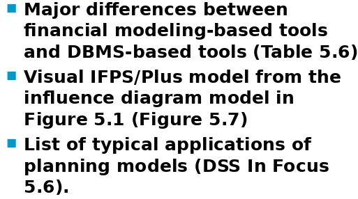
Major differences between
financial modeling-based tools
and DBMS-based tools (Table 5.6)
Visual IFPS/Plus model from the
influence diagram model in
Figure 5.1 (Figure 5.7)
List of typical applications of
planning models (DSS In Focus
5.6).
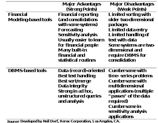
[image:42.720.171.684.79.365.2]TABLE 5.6 Comparison of Financial Modeling Generators
with Those Based Around DBMS.
Major Advantages
(Strong Points)
Major Disadvantages
(Weak Points)
Financial
Modeling-based tools
Financial reporting
(and consolidations
with some systems)
Forecasting
Sensitivity analysis
Usually easier to learn
for financial people
Many built-in
financial and
statistical routines
Limited sorting with
older two-dimensional
packages
Limited data entry
Limited handling of
text with data
Some systems are
two-dimensional and
require DBMS for
consolidation
DBMS-based tools
Data (record)-oriented
Best text handling
Best sort/merge
Data integrity
Strong in ad hoc,
unstructured queries
and analysis
Cumbersome with
time- series problems
Cumbersome with
multidimensional
applications (multiple
"passes" of the data
required)
Cumbersome in
sensitivity analysis
applications
Source: Developed by Neil Dorf, Xerox Corporation, Los Angeles, CA.
COLUMNS 2000..2010
\Model to show relationships among variables \
\ Annual Result Variable:
PROFIT = INCOME - EXPENSE \
\ Decision Variable:
AMOUNT USED IN ADVERTISEMENT = 10000, PREVIOUS * 1.1 \
\ Intermediate Result Variables:
INCOME = UNITS SOLD * UNIT PRICE
EXPENSE = UNITS COST * UNIT PRICE + FIXED COST
\
UNITS SOLD = .5 * AMOUNT USED IN ADVERTISEMENT \
\ Initial Data:
UNIT COST = 10, PREVIOUS * 1.05 UNIT PRICE = 20, PREVIOUS * 1.07
FIXED COST = 50000, PREVIOUS * .5, PREVIOUS * .9 \
\ To Complete the Model, we normally would take a Net Present Value Calculation:
DISCOUNT RATE = 8%
NET PRESENT VALUE PROFIT = NPVC(INCOME, DISCOUNT RATE, EXPENSE)
FIGURE 5.7 IFPS Model and Solution of the Profit Model
Shown in the Influence Diagram in Figure 5.1. The model has been expanded
to include expressions for the unknown initial data and for the decision
variable.
D
S
S
In
Fo
cu
s
5
.6
: Typ
ica
l Ap
p
lica
tio
n
s
o
f P
la
n
n
in
g
M
o
d
e
ls
Fin
a
n
cia
l fo
re
ca
s
tin
g
M
a
n
p
o
w
e
r p
la
n
n
in
g
P
ro
fo
rm
a
fi
n
a
n
cia
l s
ta
te
m
e
n
ts
P
ro
fi
t p
la
n
n
in
g
Ca
p
ita
l b
u
d
g
e
tin
g
S
a
le
s
fo
re
ca
s
tin
g
M
a
rke
t d
e
cis
io
n
m
a
kin
g
In
ve
s
tm
e
n
t a
n
a
lys
is
M
e
rg
e
rs
a
n
d
a
cq
u
is
itio
n
s
a
n
a
lys
is Co
n
s
tru
ctio
n
S
ch
e
d
u
lin
g
Le
a
s
e
ve
rs
u
s
p
u
rch
a
s
e
d
e
cis
io
n
s
Ta
x P
la
n
n
in
g
P
ro
d
u
ctio
n
s
ch
e
d
u
lin
g
En
e
rg
y re
q
u
ire
m
e
n
ts
N
e
w
ve
n
tu
re
e
va
lu
a
tio
n
La
b
o
r co
n
tra
ct n
e
g
o
tia
tio
n
fe
e
s
Fo
re
ig
n
cu
rre
n
cy a
n
a
lys
is
5.14 Visual Modeling and
Simulation
Visual interactive modeling (VIM) (DSS In
Action 5.8)
Also called:
–
Visual interactive problem solving
–
Visual interactive modeling
–
Visual interactive simulation
Use computer graphics to present the
impact of different management decisions.
Users perform sensitivity analysis
Static or a dynamic (animation) systems
(Example: Figure 5.8)
Visual Interactive
Simulation (VIS)
Decision makers interact
with the simulated model
and watch the results over
time
Visual Interactive Models
and DSS
–
VIM (Case Application W5.1 on
the Book’s Web Site)
–
Queuing
5.15 Ready-made Quantitative
Software Packages
Preprogrammed models can expedite
the programming time of the DSS
builder
Some models are building blocks of
other quantitative models
–
Statistical Packages
–
Management Science Packages
–
Financial Modeling
–
Other Ready-Made Specific DSS
(Applications)
–
including spreadsheet add-ins
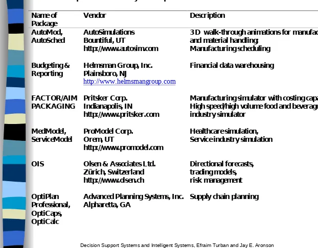
TABLE 5.7 Representative Ready-made Specific DSS
Name of
Package
Vendor
Description
AutoMod,
AutoSched
AutoSimulations
Bountiful, UT
http://www.autosim.com
3 D walk-through animations for manufacturing
and material handling;
Manufacturing scheduling
Budgeting &
Reporting
Helmsman Group, Inc.
Plainsboro, NJ
http://www.helmsmangroup.com
Financial data warehousing
FACTOR/AIM
PACKAGING
Pritsker Corp.
Indianapolis, IN
http://www.pritsker.com
Manufacturing simulator with costing capabilities,
High speed/high volume food and beverage
industry simulator
MedModel,
ServiceModel
ProModel Corp.
Orem, UT
http://www.promodel.com
Healthcare simulation,
Service industry simulation
OIS
Olsen & Associates Ltd.
Zürich, Switzerland
http://www.olsen.ch
Directional forecasts,
trading models,
risk management
OptiPlan
Professional,
OptiCaps,
OptiCalc
Advanced Planning Systems, Inc.
Alpharetta, GA
Supply chain planning
PLANNING
WORKBENCH
Proasis Ltd.
Chislehurst, Kent, England
http://www.proasis.co.uk
Graphically-based planning system
for the process industry
StatPac Gold
Stat Pac Inc.
Edina, MN
Survey analysis package
TRAPEZE
Trapeze Software Group
Mississauga, ON
http://www.trapsoft.com
Planning, scheduling and
operations
TruckStops,
OptiSite,
BUSTOPS
MicroAnalytics, Inc.
Arlington, VA
Distribution management and
transportation
5.16 Model Base Management
MBMS: capabilities similar to that
of DBMS
But, there are no comprehensive
model base management
packages
Each organization uses models
somewhat differently
There are many model classes
Some MBMS capabilities require
expertise and reasoning
Desirable Capabilities of
MBMS
Control
Flexibility
Feedback
Interface
Redundancy Reduction
Increased Consistency
MBMS Design Must
Allow the DSS User to
1. Access and retrieve existing
models.
2. Exercise and manipulate
existing models
3. Store existing models
4. Maintain existing models
5. Construct new models with
reasonable effort
Modeling Languages
Relational MBMS
Object-oriented Model Base and Its
Management
Models for Database and MIS
Design and their Management
Enterprise and Business Process
Reengineering Modeling and Model
Management Systems
SUMMARY
Models play a major role in DSS
Models can be static or dynamic.
Analysis is under assumed certainty,
risk, or uncertainty
–
Influence diagrams
–
Electronic spreadsheets
–
Decision tables and decision trees
Optimization tool: mathematical
programming
Linear programming:
economic-base
Heuristic programming
Simulation
Simulation can deal with more
complex situations
Expert Choice
Forecasting methods
Multidimensional modeling
Decision Support Systems and Intelligent Systems, Efraim Turban and Jay E. Aronson Copyright 1998, Prentice Hall, Upper Saddle River, NJ
Built-in quantitative models (financial,
statistical)
Special financial modeling languages
Visual interactive modeling
Visual interactive simulation (VIS)
Spreadsheet modeling and results in
influence diagrams
MBMS are like DBMS
AI techniques in MBMS
Decision Support Systems and Intelligent Systems, Efraim Turban and Jay E. Aronson Copyright 1998, Prentice Hall, Upper Saddle River, NJ
Questions for the Opening
Vignette
1.
Explain how simulation was used to evaluate a
nonexistent system.
2.
What was learned, from using the simulation
model, about running the clean room?
3.
How could the time compression capability of
simulation help in this situation?
4.
How did the simulation results help the SSI
engineers learn about their decision making
problem? Were they able to focus better on
the structure of the real system? How did this
save development and operating costs of the
real clean room?
Debate
Some people believe that
managers do not need to know
the internal structure of the
model and the technical aspects
of modeling. “It is like the
telephone or the elevator, you
just use it.” Others claim that this
is not the case and the opposite
is true. Debate the issue.
Class Exercises
3. Everyone in the class Write your
weight, height and gender on a piece of
paper (no names please!).
Create a regression (causal) model for
height versus weight for the whole class,
and one for each gender.
If possible, use a statistical package and
a spreadsheet and compare their ease of
use.
Produce a scatterplot of the three sets of
data.
Do the relationships appear linear?
How accurate were the models (R
2
)?
Does weight
cause
height; does
height
cause
weight; or does neither
really
cause
the other? Explain?
How can a regression model like this
be used in building design; diet /
nutrition selection? in a longitudinal
study (say over 50 years) in
determining whether students are
getting heavier and not taller, or
vice-versa?
6. DSS generators are English-like and have a variety of analysis
capabilities.
–
a. Identify the purpose and the analysis capabilities of the following IFPS
program:
MODEL FIRST
COLUMNS 1-5INVESTMENT = LAND + BUILDING RETURN = SALES - COSTS
PRESENT VALUE = NPVC(RETURN, DISCOUNT RATE, INVESTMENT) INTERNAL RATE OF RETURN = IRR(RETURN, INVESTMENT)
\ INPUT DATA LAND = 200, 0
BUILDING = 100, 150, 0
SALES = 500, PREVIOUS + 100
COSTS = SUM(MATERIALS THRU LABOR) MATERIALS = 10 + 0.20 * SALES
OVERHEAD = .10 * SALES LABOR = 20 + 0.40 * SALES
DISCOUNT RATE = 0.20, PREVIOUS
b. Change sales to be under assumed risk, that
is, replace the SALES line and insert a line
following it:
–
9 SALES = NORRANDR(EXPECTED SALES, EXPECTED
SALES/10)
–
EXPECTED SALES = 500, PREVIOUS + 100
and use
–
MONTE CARLO 200
–
COLUMNS 5
–
HIST PRESENT VALUE, INTERNAL RATE OF RETURN
–
FREQ PRESENT VALUE, INTERNAL RATE OF RETURN
–
NONE
What do these statements do to this new model?
12.Use the Expert Choice software to
select your next car. Evaluate cars on ride
(from poor to great), looks (from
attractive to ugly), and acceleration
(seconds per first 50 yards).
–
Consider three final cars on your list. Develop:
–
a. Problem hierarchy
–
b. Comparison of the importance of the criteria
against the goal
–
c. Comparison of the alternative cars for each
criterion
–
d. An overall ranking (synthesis of leaf nodes
with respect to goal)
e. A sensitivity analysis.
Maintain the inconsistency index lower than 0.1. If
you initially had an inconsistency index greater
than 0.1, what caused it to be that high? Would you
really buy the car you selected? Why or why not?
Also develop a spreadsheet model using estimated
weights and estimates for the intangible items,
each on a scale from 1-10 for each car.
Compare the conclusions reached with this method
to those found in using the Expert Choice Model.
Which one more accurately captures your
judgments and why?
14. Job Selection Using Expert
Choice. You are on the job market
(use your imagination, if
necessary). List the names of four
or five different companies that
have offered you a job (or from
which you expect to get an offer).
(As an alternative, your instructor
may assign Graduate or
Undergraduate Program Selection.)
Write down all the factors that may
influence your decision as to which job
offer you will accept. Such factors may
include but need not be limited to
geographic location, salary, benefits,
taxes, school system (if you have
children), and potential for career
advancement. Some of these factors
(criteria, attributes) may have
sub-criteria. For instance, location may be
sub-divided further into climate, urban
concentration, cost of living, etc.
If you, in fact, do not yet have
a dollar salary figure
associated with a job offer,
you should just guess a
"reasonable" figure. Perhaps
your classmates can help you
in determining realistic
figures.
a. Model this problem in a spreadsheet
(Excel) using some kind of
Weighted
Average Methodology
[you set the
criteria weights first] (see the current
Rand-McNally
Places Rated Almanac
for
an example).
b. Construct an Expert Choice model for
your decision problem, and use the
pairwise comparisons to arrive at the
"best" job opportunity.
c. Compare the two approaches. Did they
yield the same results? Why or why not?
d. Write a short report (one or two typed pages)
explaining the results including those of the
Weighted Average Methodology, and for Expert
Choice: each criterion, sub-criterion (if any) and
alternative. Describe (briefly) which options and
capabilities of Expert Choice you used in your
analysis, and show the numerical results of your
analysis. To this purpose, you may want to include
printouts of your AHP tree, but make sure you circle
and explain the parts of interest on these printouts.
Discuss the nature of the tradeoffs you encountered
during the evaluation process. You may want to
include a (meaningful) sensitivity analysis of the
results, but this is optional (for this assignment).
To think about:
Was the
Expert Choice analysis helpful
in structuring your
preferences? Do you think it
will be a helpful aid in your
actual decision making
process? Comment on all
these issues in your report.
Term Paper
Select a current DSS technology or
methodology. Write up a 5 page
report detailing the origins of the
technology, what need prompted the
development of the technology, and
what the future holds for it over the
next 2, 5 and 10 years. Use electronic
sources, if possible, to identify
companies providing the technology.
If demo software is available, acquire
it and include a sample run in your
paper